Location Allocation of Sugar Beet Piling Centers Using GIS and Optimization - MDPI
←
→
Page content transcription
If your browser does not render page correctly, please read the page content below
infrastructures
Article
Location Allocation of Sugar Beet Piling Centers
Using GIS and Optimization †
Nimish Dharmadhikari 1, *              and Kambiz Farahmand 2
 1    Transportation Modeling Coordinator, 2 West Second Street, Suite 800, Tulsa, OK 74103, USA
 2    Industrial and Manufacturing Engineering, North Dakota State University, Department 2485, PO Box 6050,
      Fargo, ND 58108-6050, USA; Kambiz.Farahmand@ndsu.edu
 *    Correspondence: ndharmadhikari@incog.org; Tel.: +1-918-579-9423
 †    This paper won the Best Student Paper award at the 2019 AASHTO GIS-T Symposium in Kissimmee, FL,
      USA. It has been modified for publishing in the journal.

 Received: 8 March 2019; Accepted: 17 April 2019; Published: 23 April 2019

 Abstract: The sugar beet is one of the most important crops for both social and economic reasons,
 even though the area under sugar beet cultivation in the Red River valley of North Dakota and
 Minnesota is comparatively smaller that of corn and other crop lands. It generates a large
 economic activity in local and regional level with a greater impact on jobs and stimulation of
 agriculture, transportation, and farm economy. Sugar beet transportation takes place in two stages in
 Red River Valley: the first step is from farms to piling centers (pilers) and the second step from pilers
 to processing facilities. This study focuses on the problem of optimizing piler locations based on
 supply variation. Sugar beet supply and harvest varies significantly due to numerous reasons such as
 weather, water availability, and different maturity dates for the crop. This provides for a variable
 optimal harvesting time based on the plant maturity and sugar content. Sub-optimized pilers location
 result in the high transportation and utilization costs. The objective of this study is to minimize the
 sum of transportation costs to and from pilers and the pilers utilization cost. A two-step algorithm
 based on the geographical information system (GIS) with global optimization method is used to solve
 this problem. This method will also be useful for infrastructure decision makers such as planners and
 engineers to predict the truck volume on rural roads.

 Keywords: optimization; GIS; location; sugar beet; infrastructure decision making

1. Introduction
      The sugar beet is considered as one of the most important crops in Red River Valley of North Dakota
and Minnesota in the United States. According to Farahmand et al. [1] this sugar beet co-op operation
is the largest sugar beet producer in the United States. The co-op is owned by about 2800 shareholders
who raise nearly 40% of the nation’s sugar beet acreage. They also mentioned that the last seeding
usually takes place on June 20 while full stockpile harvest starts on October 1st. This explains the
seasonal nature of sugar beet harvesting. American Crystal Sugar Company (ACSC) manages this
co-op. ACSC has five processing facilities in the Red River Valley as shown in Figure 1.
      Growers are responsible for delivering the crop to the piling centers. ACSC operates the piling
centers for growers to deliver the load to five processing factories. Beets get unloaded at the piling
center (piler) in piles and the responsibility shifts from grower to the ACSC. At the pilers, sugar beets
are cleaned and are piled 300 tall x 2400 long for long term storage through the winter. The beets need
to stay cold and frozen for long term storage or otherwise they will rot. At processing time, these beets
are loaded on the truck using conveyors. Once the truck is full, a new truck takes over loading the

Infrastructures 2019, 4, 17; doi:10.3390/infrastructures4020017              www.mdpi.com/journal/infrastructures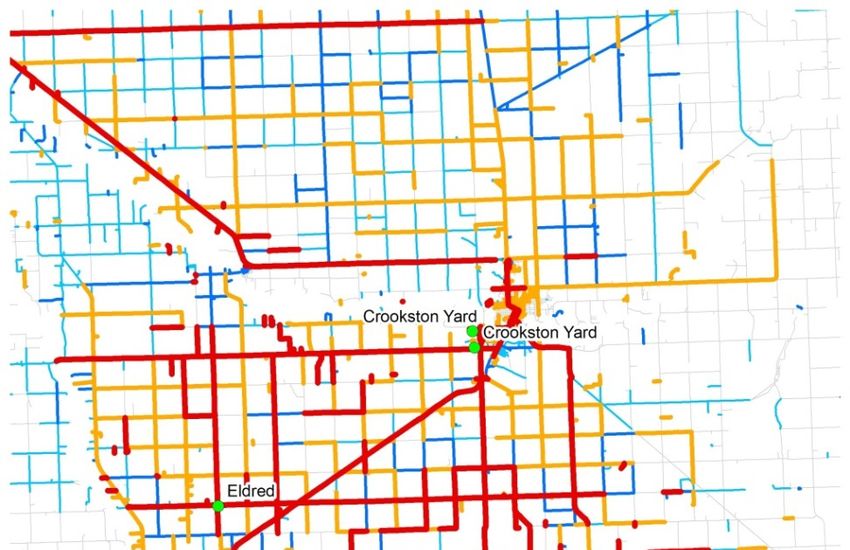
Infrastructures 2019, 4, 17 2 of 15
Infrastructures
beets. 2018, 3, trucks
The loaded x FOR PEER REVIEW
drive 2 of 15
to the nearest sugar beet processing plant or receiving station. Figure 2
depicts this logistics system of sugar beet transportation from farms to processing plants.
Figure 1. Sugar beet region and processing facilities in North Dakota and Minnesota.
Growers are responsible for delivering the crop to the piling centers. ACSC operates the piling
centers for growers to deliver the load to five processing factories. Beets get unloaded at the piling
center (piler) in piles and the responsibility shifts from grower to the ACSC. At the pilers, sugar beets
are cleaned and are piled 30′ tall x 240′ long for long term storage through the winter. The beets need
to stay cold and frozen for long term storage or otherwise they will rot. At processing time, these
beets are loaded on the truck using conveyors. Once the truck is full, a new truck takes over loading
the beets. The loaded trucks drive to the nearest sugar beet processing plant or receiving station.
Figure 2 Figure
depicts1.
Figure 1.this
Sugar
Sugar logistics
beet system
beet region
region andof
and sugar beet
processing
processing transportation
facilities
facilities in
in North from and
North Dakota
Dakota farms to processing plants.
and Minnesota.
Minnesota.
Some beets are directly transported to the processing plants without storing them. This process
isSome
Growersbeets
dependent areare
on directly
differenttransported
responsible factors. to thethe
Farmers
for delivering processing
and ACSC
crop to theplants
decide
pilingwithout
whether
centers.storing
to them.
store
ACSC beetsThis
operates process
or the
to take
pilingis
them
dependent
centers for on
to processing different
growersplant factors.the
directly.
to deliver Farmers
This toand
decision
load fiveACSC decide
isprocessing
mainly based whether tomaturity
on theBeets
factories. store
getbeets or to
of the
unloaded take
beets. them
The
at the to
mature
piling
processing
center plant
beet(piler)
has the directly.
highest
in piles This
andsugar decision is mainly
content. The shifts
the responsibility paymentbased on
fromreceived the
grower to maturity
bythe of
theACSC. the beets.
farmerAtisthe
basedThe mature
on sugar
pilers, beet
sugarbeets
content
has the highest
are thus
cleaned and sugar
farmers want
are content.
to keep
piled 30′ tall The
the payment
x beets
240′ in the
long received
forground bymaximize
to
long term the farmer
storage is based
sugar
through on sugar
content. ACSC
the winter. content
The desires thus
to start
beets need
farmers want
the harvest
to stay to keep
cold andatfrozen the
an optimal beets
for long in
time the ground
to storage
term ensure theto maximize sugar
processingthey
or otherwise content.
plants
will are ACSC
rot.busy desires
and remain
At processing to start the
at these
time, capacity
harvest
beets at an
throughout optimal
are loadedthe time
onseason.
the truck to ensure
This the
balance
using processing
is important
conveyors. plants
based
Once the are
truck busy
on is and
thefull, remain
planting
a new timeat capacity
truckand
takes throughout
harvesting
over loadingtime in
the season.
order to This balance
minimize cost is important
and maximize based
profit ontothe
the planting
growers. time and
the beets. The loaded trucks drive to the nearest sugar beet processing plant or receiving station. harvesting time in order to
minimize cost and
Figure 2 depicts maximize
this logistics profit
system toof
the growers.
sugar beet transportation from farms to processing plants.
Some beets are directly transported to the processing plants without storing them. This process
is dependent on different factors. Farmers and ACSC decide whether to store beets or to take them
Farm Processing
to processing plant directly. This decision is mainly Pilers based on the maturity of the beets. The mature
beet has the highest sugar content. The payment received by the farmer is based Plant
on sugar content
thus farmers want to keep the beets in the ground to maximize sugar content. ACSC desires to start
the harvest Farm
at an optimal time to ensure the processing plants are busy and remain at capacity
throughout the season. This balance is important based on the planting time and harvesting time in
order to minimize cost and maximize profit to the growers.
Farm
Figure 2. Sugar beet processing.
Farm Processing
Pilers
Figure 2. Sugar beet processing.
Plant
Pilers are considered as natural refrigerators to save beets from rotting. The colder temperatures
PilersValley
in Red River are considered
in winteras natural
helps the refrigerators
beets to staytoatsave beets
pilers for afrom rotting.
longer timeThe
aftercolder temperatures
harvest. Sugar
Farm
beetinroots
Red River Valley
should in winter
be cleaned fromhelps the beets
excessive to stay
dirt, and at pilers
properly for a longer
defoliated time after
and cleaned harvest.
from weed Sugar
or
leaves to allow for proper ventilation while stored in piles. Sugar beets may be stored up to 4 months,
and during this storage period the roots will decay and ferment. As a result, the sugar beet roots
will heat up and the respiration leads to around 70% loss of sucrose. Decay and fermentation during
Farm
storage could also cause sucrose loss of up to 10% and 20%. Some of the sucrose losses caused by the
storage have been reduced through the utilization of forced-air ventilation, cooling in hotter areas and
Figure 2. Sugar beet processing.
Pilers are considered as natural refrigerators to save beets from rotting. The colder temperatures
in Red River Valley in winter helps the beets to stay at pilers for a longer time after harvest. Sugar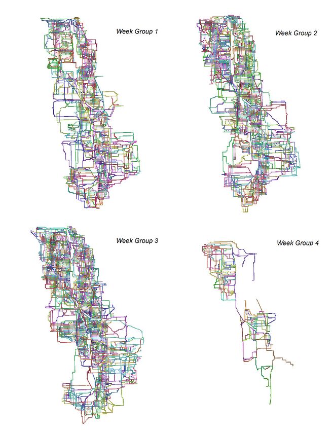
Infrastructures 2019, 4, 17                                                                           3 of 15

subsequent freezing of storage piles after mid-December in colder areas. Ensuring the root temperature
never reaches 55◦ F will keep the roots from decay. During harvest, if air temperature is rising and the
root temperature increases past 55◦ F, the harvest will stop, and no sugar beets will be accepted at the
pilers. This will prevent storage rot. Cold weather and frost could also damage the roots. Foliage and
leaves have proven to provide a natural barrier to frost conditions thus protecting the roots and the
crown area. Exposed roots during a frost shutdown, experience a higher degree of frost damage.
     This situation is ideal for a location allocation problem. The locations of the pilers are to be
optimized to minimize the transportation and storage cost.
     It is really hard for planners and engineers to predict the truck volume on the rural roads.
For infrastructure decisions such as where to add lanes or which road needs widening needs data
for the truck volume. This method will help to predict the truck volume thus it will be an important
method for infrastructure decision makers.
     This article is organized as follows. Section 2 studies the literature available for location allocation
problems in agriculture and other settings. Section 3 describes the methodology and algorithm used
for solution. Section 4 discusses a case study. Section 5 presents sensitivity analysis. Section 6 presents
conclusions along with the path to future research.

2. Literature Review
      Kondor [2] presented the initial problem of the sugar beet transportation. They tried to find the
economic optimum results using the mathematical modeling of the problem. They established the
relation between the processor starting date and the scheduling of the beet arrival. They provide
the case study of Hungary. Scarpari and de Beauclair [3] developed a linear programing model for
sugarcane farm planning. Their model delivered profit maximization and harvest time schedule
optimization. They used GAMS® programing language to solve the problem. They solve this problem
based on the case study of sugarcane farming in Brazil.
      The location problem in a different setting is solved by Esnaf and Küçükdeniz [4]. They presented
the multi-facility location problem (mflp) in logistical network. Their objective is to optimally serve set
of customers by locating facilities. They studied the fuzzy clustering method and developed a hybrid
method. Their method is a two-step method in which the first step uses fuzzy clustering for mflp
and the second step further determines the optimum location using single facility location problem
(sflp). The fuzzy clustering step uses MATLAB® for geographical clustering based on plant customer
assignment. They compared their method with other clustering methods. Costs generated by the
hybrid method are less than other methods. Zhang, Johnson, and Sutherland [5] presented a two-step
method to find the optimum location for biofuel production. Step one uses Geographical Information
System (GIS) to identify feasible facility locations and step two employs total transportation cost model
to select the preferred location. They presented a sensitivity analysis of location study in the Upper
Peninsula of Michigan.
      Houck, Joines, and Kay [6] present the location allocation problem and its solution methodologies.
They examine the applications of genetic algorithm to solve the problem. They propose that these
problems are difficult to solve by traditional optimization techniques thus requiring the use of heuristic
methods. Zhou and Liu [7] propose different stochastic models for the capacitated location allocation
problem. They also propose a hybrid algorithm which integrates network simplex algorithm, stochastic
simulation, and genetic algorithm. They test the effectiveness of this algorithm with numerical
examples. In the further research Zhou and Liu [8] study the location allocation problem with fuzzy
demands. They model this problem in three different minimization models. They propose another
hybrid algorithm to solve these models.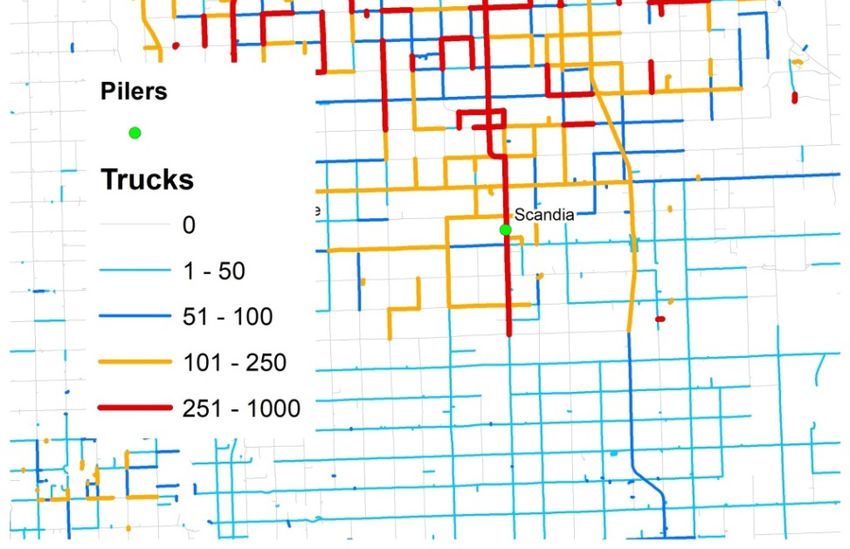
Infrastructures 2019, 4, 17                                                                           4 of 15

       Lucas and Chhajed [9] provided a detailed review of literature in the field of location allocation
involving agricultural problems. They express that there are a lot of location allocation problem
solutions available but there is a lack of application-based research articles. They study six real world
examples. Pathumnakul et al. [10] considered the different maturity times of sugarcane to find the
optimal locations of the loading stations. They modify the fuzzy c-means method to consider cane
maturity time as well as cane supply. Their objective is to minimize the total transportation and
utilization cost. They compare the performance of their method with the traditional fuzzy c-means
method to conclude their method provides a better solution for the problem. They test these methods
with the help of a case study in sugarcane farming in Thailand.
       Another location problem of sugarcane loading stations is studied by Khamjan, Khamjan, and
Pathumnakul [11]. They compare the solution times of the mathematical model and the heuristic
algorithm. Their objective function includes minimization of various costs such as investment cost,
transportation cost, and cost of the sugarcane yield loss. They also applied their model to a case study
to solve the industrial problem. In a recent study Kittilertpaisan and Pathumnakul [12] present a
multiple year crop routing decision problem. Their model includes heuristic algorithm for a three-year
period of sugarcane harvesting. They solve their problem to design the planting and routing such as
sugarcane becomes mature in three years for harvesting.
       Yeh and Chow [13] present an integrated location allocation approach for public facilities planning.
They discuss integration of GIS and location allocation model. They use Hong Kong as an example.
They provide an extensive review of earlier GIS and other location allocation studies. They also provide
an alternating heuristic algorithm.
       Church [14] discusses role of GIS in the location modeling. He presents the history of the use of
GIS in location modeling. He states that GIS provide a richer dataset which can be used to find the
optimal solution of location modeling.
       Murray [15] enlists the contribution of GIS to location science in terms of input data, visualization,
problem solution, and advances in theories. His focus is to showcase the contribution of GIS towards
the advancements of the location allocation modeling theories. He reviews numerous studies showing
the usefulness of GIS in the case of location allocation problem solutions.
       Tolliver et al. [16] present a methodology to estimate the flows from crop zones to elevators and
plants. They also forecast improvement and maintenance costs for roads. They provide a model
with nodes, links, and paths. They provide a simplified grain distribution system. They provide an
exhaustive GIS analysis. They describe the creation of the travel time matrix. They also discuss how
the shortest path between origins and destinations is calculated in GIS using Dijkstra’s algorithm.
       This literature study shows that there are very few articles about sugar production and location
problems and there are nearly zero articles about sugar beet harvesting and location problems involved
in it. The use of GIS is well established for the solution of the location allocation problems as shown in
the literature review. As the numbers of sugar beet fields are large, optimization algorithms suggested
in some of the articles are not applicable in this situation. Also, there are very few articles studying
the seasonal nature of the sugar beet harvest. Based on these problems this article tries to solve the
location allocation problem for sugar beet harvesting using a two-stage GIS based Multi Facility Fuzzy
Clustering (MFFC) algorithm.

3. Methodology
     As stated earlier we use a two-stage method to solve a sugar beet piler location allocation problem.
It involves stage one of GIS analysis with clustering and stage two of optimization. The solution
algorithm is depicted in Figure 3.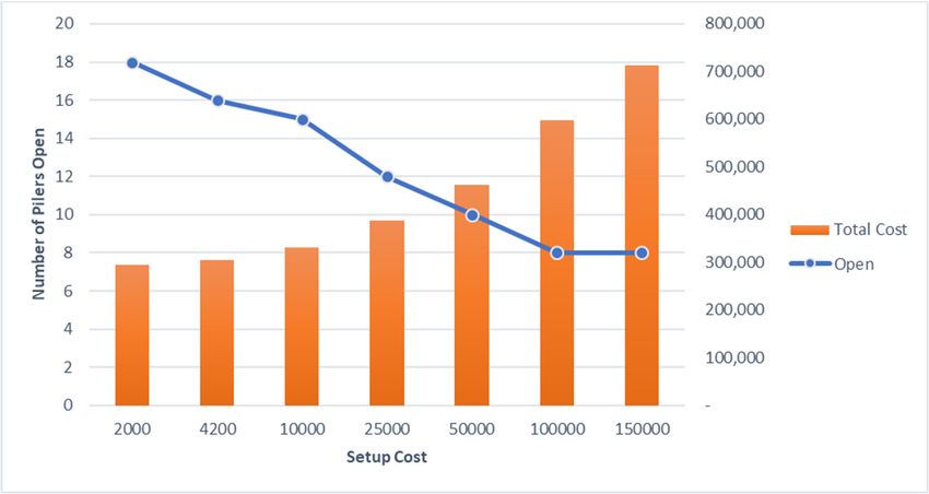
Infrastructures 2018, 3, x FOR PEER REVIEW                                                                   5 of 15
Infrastructures 2019, 4, 17                                                                                  5 of 15

                                              Estimate sugar beet
                                                    Supply

                                             Add weights to farms
                                              based on maturity

                                                                                               Stage 1
                                                     Cluster
                                                     Farms

            Road network                     Add Pilers to clusters

                                                  Generate OD
                                                    matrix

            Weights of
             Farms

          Transportation
                                                  Optimization
               cost                                                                                Stage 2

           Set up and
          operating cost
                                                 Optimized piler
                                                   locations

                              Figure 3. Solution algorithm. O–D: origin–destination.

3.1. Stage 1: GIS Analysis with Clustering
                           Figure 3. Solution algorithm. O–D: origin–destination.

      Stage 1 involves GIS analysis. As stated by Pathumnakul [10] clustering of farms is carried out in
3.1. Stage 1: GIS Analysis with Clustering
this stage. The goal of this stage is to generate an origin–destination (O–D) matrix. A GIS dataset is
      Stage
created      1 involves
          with  different GIS   analysis.
                          shapefiles.  TheAsfarm
                                              stated  by Pathumnakul
                                                   location               [10] clustering
                                                             shapefile is then             of farms
                                                                                added in the        is carried
                                                                                              dataset.         out
                                                                                                       Along with
in
thethis stage.ofThe
     location        goalthis
                 farms,    of this stagealso
                               shapefile  is tohas
                                                generate  an origin–destination
                                                   data about                       (O–D)
                                                               planting dates at each      matrix.
                                                                                        farm,       A GIS
                                                                                               weather     dataset
                                                                                                        conditions,
is
andcreated
      yield. with  different
             Weights          shapefiles.
                       are assigned        The
                                      to the    farm location
                                              locations          shapefile
                                                         of the farms  basedis then added
                                                                               on the       in the
                                                                                      different    dataset.
                                                                                                harvest     Along
                                                                                                         times due
with the location of farms, this shapefile also has data about planting dates at each farm, weather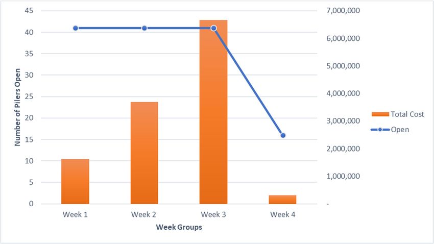
Infrastructures 2019, 4, 17 6 of 15
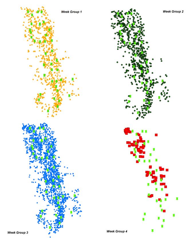
to different planting dates and weather conditions. In this study the weights are expressed in the
preference of the harvest time. This method provides four harvest times: week group 1 is pre-harvest
time which is earlier than peak harvest time, week group 2 and 3 are the peak harvest times, and week
group 4 is post-peak harvest times. To form a complex model these weights in harvest times can be
distributed in more than four groups. The farms are clustered in the groups of four based on these
assigned weights in terms of harvest times. Farms which are planned to be harvested earlier because
of earlier planting dates, weather conditions, or historical preference are clustered in the week group 1,
farms late in the planting date or based on farmers and ACSC’s preference, are clustered in week group
4. These clustered farms are origins. The locations of pilers are also added to this dataset which are
designated as the destinations.
Finally, the road network is added in the dataset. The road network needs to have distances of
each segment in miles, speed limits or observed speed over these segments, and time taken to travel
the distance of each segment (travel time). The GIS software uses a shortest path algorithm to create the
O–D matrix. This method is similar to the method in Dharmadhikari, Lee, and Kayabas [17]. The O–D
matrix can be generated in two ways—1) distance in miles or 2) travel time between O–D pair. For
this process we prefer to use shortest distance in miles which will be used as one of the inputs for
optimization stage.
3.2. Stage 2: Optimization
The aim of the Stage two is to perform the optimization to find the pair of operating pilers
and farms at the given harvest times. This will be a cost optimization process. The objective of the
optimization function is to minimize the cost of logistics. Following are the important inputs for
this process:
1. O–D matrix generated in Stage 1
2. Weights of farms from Stage 1
3. Transportation cost of sugar beets
4. Set up and operating cost of piler
The optimization is performed based on following assumptions:
1. Sum of all shipments should not exceed the total yield at farms
2. Piler is either open or closed at any given time
3. Quantity of sugar beets harvested should not be greater than piler capacity
4. Each sugar beet farm is assigned to one piler only
5. All pilers have the same capacity
The cost of logistics is expressed in terms of addition of different costs involved in the process
such as the cost of transportation, the cost of yield loss if not harvested at the right time, and the cost of
piler operation. These costs are further simplified in terms of the tangible variables which are easy to
measure. These variables are piler set up cost, storage cost, distance, number of trucks, cost per mile
for the truck, and yield loss cost. This gives us Equation (1) for the cost of logistics.
Cost of logistics = (set up cost) + (storage cost) + (distance × number of
(1)
trucks × cost per mile) + (yield loss cost)
The objective function is represented in Equation (2). The objective function states the minimization
of the cost of logistics. It is subject to the sum of all shipments being less than the total yield at
farms (Equation (3)); A Piler can be open or closed (Equation (4)); number of trucks should be greater
than or equal to zero (Equation (5)); yield at the given farm should be greater than or equal to zero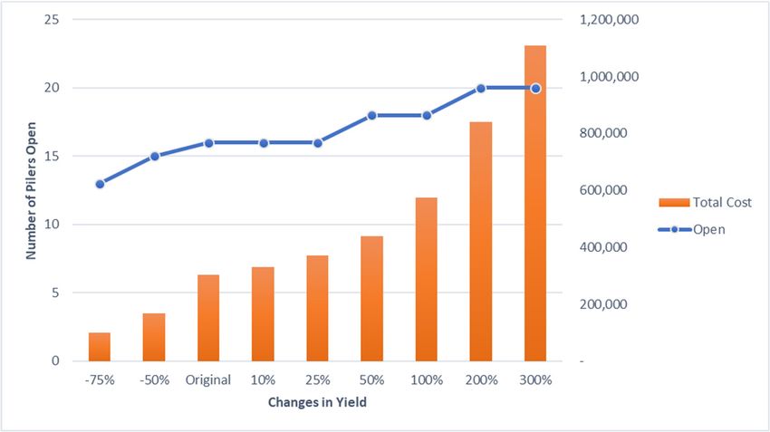
Infrastructures 2019, 4, 17                                                                            7 of 15

(Equation (6)); and quantity of sugar beets harvested should not be greater than total piler capacity
(Equation (7)). The explanation of data sources is presented in the case study section.

                                     n X
                                     X m X
                                         4
           Minimize Cl = Minimize                     Suj × Pj + Stj × Pj + Syi + Xijk × Tij × Cd         (2)
                                      i=1 j=1 k=1

Subject to :
                                          n X
                                          X m
                                                      Tij × Pj × t ≤ Y                                    (3)
                                           i=1 j=1

                                                Pj ∈ {0, 1} ∀ j                                           (4)

                                                    Tij ≥ 0 ∀ i, j                                        (5)

                                                     yi ≥ 0 ∀ i                                           (6)
                                               m
                                               X
                                                      Ij × Pj ≥ Y                                         (7)
                                                j=1

Where,

      Xijk = distance (miles)
      i = number of farms (1, 2, . . . n)
      j = number of pilers (1, 2, . . . m)
      k = number of distance (1, 2, 3, 4)
      yi = yield at farm ‘i’ (tons)
      Y = total yield from all farms = yi
                                         P

      t = sugar beet truck capacity (tons)
      Tij = number of trucks from farm i to piler j = yi/t
      Cd = cost per mile
      Ij = capacity of the piler
      Suj = set up cost of piler j
      Stj = storage cost at piler j
      Syi = yield loss cost at farm i
      Pj = 0 or 1 = Piler is used or not used
      Cl = cost of logistics

4. Case Study
       Red River Valley of North Dakota and Minnesota is the study area. This area involves sugar beet
production in nearly 30 counties as depicted in Figure 1. The sugar beet processing is handled by
American Crystal Sugar Company (ACSC). They have five processing plants at locations Moorhead,
Hillsboro, Crookston, East Grand Forks, and Drayton. As explained earlier, sugar beets are transported
first to the piler locations by farmers for storage until ACSC transports them to one of the five processing
plants. These piler locations are shown in the Figure 4 with the road network.

4.1. Data Sources
     ACSC provided locations of the plants, pilers, and farms. These are the most important locations
for the GIS analysis. ACSC also provided data related to the plant dates, costs, and yields at each
farm. The road network was built upon using TIGER shapefiles from American Census Bureau [18].
Two shapefiles for road networks in North Dakota and Minnesota are downloaded. The road networks
are then combined and cleaned. The boundary between these two states is defined by the Red River.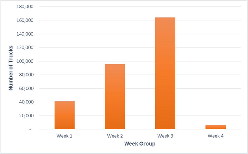
Infrastructures 2019, 4, 17                                                                                       8 of 15

    There are numerous bridges on the river. The cleanup process involved finding locations of the bridges
    and connecting the road network where an existing bridge is present. This helps to provide a combined
    network to use in the GIS analysis. The process followed in this step is similar to the process in
    Dharmadhikari, Lee, and Kayabas [17]. Sugar beet truck fuel efficiency is assumed to be 10 miles per
    gallon and
Infrastructures    average
                2018, 3, x FORfuel
                               PEERcost is assumed to be $3.00 per gallon for the study period.
                                    REVIEW                                                         8 of 15

                                 Figure 4. Red
                                    Figure      River
                                            4. Red    Valley
                                                   River     road
                                                         Valley   network
                                                                road      andand
                                                                     network  piler locations.
                                                                                 piler locations.

4.2.4.2.
     GISGIS Analysis
         Analysis
        Following
     Following   thethe  algorithmshown
                      algorithm        shownin in Figure
                                                  Figure 3,3,GIS
                                                              GISanalysis
                                                                    analysisis is
                                                                               thethe
                                                                                   firstfirst
                                                                                          partpart
                                                                                               of the
                                                                                                    ofstudy.   This analysis
                                                                                                       the study.    This
   involves
analysis     combining
          involves          all dataallsources
                    combining                   and performing
                                         data sources               a clustering
                                                       and performing              model with
                                                                             a clustering     modelthewith
                                                                                                       goal the
                                                                                                              of generating
                                                                                                                  goal of
   origin–destination
generating                (O–D) matrix.
            origin–destination               The road
                                     (O–D) matrix.    Thenetwork     of Red of
                                                            road network      River
                                                                                  RedValley
                                                                                       River is   added
                                                                                                Valley  is in the database.
                                                                                                           added   in the
database. This road network is cleaned and combined as stated in data sources section. Thecontains
   This road  network   is cleaned    and  combined   as stated  in data  sources  section.    The road   network   road
   attributes
network        such attributes
          contains   as name, roadsuch type,   androad
                                         as name,   distance
                                                          type,inand
                                                                  miles   whichinare
                                                                       distance         important
                                                                                     miles           for the
                                                                                              which are        GIS analysis.
                                                                                                          important   for
   Distance  in miles  is  used  in  creation  of the network    dataset.
the GIS analysis. Distance in miles is used in creation of the network dataset.
    Clustering
Clustering
          The sugar beet harvest starts late in months of September and October. Thus, clustering of farms
       The sugar beet harvest starts late in months of September and October. Thus, clustering of farms
    is carried out based on the harvest days. Harvest weeks are divided into four groups. These weeks are
is carried out based on the harvest days. Harvest weeks are divided into four groups. These weeks
    shown in Table 1. The farms are selected based on the harvest days falling within these four categories.
are shown in Table 1. The farms are selected based on the harvest days falling within these four
    Four separate clusters are formed for farms. The selection is carried out using select by attribute tool.
categories. Four separate clusters are formed for farms. The selection is carried out using select by
   These clusters are shown in Figure 5. By visual inspection, week group 2 and week group 3 have
attribute tool. These clusters are shown in Figure 5. By visual inspection, week group 2 and week
    the largest number of farms in the cluster. The locations of the pilers are also added in this database.
group 3 have the largest number of farms in the cluster. The locations of the pilers are also added in
   The small green pins in Figure 5 are the locations of the pilers.
this database. The small green pins in Figure 5 are the locations of the pilers.
                                                  Table 1. Week group division.
                                                Table 1. Week group division.
                              Harvest Weeks
                   Harvest Weeks                                       Days Days
                                                                            of Year
                                                                                  of Year
                   Week Group Week
                              1    Group 1                             Lessorthan
                                                                 Less than        or equal
                                                                               equal to 280 to 280
                   Week Group Week
                              2    Group 2                               281–287281–287
                   Week Group Week
                              3    Group 3                               288–294288–294
                   Week Group Week
                              4    Group 4                                  More294
                                                                      More than    than 294
Infrastructures  2018, 3, 2019,
           Infrastructures x FOR   PEER REVIEW
                                4, 17                                                                                   9 of 15   9 of 15

                                      Figure 5. Sugar beet farm clusters based on Week groups.
                                Figure 5. Sugar beet farm clusters based on Week groups.
          Closest Facility

Closest facility
             As stated in the methodology section, the clustered farms are connected to the pilers using closest
          facility method from ArcGIS® . This method uses the road network prepared in the data sources section.
      As The
           stated
                cost in  the methodology
                     of travelling                 section,
                                    for this analysis         theonclustered
                                                        is based                  farms
                                                                       the distance        arebetween
                                                                                     in miles    connected
                                                                                                         farm to    the pilers
                                                                                                                (incident)  and using
closest facility     method
          piler (facility).  Thisfrom
                                  method  ArcGIS
                                            finds the. closest
                                                    ®   This method        uses
                                                                piler to any farm.the   roadofnetwork
                                                                                    A total     four closestprepared      in the data
                                                                                                              pilers are found
          for  each farm   to generate   origin–destination    cost matrix.  This  gives us four  distances
sources section. The cost of travelling for this analysis is based on the distance in miles between          in  miles for each farm
(incident)farm.
              andThe   closest
                    piler       facility solution
                            (facility).            routes are
                                         This method            shown
                                                            finds   the in  Figurepiler
                                                                         closest    6. This
                                                                                          tocost
                                                                                             anymatrix
                                                                                                   farm.initially
                                                                                                           A totalconsists
                                                                                                                      of four of closest
          distances in miles, which is later converted in the transportation cost matrix. The transportation cost is
pilers are found for each farm to generate origin–destination cost matrix. This gives us four distances
          calculated using following method. This method states that the maintenance cost is assumed as seven
in milesmiles
            for each    farm. The closest facility solution routes are shown in Figure 6. This cost matrix
                 per gallon. The total fuel plus maintenance cost is calculated by multiplying O–D distance matrix
initially by
           consists    of distances
              two (for truck            in miles,
                               roundtrips)   and thenwhich    is by
                                                        divided   later  converted
                                                                     seven             in the
                                                                            to get gallons     transportation
                                                                                           of fuel                  cost matrix.
                                                                                                   used. The resulting    value     The
transportation      cost by
          is multiplied    is calculated
                               average cost using      following
                                               of diesel per gallonmethod.       This year.
                                                                       for the related   method
                                                                                              Thesestates
                                                                                                      costs that   the maintenance
                                                                                                            are added    for all
          four-week groups.
cost is assumed        as seven miles per gallon. The total fuel plus maintenance cost is calculated by
multiplying O–D distance matrix by two (for truck roundtrips) and then divided by seven to get
gallons of fuel used. The resulting value is multiplied by average cost of diesel per gallon for the
related year. These costs are added for all four-week groups.
Infrastructures 2018, 3, x FOR PEER REVIEW                                                                            10 of 15
       Infrastructures 2019, 4, 17                                                                                  10 of 15

                                            Figure 6. Closest facility solution routes.
                                         Figure 6. Closest facility solution routes.
             For further analysis, piler capacity is calculated from the ACSC data [19]. It states that Hillsboro
      For  further
       factory  has analysis,
                     seven pilerpiler  capacity
                                  locations.       is calculated
                                               Total  beets producedfrominthe
                                                                            theACSC   dataarea
                                                                                catchment   [19].ofItthe
                                                                                                      states  that Hillsboro
                                                                                                         Hillsboro   factory
factoryarehas  seven piler
            1,402,421        locations.
                       tons per  year. ThisTotal  beets produced
                                              is divided    by seven into the catchment
                                                                          get the capacityarea  of the
                                                                                           of each        Hillsboro
                                                                                                      piler.          factory
                                                                                                             This comes    to
       around   200,346  tons.  We   assume   capacity    of each  piler as 200,000 tons.
are 1,402,421 tons per year. This is divided by seven to get the capacity of each piler. This comes to
             Piler set
around 200,346          upWe
                    tons.  costassume
                                 and storage     cost of
                                           capacity    areeach
                                                            calculated
                                                                piler asfrom   Farahmand
                                                                          200,000  tons. et al. [1] The set-up cost is
       calculated   with  the help  of overhead     expenses.   It is
      Piler set up cost and storage cost are calculated from Farahmandcalculated  with the addition
                                                                                           et al. [1]ofThemachinery    leaseis
                                                                                                               set-up cost
       cost, building
calculated    with thelease
                         helpcost,  utilities per
                               of overhead        acre, and It
                                                expenses.     labor  and management
                                                                is calculated           charges.
                                                                                 with the addition Theofset-up   cost comes
                                                                                                           machinery     lease
       to nearly $120 per acre. The Hillsboro pilers have an area of around 35 acres. Total Set up cost is
cost, building lease cost, utilities per acre, and labor and management charges. The set-up cost comes
       calculated by multiplying area by the per acre cost, which comes to $4,200. This set up cost is assumed
to nearly $120 per acre. The Hillsboro pilers have an area of around 35 acres. Total Set up cost is
       to be the same for all pilers. The storage cost is assumed to be $0.01 per ton of sugar beets. A piler
calculated by multiplying area by the per acre cost, which comes to $4,200. This set up cost is assumed
       capacity is 200,000 tons so storage cost of a piler is $2,000. Sensitivity analysis is performed based on
to be the   same
       set up  costfor
                    andall  pilers.cost.
                         storage     The storage cost is assumed to be $0.01 per ton of sugar beets. A piler
capacity is 200,000 tons so storage cost of a piler is $2,000. Sensitivity analysis is performed based on
set up cost and storage cost.

4.3. Optimization Results
      After the GIS analysis, the following are the variables known:
Infrastructures 2019, 4, 17 11 of 15
4.3. Optimization Results
After the GIS analysis, the following are the variables known:
1. Shortest distances from each farm to nearest 4 pilers. This gives a distance matrix for each farm location.
2. Plant date
3. Yield
4. Storage cost
5. Set up cost
Infrastructures 2018, 3, x FOR PEER REVIEW 11 of 15
Complete 1. listShortest
of the variables used in the optimization model is given in Equations (1) and (2).
distances from each farm to nearest 4 pilers. This gives a distance matrix for each
For performing thefarm optimization,
location. the distance matrix is converted into the cost matrix by multiplying
the distances with the cost
2. Plant date of fuel. In this case, we assume cost of the diesel fuel as $3.00 per gallon
3. YieldInformation Administration data. The optimization model is developed in the
based on U.S. Energy
4. Storage cost
LINGO software from LINDO systems. The optimization results are presented in Table 2. It shows
5. Set up cost
that the number of pilers
Complete required
list of to be
the variables usedopen inoptimization
in the week group model1, 2, and 3inare
is given 41. The
equations number
1 and 2. For of pilers
needed to performing
be open inthe week group 4the
optimization, aredistance
16. This is depicted
matrix is converted in into
Figure 7. It
the cost is also
matrix observed that
by multiplying the for week
distances with the cost of fuel. In this case, we assume cost of the diesel fuel as
group 1 to 3, the total cost is increasing but as week group 4 has less sugar beet to harvest, the total cost$3.00 per gallon based
on U.S. Energy Information Administration data. The optimization model is developed in the LINGO
is then greatly reduced. The validation of the model is carried out by testing Week group 1. One or
software from LINDO systems. The optimization results are presented in Table 2. It shows that the
two pilersnumber
in Week group
of pilers 1 are termed
required to be open closed
in week ingroup
the input
1, 2, anddata.
3 areIt 41.isThe
expected
number ofthat theneeded
pilers model will not
supply anytovolume
be open intoweek
these pilers.
group 4 are Model
16. This isperformed as expected
depicted in Figure and
7. It is also it did that
observed notfor
supply any volume to
week group
1 towhile
closed pilers 3, the total cost is increasing
increasing the total butcost.
as week group 4 has less sugar beet to harvest, the total cost is
then greatly reduced. The validation of the model is carried out by testing Week group 1. One or two
Truckpilers
volume on the road network is predicted based on the optimization results. Based on the
in Week group 1 are termed closed in the input data. It is expected that the model will not
optimal farm-piler
supply anypairsvolume trucks from
to these each
pilers. Modelfarm are assigned
performed as expectedto theandroute between
it did not saidvolume
supply any farm-piler pair.
to closed
Figure 8 shows pilers while
a snippet ofincreasing the total cost.
truck volumes on the road network. This figure shows the volume near
Truck volume on the road network is predicted based on the optimization results. Based on the
Crookston Yard pilers for week group 4. It shows that the roads near pilers are experiencing higher
optimal farm-piler pairs trucks from each farm are assigned to the route between said farm-piler pair.
truck volume. At the same time, it shows some other roads with higher truck volumes. This truck
Figure 8 shows a snippet of truck volumes on the road network. This figure shows the volume near
volume data can be
Crookston Yard plotted forweek
pilers for the group
complete Redthat
4. It shows riverthe valley
roads near road network
pilers for each
are experiencing week group.
higher
truck volume.
The total number At thefor
of trucks same time,
each it shows
week someisother
group roadsinwith
plotted Figurehigher 9.truck
Thisvolumes.
followsThis truck pattern of
similar
volume data can be plotted for the complete Red river valley road network for each week group. The
the total cost. It can be seen that as the truck volume is higher for week group 3, total costs are higher
total number of trucks for each week group is plotted in Figure 9. This follows similar pattern of the
for that week
total too.
cost. It can be seen that as the truck volume is higher for week group 3, total costs are higher for
that week too.
Table 2. Optimization Results.
Table 2. Optimization Results.
Week Open Pilers Total Cost
Week Week Group 1 41Open Pilers 1,624,895 Total Cost
Week Group 1 Week Group 2 41 41 3,696,831 1,624,895
Week Group 2 Week Group 3 41 41 6,662,072 3,696,831
Week Group 3 Week Group 4 16 41 304,630 6,662,072
Week Group 4 16 304,630
Figure 7. Optimization Results.
Figure 7. Optimization Results.Infrastructures 2019, 4, 17 12 of 15
Infrastructures 2018, 3, x FOR PEER REVIEW 12 of 15
Figure 8.Figure
Truck volume on the road network near Crookston Yard for Week group 4.
8. Truck volume on the road network near Crookston Yard for Week group 4.
Figure 8. Truck volume on the road network near Crookston Yard for Week group 4.
Figure 9. Truck volume during week groups 1–4 after optimization.
5. Sensitivity Analysis
FigureFigure 9. Truck
9. Truck volume
volume during week
during week groups
groups1–41–4
afterafter
optimization.
optimization.
The sensitivity analysis is carried out to check if the model is performing as expected. It is also
important to examine the assumed values and how they perform. Week group 4 model is used to
5. Sensitivity Analysis
perform two types of sensitivity analyses. First analysis is carried out to test the changes in the yield
whereas the second analysis is performed to check the effects of changing piler set up costs.
The sensitivity analysis is carried out to check if the model is performing as expected. It is also
important to examine the assumed values and how they perform. Week group 4 model is used to
perform two types of sensitivity analyses. First analysis is carried out to test the changes in the yieldInfrastructures 2019, 4, 17 13 of 15
5. Sensitivity Analysis
The sensitivity analysis is carried out to check if the model is performing as expected. It is also
important to examine the assumed values and how they perform. Week group 4 model is used to
perform two types of sensitivity analyses. First analysis is carried out to test the changes in the yield
whereas the second
Infrastructures 2018, 3, xanalysis
FOR PEERis performed to check the effects of changing piler set up costs. 13 of 15
REVIEW
Different 2018,
Infrastructures percentages
3, x FOR PEER of REVIEW
yield changes are assumed for performing the sensitivity 13analysis. of 15
Different percentages of yield changes are assumed for performing
The optimization model is run for these different yield values. The results of running these models the sensitivity analysis. Theare
Different percentages of yield changes areyield
assumed for The
performing therunning
sensitivity analysis. The
shown in Figure 10. The number of open pilers reduces as the yield at each farm is reduced byare
optimization model is run for these different values. results of these models 50%
optimization
shown model is run for these different yield values. Theyield
results at of running these models by are
and 75%.inAtFigure
the same 10. Thetime, number
the number of open of pilers reduces
open pilers as the
increases as the each
yield farm
at each is reduced 50%
farm is increased
shown
and 75%.inAtFigure
the same 10. Thetime,number
the number of open of pilers reduces
open pilers as the yield
increases as the at yield
each farm
at each is reduced by 50%
farm is increased
from original yield to 300%. But this piler opening is not immediate and happens as a gradual increase.
and 75%. At the same time, the number of open pilers increases
from original yield to 300%. But this piler opening is not immediate and happens as a gradual as the yield at each farm is increased
Number of open pilers
from original yield
are constant
to 300%. But
for original yield including a 10%–25% yield increase. As the yield
increase. Number of open pilers arethis piler opening
constant for originalis not immediate
yield includingand happens yield
a 10%–25% as a gradual
increase.
increases
increase. from
Number25% toof50%, open the number remains forthe same yield
as it does for yield increases from 50% and
As the yield increases frompilers
25% to are50%,constant
the number original
remains the including
same asa it10%–25%
does foryield yieldincrease.
increases
100%.As A the gradual increasefrom in the total cost is also seen remains
in the Figure 10. as it does for yield increases
from 50%yield
andincreases
100%. A gradual 25% to 50%,
increase inthe
thenumber
total cost is alsotheseensamein the Figure 10.
Figure
from 11 shows the effects of changes in the piler set up costs onthethe number 10.ofofopen
open pilers and
Figure 11 shows the effects of changes in the piler set up costs on the Figure
50% and 100%. A gradual increase in the total cost is also seen in number pilers and
total cost. As
Figure
total cost.
the
As 11
setup
theshows
setupthe
cost reduces,
costeffects
reduces,
the
of changes number
the number in theof open
ofpiler
open
pilers
setpilers increases.
up costs on the Even
increases.
Eventhough
number though
of open thenumber
number
thepilers andofof
open pilers
total cost. increases,
As the setupthe total
cost cost
reduces, decreases.
the number Asofthe
opensetup cost
pilers increases
increases.
open pilers increases, the total cost decreases. As the setup cost increases the number of open pilers Eventhe number
though the of open
number pilers
of
is isopen pilers
reduced. Thereincreases,
is a the total
gradual cost decreases.
pattern in this As the setup
decrease. But cost
it increases
settles at the number
eight for the of open pilers
number of open
reduced. There is a gradual pattern in this decrease. But it settles at eight for the number of open
is
pilers reduced.
finally. There
Eight is
is is a
the gradual
minimum pattern in this decrease. But it settles at eight for the number of open
pilers finally. Eight the minimumrequired requirednumbernumberofofopen openpilers
pilerstotosatisfy
satisfyallallsupply
supplyat atthe
thefarms
farmsin
week pilers
4. finally.
The total Eight
cost is the minimum
increases as the required
setup number
cost of open pilers to satisfy all supply at the farms
increases.
in week 4. The total cost increases as the setup cost increases.
in week 4. The total cost increases as the setup cost increases.
Figure 10.
Figure10.
Figure Sensitivity
Sensitivity analysis
10.Sensitivity for
analysisfor yield
foryield change.
yieldchange.
change.
Figure 11.Sensitivity
Figure Sensitivity analysis
analysis for
forpiler
pilerset
setup
upcost.
cost.
Figure11.
11. Sensitivity analysis for piler set up cost.
6. Conclusion
6. Conclusion
This study shows that a two-step method using GIS and optimization can be used to allocate the
This study shows that a two-step method using GIS and optimization can be used to allocate the
sugar beet piler locations. This method can be used to save the total transportation cost. This method
sugar beet
is also piler
useful forlocations. This method
transportation plannerscan
andbeengineers
used to save the total
to predict the transportation
truck volume oncost. This method
the rural roads.Infrastructures 2019, 4, 17 14 of 15
6. Conclusions
This study shows that a two-step method using GIS and optimization can be used to allocate the
sugar beet piler locations. This method can be used to save the total transportation cost. This method
is also useful for transportation planners and engineers to predict the truck volume on the rural roads.
It is hard to predict the truck volume so this will be one of the useful tools to make the infrastructure
funding decisions.
As the farm to the piler cost is incurred by the farmers, this method can be helpful for farmers to
save more money and reduce overall cost. At the same time this method considers the maturity period
of sugar beets thus helping ACSC to transport beets at the peak of their maturity and receive highest
sugar content. As seen in the sensitivity analysis as yield changes the number of pilers changes which
can attribute to the supply variation. This method is also useful to find the optimal piler locations
in this scenario. A reduced time interval such as half a week or less can be used for clustering to get
better assessment of piler locations.
This study does not consider the computational time saving by comparing different studies,
but it can be done in the future. While designing this type of study, additional consideration of the GIS
component needs to be taken in to account. This study is a starting point which can be expanded into
a complex model with additional steps of piler to processing plant, and processing plant to market.
In the future, this method can be used with the results from Dharmadhikari et al. [20]. Their research
performs yield forecasting which can be used as inputs for this study. Yield forecasting can become
a very useful tool for predicting the harvest times and the yield at each farm, which can be used for
weight assignment and clustering in GIS analysis. This study can also be a part of a comprehensive
economic model of sugar beet production suggested in Farahmand et al. [1]. This model can be
modified to be used as a base model for crops other than sugar beet.
Author Contributions: Conceptualization, N.D. and K.F.; Data curation, N.D.; Funding acquisition, K.F.;
Methodology, N.D. and K.F.; Software, N.D.; Supervision, K.F.; Validation, N.D.; Writing—Original Draft, N.D.;
Writing—Review & Editing, N.D.
Funding: This research is based on work supported by the National Science Foundation under Grant No. 1114363.
Acknowledgments: Authors would like to thank Poyraz Kayabas and LINDO® Support for their help with
LINGO optimization modeling. Authors would also like to thank to Barbara Albritton for reviewing the draft and
suggesting valuable corrections. Authors are grateful to ACSC for providing a significant portion of the data used
in this analysis.
Conflicts of Interest: The authors declare no conflict of interest.
References
1. Farahmand, K.; Khiabani, V.; Dharmadhikari, N.; Denton, A. Economic Model Evaluation of Largest
Sugar-beet Production in U.S. States of North Dakota and Minnesota. Int. J. Res. Eng. Sci. 2013, 1, 11–24.
2. Kondor, G. Elaboration of an optimum transportation and processing program for sugar-beet. Econ. Chang.
Restruct. 1966, 6, 43–52. [CrossRef]
3. Scarpari, M.S.; de Beauclair, E.G.F. Optimized Agricultural Planning of Sugarcane Using Linear Programming.
Investig. Oper. 2010, 31, 126–132.
4. Esnaf, Ş.; Küçükdeniz, T. A fuzzy clustering-based hybrid method for a multi-facility location problem.
J. Intell. Manuf. 2009, 20, 259–265. [CrossRef]
5. Zhang, F.; Johnson, D.M.; Sutherland, J.W. A GIS-based method for identifying the optimal location for a
facility to convert forest biomass to biofuel. Biomass Bioenergy 2011, 35, 3951–3961. [CrossRef]
6. Houck, C.R.; Joines, J.A.; Kay, M.G. Comparison of genetic algorithms, random restart and two-opt switching
for solving large location-allocation problems. Comput. Oper. 1996, 23, 587–596. [CrossRef]
7. Zhou, J.; Liu, B. New stochastic models for capacitated location-allocation problem. Comput. Ind. Eng. 2003,
45, 111–125. [CrossRef]
8. Zhou, J.; Liu, B. Modeling capacitated location–allocation problem with fuzzy demands. Comput. Ind. Eng.
2007, 53, 454–468. [CrossRef]Infrastructures 2019, 4, 17 15 of 15
9. Lucas, M.T.; Chhajed, D. Applications of location analysis in agriculture: A survey. J. Oper. Soc. 2004, 55,
561–578. [CrossRef]
10. Pathumnakul, S.; Sanmuang, C.; Eua-Anant, N.; Piewthongngam, K. Locating sugar cane loading stations
under variations in cane supply. Asia-Pac. J. Oper. 2012, 29, 1250028. [CrossRef]
11. Khamjan, W.; Khamjan, S.; Pathumnakul, S. Determination of the locations and capacities of sugar cane
loading stations in Thailand. Comput. Ind. Eng. 2013, 66, 663–674. [CrossRef]
12. Kittilertpaisan, K.; Pathumnakul, S. Integrating a multiple crop year routing design for sugarcane harvesters
to plant a new crop. Comput. Electron. Agric. 2017, 136, 58–70. [CrossRef]
13. Yeh, A.G.-O.; Chow, M.H. An integrated GIS and location-allocation approach to public facilities
planning—An example of open space planning. Comput. Environ. Urban Syst. 1996, 20, 339–350. [CrossRef]
14. Church, R.L. Location modelling and GIS. Geogr. Inf. Syst. 1999, 1, 293–303.
15. Murray, A.T. Advances in location modeling: GIS linkages. J. Geogr. Syst. 2010, 12, 335–354. [CrossRef]
16. Tolliver, D.; Dybing, A.; Lu, P.; Lee, E. Modeling Investments in County and Local Roads to Support
Agricultural Logistics. J. Transp. Res. Forum 2011, 50, 101–115.
17. Dharmadhikari, N.; Lee, E.; Kayabas, P. The Lifecycle Benefit–Cost Analysis for a Rural Bridge Construction
to Support Bridge Construction to Support. Infrastructures 2016, 1, 2. [CrossRef]
18. United States Census Bureau. TIGER/Line Shapefiles and TIGER/Line Files, 15 April 2018. Available online:
https://www.census.gov/geo/maps-data/data/tiger-line.html (accessed on 15 April 2018).
19. American Crystal Sugar Company; Hillsboro Factory Specs: Hillsboro, ND, USA, 26 April 2018. Available online:
https://www.crystalsugar.com/sugar-processing/factories/hillsboro-nd/ (accessed on 26 April 2018).
20. Dharmadhikari, N.; Farahmand, K.; Lee, E.; Vachal, K.; Ripplinger, D. Yield Forecasting to Sustain the
Agricultural Transportation under Stochastic Environment. Int. J. Res. Eng. Sci. (IJRES) 2017, 5, 51–60.
© 2019 by the authors. Licensee MDPI, Basel, Switzerland. This article is an open access
article distributed under the terms and conditions of the Creative Commons Attribution
(CC BY) license (http://creativecommons.org/licenses/by/4.0/).You can also read