2-D Joint Sparse Reconstruction and Micro-Motion Parameter Estimation for Ballistic Target Based on Compressive Sensing - MDPI
←
→
Page content transcription
If your browser does not render page correctly, please read the page content below
sensors
Article
2-D Joint Sparse Reconstruction and Micro-Motion
Parameter Estimation for Ballistic Target Based on
Compressive Sensing
Jiaqi Wei 1 , Shuai Shao 1, *, Lei Zhang 2 and Hongwei Liu 1
 1    National Lab of Radar Signal Processing, Xidian University, Xi’an 710071, China;
      weijiaqi_0831@126.com (J.W.); hwliu@xidian.edu.cn (H.L.)
 2    School of Electronics and Communication Engineering, Sun Yat-Sen University, Guangzhou 510275, China;
      zhanglei57@mail.sysu.edu.cn
 *    Correspondence: shaoshuai_0717@126.com; Tel.: +86-13720416667

 Received: 29 June 2020; Accepted: 4 August 2020; Published: 5 August 2020

 Abstract: The sparse frequency band (SFB) signal presents a serious challenge to traditional wideband
 micro-motion curve extraction algorithms. This paper proposes a novel two-dimension (2-D) joint
 sparse reconstruction and micro-motion parameter estimation (2D-JSR-MPE) algorithm based on
 compressive sensing (CS) theory. In this technique, the 2D-JSR signal model and the micro-motion
 parameter dictionary are established based on the segmented SFB echo signal, in which the idea of
 piecewise effectively reduces the model complexity of ballistic target. With the accommodation of the
 CS theory, the 2D-JSR-MPE of the echo signal is transformed into solving a sparsity-driven optimization
 problem. Via an improved orthogonal matching pursuit (OMP) algorithm, the high-resolution
 range profiles (HRRP) can be reconstructed accurately, and the precise micro-motion curves can
 be simultaneously extracted on phase accuracy. The employment of 2-D joint processing can
 effectively avoid the interference of the sparse reconstruction error caused by cascaded operation
 in the subsequent micro-motion parameter estimation. The proposed algorithm benefits from the
 anti-jamming characteristic of the SFB signal and 2-D joint processing, thus remarkably enhancing
 its accuracy, robustness and practicality. Extensive experimental results are provided to verify the
 effectiveness and robustness of the proposed algorithm.

 Keywords: ballistic target; micro-motion; sparse frequency band (SFB) signal; two-dimension (2-D)
 joint sparse reconstruction; two-dimension (2-D) joint parameter estimation

1. Introduction
     The ballistic missile has become the leading weapon in modern wars. Missiles are often
accompanied by decoys in the middle of the flight trajectory, and the micro-motion characteristics
of warheads and decoys are obviously variant depending on their mass distribution. This makes
estimating the target’s micro-motion parameters an important technique for target recognition in the
missile defense system [1–4]. At present, methods such as phase derived ranging (PDR) technique are
commonly used to extract micro-motion features of the ballistic target by processing wideband echo
signals. By recourse to the phase information of range profile of the wideband echo signal, this type of
approach can accurately depict the motion state of the scattering center and extract the micro-motion
feature, thereby making the ranging accuracy reach the level of half a wavelength [5,6]. However, the
traditional PDR algorithm above is based on a high-resolution range profile (HRRP) and does not use
the 2-D coherent accumulation gain of echo signal, so it is susceptible to noise. In addition, the wideband
radar is prone to environmental interference, which undermines its stability. The wideband signal
requires the receiver to have the corresponding instantaneous bandwidth, posing a severe challenge to

Sensors 2020, 20, 4382; doi:10.3390/s20164382                                  www.mdpi.com/journal/sensors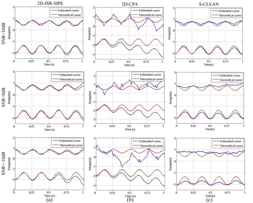
Sensors 2020, 20, 4382                                                                              2 of 16

the design of the radar system and limiting its practicality in reality. In order to solve these problems,
a sparse frequency band (SFB) signal has been developed, including a sparse orthogonal frequency
division multiplexing (OFDM) signal and a sparse stepped-frequency signal [7,8]. Only transmitting
part of the full frequency band (FFB), the SFB signal can effectively avoid certain interference frequency
bands and reduce the data sampling amount, thereby improving the anti-jamming ability of the radar
system and decreasing the operation burden of the radar hardware. However, the SFB signal severely
challenges the traditional micro-motion curve extraction algorithms. Hence, it is of great significance
to study the micro-motion extraction in SFB.
      For the SFB signal, the reconstruction of HRRP is essential. The existing sparse reconstruction
methods can be classified into four main categories. The first is nonlinear filtering represented by
sequence CLEAN (S-CLEAN) [9,10]. It suppresses the high grating and side lobes of the pulse response
function by remaining the peak value of the main lobe. The second is a bandwidth extrapolation
(BWE) algorithm, such as the Burg algorithm [11,12]. This kind of method usually uses the linear
prediction model to fit observation data, then adopts the spectrum estimation method to estimate
the model parameters, and improves resolution through aperture extrapolation. The third is the
parametric spectrum estimation technique, including the RELAX algorithm [13,14]. This type of
algorithm establishes a parametric model for the echo signal, and precisely estimates the positions
and amplitudes of the scattering centers through spectrum estimation so as to achieve high-resolution
imaging. However, the above algorithms are all easily affected by noise and model errors, so the
sparse reconstruction algorithm based on compressive sensing (CS) theory has been proposed in recent
years. This kind of algorithm fulfills sparse data reconstruction by solving an l1 -norm optimization
problem, and thus is highly robust against noise [15,16]. When it comes to the micro-motion target,
the 2-D coupling problem exists in the echo signal duo to micro-motion. Thus, if the 2-D joint
micro-motion parameter estimation can be achieved simultaneously with sparse reconstruction, higher
accuracy in estimation and stronger robustness can be guaranteed. However, by implementing sparse
reconstruction in a single dimension, the above four types of methods fail to make the most of the
2-D coupling information and the 2-D coherent accumulation gain of the echo signal, which adversely
affects the accuracy of signal reconstruction and parameter estimation as well as the robustness
against noise.
      Inspired by the above problems, this paper presents a 2-D joint sparse reconstruction and
micro-motion parameter estimation (2D-JSR-MPE) algorithm aimed at the SFB signal. In this technique,
a novel 2-D joint sparse reconstruction signal model combined with a segmented micro-motion
characteristic parameter dictionary is established, in which the piecewise processing effectively reduces
the model complexity of ballistic target. Based on this, a 2D-JSR-MPE optimization function is developed
by means of the CS sparse representation, transforming the sparse reconstruction and parameter
estimation into solving a sparsity-driven optimization problem with l1 -norm. With the accommodation
of the improved orthogonal matching pursuit (OMP) algorithm [17], micro-motion parameter estimation
and sparse reconstruction can be simultaneously realized, thereby the high-precision HRRP and
micro-motion curve can be obtained. Two-dimensional joint processing makes it possible to prevent the
interference of the sparse reconstruction error in micro-motion parameter estimation, thus effectively
avoiding the adverse effect of error transmission. The proposed algorithm estimates the micro-motion
parameters by processing the phase information, so the estimation accuracy can reach the level of
half a wavelength. Moreover, since the 2-D joint processing makes the most of the 2-D coupling
information and 2-D coherent accumulation gain of the echo signal, and the SFB signal performs well in
anti-jamming with low computational complexity, the proposed algorithm has the advantages of high
accuracy, strong robustness, good practicality and low operational burden. Abundant experimental
results corroborate the superiority of the proposed algorithm.
      This paper is organized as follows. Section 2 introduces the 2D-JSR-MPE signal model of the
ballistic target. Section 3 explicates the 2D-JSR-MPE algorithm. Section 4 provides the experimental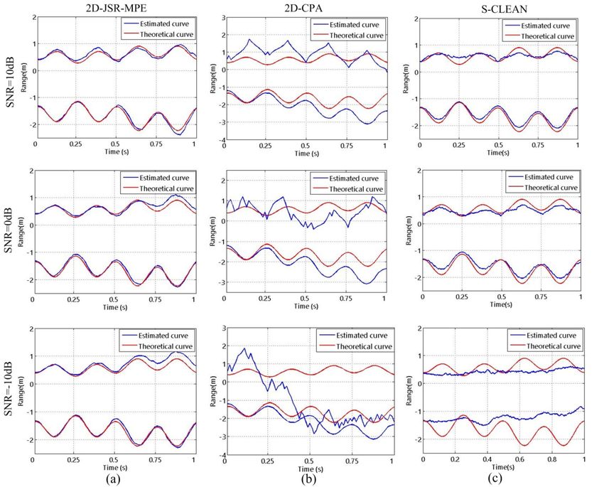
Sensors 2020, 20, 4382 3 of 16
Sensors 2020, 20, x FOR PEER REVIEW 3 of 15
results to illustrate the effectiveness of the proposed algorithm. The paper ends with a brief conclusion
inSignal
2. SectionModel
5.
2. Signal
2.1. Model
The Micro-Motion Model of Ballistic Target
TheMicro-Motion
2.1. The micro-motion model
Model of ballistic
of Ballistic Target target is shown in Figure 1a. ( x , y , z ) is the radar
coordinate system and model
The micro-motion ( X , Y , of
Z ) ballistic
are thetarget
targetisbody
shown coordinate
in Figure system.
1a. (x, y,RLOS is the
z) is the radarradar line of
coordinate
sight,
systemandandthe(X,elevation
Y, Z) are theangle andbody
target the azimuth
coordinate angle of RLOS
system. RLOSare is the and βline
α radar , respectively.
of sight, andThe the
elevation model
geometry angle and the azimuth
of ballistic target is angle
shownof RLOS
in Figure α and
are1b. β, respectively.
H denotes the heightTheofgeometry r refers
the cone, model of
ballistic
to targetofisthe
the radius shown
bottom,in Figure
and d 1b. H denotes
represents thethe height between
distance the rmass
of the cone, refers to theand
center radius of the
the top of
bottom,
the Ford represents
cone.and the ballistic thecone
distance
target between
model the mass center
established in and
this the top of
paper, the cone.
there For the
are three ballistic
equivalent
cone targetcenters
scattering model on established
the targetin[2],
thisnamely p1 , pare
paper, there 2 and p3 in Figure 1b. When moving in precession,
three equivalent scattering centers on the target [2],
namely p , p 2
the target1 makes and p 3 in
a spin Figure 1b. When moving
motion on its axis of symmetry in precession, the target
at an angular makes of
velocity a spin
ωs , motion
and makeson its
a
axis of symmetry at an angular velocity of ωs , and makes a conic motion on the conic axis OM at an
conic motion on the conic axis OM at an angular velocity of ωc . The precession angle is θ . When the
angular velocity of ωc . The precession angle is θ. When the target moves in nutation, on the basis
target moves in nutation, on the basis of precession, the cone axis of the target oscillates in accordance
of precession, the cone axis of the target oscillates in accordance with the sine wave within a certain
with the sine wave within a certain range. The oscillation angle is κ ( t m ) = δ sin (ω v t m ) ; δ and ωv
range. The oscillation angle is κ(tm ) = δ sin(ωv tm ); δ and ωv stand for the maximum amplitude and
stand for the
the angular maximum
velocity amplitude
of oscillation, and the angular
respectively. velocity
Given that of oscillation,
the ballistic respectively.
cone target studied inGiven that
this paper
the ballistic cone target
is axisymmetric, its spinstudied
motionindoes this not
paper is axisymmetric,
affect the radar echoitsofspin motionand
the target doesis not affect not
therefore the radar
taken
echo of the target
into consideration. and is therefore not taken into consideration.
Ballistic target
Figure 1. Ballistic target model:
model: (a)
(a) Micro-motion
Micro-motion model;
model; (b)
(b) Geometry
Geometry model.
model.
In this
In this paper,
paper, it
it is
is assumed
assumed that
that the
the translational
translational motion
motion ofof the
the target
target has
has been
been compensated,
compensated,
then the instantaneous radial distance between the kth scattering center and the radar
then the instantaneous radial distance between the k th scattering center and the radar can be calculated
can be
by the projection
calculated from the kth
by the projection scattering
from center
the k th to RLOS
scattering center to RLOS
) =Y
rk (trmk ()t m= Yk sin γ ( t ) + Z k cos γ ( t mt) +) R+0 R (1)
k sin γ(tmm ) + Z k cos γ( m 0 (1)
where R0 represents the distance from the mass center of target to the radar; γ ( t m ) denotes the
where R0 represents the distance from the mass center of target to the radar; γ(tm ) denotes the angle
angle between
between the symmetry
the symmetry axis axis of the
of the target
target andand
RLOSRLOS tm .tmWhen
at at . Whenthe
thetarget
targetmoves
moves in
in precession,
precession,
the cosine of the angle between the symmetry axis of the target and RLOS can be expressed
the cosine of the angle between the symmetry axis of the target and RLOS can be expressed as as (2)
(2)
cos γ (tm ) = cos θ cos(θ + α ) + sin θ sin(θ + α ) cos(ωc tm + ϕ ) (2)
cos γ(tm ) = cos θ cos(θ + α) + sin θ sin(θ + α) cos(ωc tm + ϕ) (2)
where ϕ denotes initial phase. When the target moves in nutation, the cosine of the angle between
where
the ϕ denotes
symmetry initial
axis of the phase.
targetWhen
and RLOSthe targetcan bemoves
expressedin nutation,
as (3) the cosine of the angle between the
symmetry axis of the target and RLOS can be expressed as (3)
cos γ ( tm ) = cos θ cos (θ + α ) cos κ ( tm ) − sin (α + 3θ ) sin κ ( tm )
(3)
cos γ(tm ) = θ θcos (ω(cθtm+) αcos (α [+κ(3θtm))]sin−sin
κ ( t(mα) + 3θ) sin[κ(tm )]]
− sin (θ + α ) cos κ ( tm )
cos
+ sin [cos ) cos
(3)
+ sin θ cos(ωc tm )[cos(α + 3θ) sin[κ(tm )] − sin(θ + α) cos[κ(tm )]]
Assigning (2) or (3) to (1), the theoretical expression of the instantaneous distance between each
scattering center and the radar can be given by (4)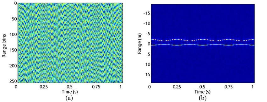
Sensors 2020, 20, 4382 4 of 16
Assigning (2) or (3) to (1), the theoretical expression of the instantaneous distance between each
scattering center and the radar can be given by (4)
rk (tm ) = R0 + Rk (tm ), k = 1, 2, 3
R1 (tm ) = −d cos γ(tm )
(4)
R2 (tm ) = (H − d) cos γ(tm ) − r sin γ(tm )
R3 (tm ) = (H − d) cos γ(tm ) + r sin γ(tm )
where Rk (tm ) represents the instantaneous micro distance of each scattering center. It can be seen that
the instantaneous micro distance of each scattering center changes with time in a form approximating
to the sine wave and includes the target’s motion and geometry parameters.
2.2. D-JSR-MPE Signal Model
It is assumed that the radar transmits a linear frequency modulated (LFM) signal. After
preprocessing such as range compression and de-modulation to the baseband, the received signal of
the kth scattering center can be given by (5) [18]
" #
( fc + fr )
Sk ( fr , tm ) = σk · exp −j4π ·Rk (tm ) (5)
c
where σk represents the scattering coefficient of the kth scattering center; c denotes the light velocity.
From (4), it can be seen that the instantaneous micro distance of each scattering center can be expressed
as a sum of the multi-order Sine functions, but it is complex to cope with such forms in practice. Thus,
underpinned by the idea of piecewise [19], in a short period of time, using a second-order polynomial
model to approximate the instantaneous micro distance of scattering points can reduce the complexity
of the model effectively. Moreover, because of the short dwell time, the second-order polynomial
is accurate enough to fit the instantaneous micro-motion trajectory of the ballistic target, which is
conducive to the subsequent reconstruction of the micro-motion curve. In this paper, the echo signal
is segmented evenly, and the approximate expression of the instantaneous micro distance of the jth
segment of the kth scattering point can be written as (6)
Rkj (tm ) = akj + bkj tm + ckj t2m (6)
where akj , bkj and ckj denote micro-motion parameters. By estimating them accurately, the micro-motion
curve can be reconstructed. Assigning (6) to (5), the jth segmented echo signal can be given by (7)
" #
( fc + fr ) k
Skj ( fr , tm ) = σk · exp −j4π · a j + bkj tm + ckj t2m (7)
c
After sampling processing, the discrete form of (7) can be expressed as (8)
" #
( fc + n∆ f ) k 2
Skj (n, m) = σk · exp −j4π k k
· a j + b j (m∆t) + c j (m∆t) (8)
c
where n refers to the range frequency bin index, and m the azimuth slow time index. The ranges of n
and m are as follows: n ∈ [−N/2 + 1 : N/2 ] and m ∈ [−M/2 + 1 : M/2 ], where N refers to the total
number of the range frequency bin of FFB signal, and M stands for the number of pulses contained in
the jth segmented echo signal. ∆ f corresponds to the range frequency sampling interval, and ∆t the
slow time sampling interval.
Equation (8) is the expression corresponding to the FFB signal. When the range frequency band is
sparse, the geometry model of the SFB signal is shown in Figure 2. It is assumed that the SFB signal
consists of Q sparse subbands, in which the qth subband is Lq in length, running from fq to fq + Lq − 1,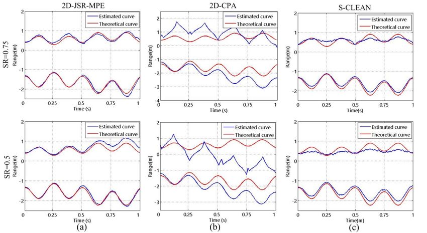
Sensors 2020, 20, 4382 5 of 16
and fq denotes the initial range frequency bin index of the qth subband. It is assumed that the qth
subband signal can be represented by the matrix Skj,q which is Lq × M in size. Then, (8) can be expressed
in the form of matrix, as shown in (9)
h i
Skj = Skj,1 ··· Skj,q ··· Skj,Q (9)
L×M
Q
P
where L = Lq . Assuming that there are a total of K scattering centers in the target, the SBF echo
q=1
Sensors 2020, 20, x FOR PEER REVIEW 5 of 15
signal of the target can be expressed as (10)
Q
where L = Lq . AssumingSthat=thereSare a ·total S j,qK scattering
h i
j
q =1
j,1 · · of · · · S j,Qcenters in the target, the SBF echo (10)
L×M
signal of the target can be expressed as (10)
K
S j ,1 S j , q noise
j = inevitable
Skj,q . ConsideringSthe Sand
P
where S j,q = j , Q L ×combined
M
with (8) and (10),
(10)S j can be
k=1
re-expressed as the Kfollowing matrix form
k
where S j ,q = Sk =1
j ,q . Considering the inevitable noise and combined with (8) and (10), S j can be re-
Sj = Dj
expressed as the following matrix form Fr ·YTj ·FTa + N j (11)
T T
S j = D j Fr ⋅ Y ⋅ F + N j j a (11)
where represents the Hadamard product and D j ∈ CL×ML×denotes
M
the micro-motion parameter matrix
where represents the Hadamard product and D j ∈ denotes the micro-motion parameter
as (12)
matrix as (12)
fc )4π ( Δf + f c ) 4π(4∆πf (+ Δffc+) f c ) 4π ( Δf 4π ) f + fc ) P (M∆t)
∆f+
+ f(c ∆
exp −j 4π (exp
c − j P j ( ∆t ) Pj ( Δ t )
exp −j
exp − j c c P j (
P j (
2∆t 2 Δ )
t ) · · · exp exp
− j −j cPj ( M Δt ) j
c c
.. . .
.
.. . ..
. .
4π ( L Δf + f c ) 4π ( L1 Δf + f c ) 4π ( L1 Δf + f c )
P ( Δt ) exp 4π Pj ( 2 Δt ) ( MfcΔ) t )
L1 ∆ f−+j fc ) 1
= (exp
D 4π − (j L1 ∆ f + fc ) exp − j 4π(L1 ∆Pfj +
P jc(∆t) j exp Pj(M∆t) (12)
D j = exp −jj c −j c c P j (2∆t) · · · exp −j c (12)
c
.. .. ..
..
. 4π ( L Δf + f c !) 4π (.L Δf + f c ) . 4π ( L Δf + f c ) .
exp − j Pj ( Δt ) exp − j Pj ( 2 Δt )! exp − j Pj ( M Δt )
!
4π(L∆ f +cfc )
exp − j 4π(L∆f + fc ) P j c(∆t)
c4π ( L∆ f + f )
P j (2∆t) L ×M
c
c exp −j c ··· exp − j c P j (M∆t)
Pj ( mΔt ) = bj ( mΔt ) + c j ( mΔt )
2 L×M
bj cj
where , m = 1, 2, M , the ranges of and are as follows:
2
where Pb jj ∈ [ −η /)2 : η=/ 2 ]b jand
(m∆t (m∆tc)j ∈+[ −cμj (/m∆t
2 : μ )/ 2, ]m = 1, 2, · · · M, the ranges of b j and c j are as follows:
, in which η and μ should be large enough to ensure
b j ∈ [−η/2 b: η/2 ] cand c j ∈ [−µ/2 : µ/2 ], in which η and µ should be large enough to ensure
j j
that and can include the center frequencies and chirp rates of all sub-segments echoes.
that b j and c j can include the center frequencies and chirp rates of all sub-segments echoes.
Fhr = Fr 0 ; ; Frq ; ; Fr ( Q −1) i represents the partial Fourier dictionary of range dimension,
Fr = Fr0; · · · ; Frq ; · · · ; Fr(Q−1 L×N
) L×N represents the partial Fourier dictionary of range dimension,
Frq =fqfrq ;; ffqrq+Lq −1
f f + L −1 x = f q , f q + 1, , f q + Lq − 1
f rqx = 1, ω rx , , ω ( N −1) x(N−1), x
q q q
, where ,
Frq = frq ; · · · ; frq L ×N , where fxrq = q 1, ωxr , · · ·r , ωr , x = fq , fq + 1, · · · , fq + Lq − 1,
ω r = exp [ − j 2π / N ]. Lq ×N
M ×M
ωr = exp[−j2π/N ]. Fa F∈a ∈ C denotes the standard Fourier dictionary of azimuth dimension,
M×M denotes theM × standard
N
Fourier dictionary of azimuth dimension,
Y j ∈ M×N
whose detailed form is not given here. Y j ∈ C
whose detailed form is not given here. corresponds
corresponds to the
to the 2-D 2-D full-resolution
full-resolution ISAR image
ISAR image
L×M
N
L×M∈
and N j ∈ C j the additive complex Gaussian white noise matrix.
and the additive complex Gaussian white noise matrix.
Figure
Figure 2. 2.The
Thegeometry
geometry model
model of of
SFB signal.
SFB signal.
Equation (11) is the 2D-JSR-MPE signal model proposed in this paper. In the next section, we
Equation (11) is the 2D-JSR-MPE signal model proposed in this paper. In the next section, we will
will explicate the HRRP reconstruction and micro-motion curve estimation of scattering centers based
explicate the HRRP
on the CS theory.
reconstruction and micro-motion curve estimation of scattering centers based on
the CS theory.
3. D-JSR-MPE Algorithm
3.1. The Principle of 2D-JSR-MPE Based on CS
The CS theory points out that by analyzing the sparsity of the echo signal, constructing the
measurement matrix, and using the existing optimization algorithms, the sparse signal can be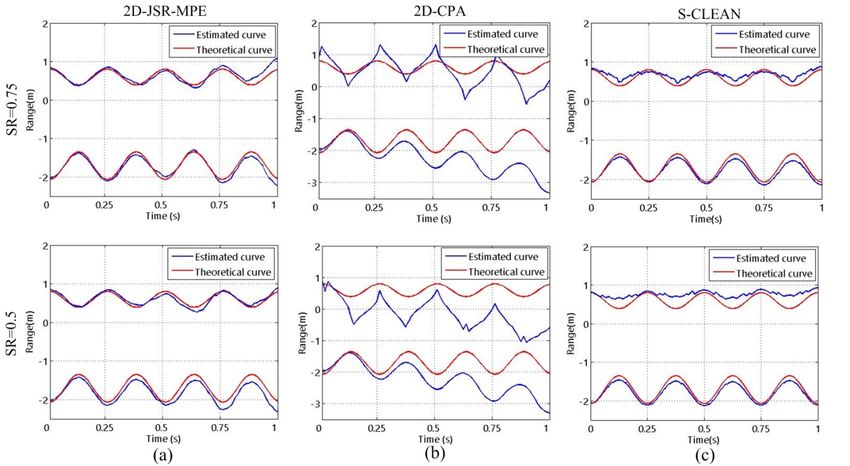
Sensors 2020, 20, 4382                                                                                  6 of 16

3. D-JSR-MPE Algorithm

3.1. The Principle of 2D-JSR-MPE Based on CS
     The CS theory points out that by analyzing the sparsity of the echo signal, constructing the
measurement matrix, and using the existing optimization algorithms, the sparse signal can be
reconstructed with a little data sampling amount. Combined with the derivation in the previous
section, in order to facilitate the construction and solution of the optimization function, the vectorization
operation is carried out for (11)
                                    h i       h                                 i     h i
                                 vec S j = vec D j                  Fr ·YTj ·FTa + vec N j               (13)
                                                                                      h i
where vec[·] refers to the vectorization operation. For clarity, we mark s j = vec S j ∈ C(L·M)×1 ,
                                       h i
y j = vec YTj ∈ C(N·M)×1 , and n j = vec N j ∈ C(L·M)×1 . Based on this, (13) can be expressed as (14)
according to the relationship between vectorization operation and Kronecker product [20–22]

                               s j = G j ·(Fa ⊗ Fr )·y j + n j = G j ·W·y j + n j                        (14)

where ⊗ represents Kronecker product; W ∈ C(L·M)×(N·M) denotes the 2-D joint sparse reconstruction
dictionary, and W = Fa ⊗ Fr . In particular, G j ∈ C(L·M)×(L·M) is a diagonal matrix composed of
all elements in D j as the diagonal elements. Based on the CS theory and (14), we can establish a
2D-JSR-MPE optimization function as (15)

                                     minky j k , st.ks j − G j ·W·y j k < ε j                            (15)
                                                   1                           2

where ε j represents the noise threshold; k·ki denotes the i-norm of vector. According to the CS theory,
2D-JSR-MPE can be realized by solving the l1 -norm optimization problem shown in (15). Therefore,
in the next subsection, we will elucidate an algorithm which can quickly and accurately address the
optimization problem shown in (15).

3.2. 2D-JSR-MPE Based on the Improved OMP Algorithm
     Due to the large size of G j ·W, it is difficult for common algorithms to solve (15). In this subsection,
via fast Fourier transform (FFT), the improved OMP algorithm is employed to jointly realize HRRP
reconstruction and micro-motion curve estimation. The improved OMP algorithm mainly includes the
following four steps:

(1)   Micro-motion curve parameters estimation. Firstly, the micro-motion curve parameters of the
      first scattering center in s j are estimated by (16)

                                         D                     E              H
                                             a1j , b1j , c1j       = max H j ·W s j                      (16)

      where H j = A j G j , and A j ∈ C(L·M)×(L·M) is a diagonal matrix composed of all elements in a j
      as diagonal elements as (17)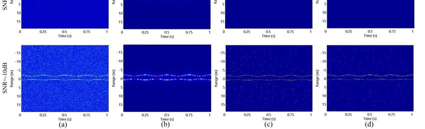
Sensors 2020, 20, 4382 7 of 16
exp −j 4π(∆ f + fc ) a j
4π(∆ f + fc )
4π(∆ f + fc )
c exp − j c a j ··· exp −j c a j
. .. ..
.. ..
. . .
exp − j 4π(L1 ∆ f + fc ) a
4π(L1 ∆ f + fc )
4π(L1 ∆ f + fc )
a j = c j exp −j c aj · · · exp − j c a j
(17)
.. .. .. ..
. . . .
! ! !
4π(L∆ f + fc ) 4π(L∆ f + fc ) 4π(L∆ f + fc )
exp −j aj exp −j aj ··· exp −j aj
c c c
L×M
For solving (16), the traditional method needs to assign all values of a1j , b1j , c1j to H j , respectively,
the computational complexity of each iteration is O NM2 L , which greatly increases the computational
amount. In this paper, FFT is introduced into the process of solving a1j , b1j , c1j
n o
U = FFT2 S j Dj (18)
where FFT2{·} represents the 2-D fast Fourier transform (2D-FFT). Based on (18), â1j , b̂1j , ĉ1j , the optimal
estimation of a1j , b1j , c1j , can be determined by searching the maximum value of U. Then, the basis
matrix corresponding to SFB Φ j = H j,hâ1 ,b̂1 ,ĉ1 i can be constructed by â1j , b̂1j , ĉ1j , and the homologous
j j j
basis matrix with respect to FFB established as ΦFFB
j
.
(2) Scattering center estimation. After obtaining Φ j , the weighted least square estimation (WLSE)
method is adopted to estimate the principal component of the scattering centers in y j , and the
−1
1
corresponding scattering coefficient is Ψ̂ j = Ψ̂ j = ΦH j
Φ j ΦH S . On this basis, we can
j j
^
reconstruct the corresponding SFB observation data S j = Φ j Ψ̂ j .
¯ ^
(3) Residual signal estimation. First, the residual SFB signal S j is calculated by subtracting S j from
¯ ^
S j , i.e., S j = S j − S j . Then, according to step 1 and step 2, the parameter estimation and
¯
scattering center extraction of the principle component signal in S j are carried out. The estimated
micro-motion curve parameters are â2j , b̂2j , ĉ2j . In this case, â2j , b̂2j , ĉ2j are used to update the
basis matrix to Φ j = H j,hâ1 ,b̂1 ,ĉ1 i , H j,hâ2 ,b̂2 ,ĉ2 i , and the scattering coefficients are estimated as
j j j j j j
−1
1 2
Ψ̂ j = Ψ̂ j ; Ψ̂ j = ΦH j
Φ j ΦH j j
S . It should be noted that the scattering coefficient of the
principal component signal estimated in the first time and ΦFFB
j
are also updated here.
¯
(4) Iterative operation. Repeat Step 2 and Step 3 until kS j k2 < ε j is met.
Through the above processing, the micro-motion curve of the kth scattering center of the jth
segment can be reconstructed by (19)
R̂kj (tm ) = âkj + b̂kj tm + ĉkj t2m (19)
Moreover, the reconstructed HRRP of the jth segment can be obtained using range inverse
^ FFB
FFT (IFFT) for the reconstructed FFB signal S j = ΦFFB
j
Ψ̂ j . The final reconstructed HRRPs and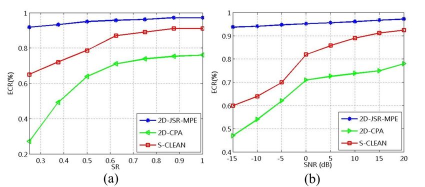
Sensors 2020, 20, 4382                                                                                                       8 of 16

micro-motion curves can be obtained by splicing and integrating the processing results of each
subsegment. Through 2-D joint processing, sparse reconstruction and micro-motion parameter
estimation are carried out simultaneously, which avoids the cascaded error transfer resulting from
“reconstruction first and then estimation”, thus improving the accuracy and robustness of parameter
estimation. Since the proposed algorithm taps the phase information to estimate the micro-motion
parameters, the estimation accuracy can reach the level of half a wavelength, rendering the proposed
algorithm highly accurate in terms of parameter estimation.
     The computational complexity of the proposed algorithm mainly arises from the FFT operation
in Step 1 and the matrix inversion operation
                                         !     in Step 2. The computational complexity of the matrix
                                    K
                                       k3 , which can be neglected since there are only a few equivalent
                                    P
inversion operation in Step 2 is O
                                           k=1
scattering centers for the ballistic target studied in this paper. Therefore, it is Step 1 that mainly
determines the complexity of the proposed algorithm, which can be expressed by the number of complex
multiplications [23]. It can be seen from (18) that 2D-FFT is employed to estimate the                      micro-motion
parameters
Sensors 2020, 20,ofx FOR
                     eachPEERsubsegment.
                                   REVIEW        The computational complexity of 2D-FFT is O M·N log2 (M·N                  8 of )15,
and the search ranges of b j and c j are η and µ, respectively, so the computational complexity
                      ( Jeach                           ) ) . Through
                                  ⋅ M ⋅ N log2 (isMO⋅ Nη·µ·M·N
                          ⋅η ⋅ μsubsegment

algorithm is Oto
corresponding                                                    log2 (FFT
                                                                        M·Nand    Hadamard
                                                                             ) . Given that theproduct,   the computational
                                                                                                 echo signal   is divided into

               of each iteration of the proposed algorithm O ( M ⋅ N log2 ( M ⋅ N ) ) is much smaller

Jcomplexity
  segments, the       total  computational         complexity    of  the proposed   algorithm   is O  J·η·µ·M·N   log  2 ( M·N   )
                                                                                                                             than.
Through FFT and Hadamard product, the computational complexity of each iteration of                           the   proposed
that of direct
algorithm         matrix
              O M·N       logoperation      (        )
                                             O NM 2 L , so the efficiency of the 2-D joint processing algorithm
                               2 (M·N ) is much smaller than that of direct matrix operation O NM L , so the

                                                                                                                    2

                                                                                                                              can
efficiency   of the
be effectively         2-D jointby
                    improved         processing     algorithm can be effectively improved by fast operation.
                                        fast operation.
      In order to describe the proposed  proposed algorithm
                                                       algorithm clearly,
                                                                    clearly,aaflowchart
                                                                               flowchartisisgiven
                                                                                             givenininFigure
                                                                                                        Figure3.3.

                                            Figure 3. Flowchart of 2D-JSR-MPE.

4. Experiments and Analyses
4. Experiments and Analyses
     The geometry model of the ballistic target shown in Figure 1b is adopted in this simulation
     The geometry model of the ballistic target shown in Figure 1b is adopted in this simulation
experiment, and the main simulated target and radar system parameters are shown in Tables 1 and 2,
experiment, and the main simulated target and radar system parameters are shown in Tables 1 and
respectively. In this experiment, three comparison algorithms are employed to illustrate the advantages
2, respectively. In this experiment, three comparison algorithms are employed to illustrate the
of the proposed algorithm. The ‘zero-padding FFT (ZP-FFT)’ method [8] carries out a zero padding
advantages of the proposed algorithm. The ‘zero-padding FFT (ZP-FFT)’ method [8] carries out a
zero padding operation on the part of the vacant frequency band, and obtains the range profiles of
the scattering centers through range IFFT. For the ‘S-CLEAN’ method, the HRRPs of the scattering
centers are reconstructed by the S-CLEAN algorithm [10], and then the micro-motion curve is
extracted by the traditional PDR algorithm. The ‘2-D cascaded processing algorithm (2D-CPA)’ uses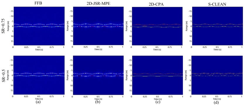
Sensors 2020, 20, 4382 9 of 16
operation on the part of the vacant frequency band, and obtains the range profiles of the scattering
centers through range IFFT. For the ‘S-CLEAN’ method, the HRRPs of the scattering centers are
reconstructed by the S-CLEAN algorithm [10], and then the micro-motion curve is extracted by
the traditional PDR algorithm. The ‘2-D cascaded processing algorithm (2D-CPA)’ uses the OMP
algorithm [17] to reconstruct HRRP in the range dimension first, and then superimposes the target
support area along the range bin. For the superimposed one-dimension (1-D) vector, the modified
discrete chirp Fourier transform (MDCFT) [24] is utilized to estimate the parameters and reconstruct
the micro-motion curve in the azimuth dimension. With respect to the proposed algorithm, for clarity,
we name it as ‘2D-JSR-MPE’. It is worth noting that the HRRPs obtained by ZP-FFT have high gating
and side lobes, so ZP-FFT is not applied to the subsequent estimation of micro-motion parameters
in this experiment. In what follows, the effectiveness and superiority of the proposed algorithm
are demonstrated by the experimental results obtained by the three comparison algorithms and the
proposed algorithm at different signal to noise ratios (SNRs) and sparse rates (SRs).
Table 1. Main simulated parameters of the ballistic target.
Parameters Values
Height of the target 4.0 m
Distance between the mass center and the top of the target 2.7 m
Radius of the bottom 0.3 m
Spinning frequency 2 Hz
Coning frequency 4 Hz
Oscillating frequency 1 Hz
Precession angle 10◦
Table 2. Main simulated parameters of the radar system.
Parameters Values
Carrier frequency 10 GHz
Bandwidth 1 GHz
Pulse repetition frequency 4 kHz
Coherent processing interval 1s
First, the precession motion of the target is studied, and the experiment is carried out at SNR = 10 dB.
Figure 4a shows the FFB echo waveform in range-frequency and azimuth-time domains at SNR = 10 dB
with its corresponding HRRPs in Figure 4b. It can be seen that due to shielding effect, only one
micro-motion curve corresponding to scattering centers p2 or p3 can be observed [25]. It is widely
acknowledged that the sparse sampling pattern can be classified into two categories: gap missing
sampling (GMS) and random missing sampling (RMS). They are only different in the sampling method,
while identical in the subsequent experimental processing. The SFB signal (such as the sparse OFDM
signal) is usually transmitted in the form of GMS. Therefore, in this experiment, we use GMS to
illustrate the performance of the algorithms. In addition, two kinds of SRs are set, SR1 = 0.75 and
SR2 = 0.5. The range dimension sampling points corresponding to SR1 and SR2 are three fourths and
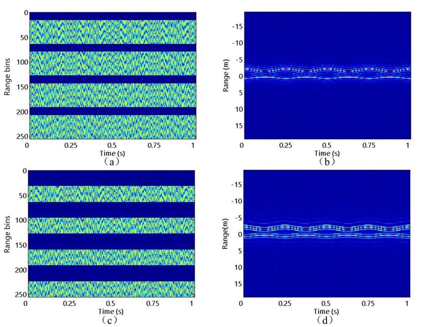
half as many as the FFB sampling points in Figure 4a, respectively. Figure 5 shows the SFB waveforms
at SR1 and SR2 as well as the HRRPs obtained by ZP-FFT. As shown in Figure 5b,d, the HRRPs
obtained by ZP-FFT have high gating and side lobes with low resolution, which seriously hinders the
follow-up work.
In the following experiment, we study the influence of the SR on the algorithms. When the target
is in precession, the reconstructed results of HRRP obtained by 2D-JSR-MPE, 2D-CPA and S-CLEAN
in the case of SR1 and SR2 are shown in Figure 6. It can be seen that in the case of SR1, all three
algorithms can reconstruct good HRRPs. However, at SR2, due to the influence of high grating and side
lobes, severe errors occur in the HRRPs reconstructed by S-CLEAN. Figure 7 shows the micro-motion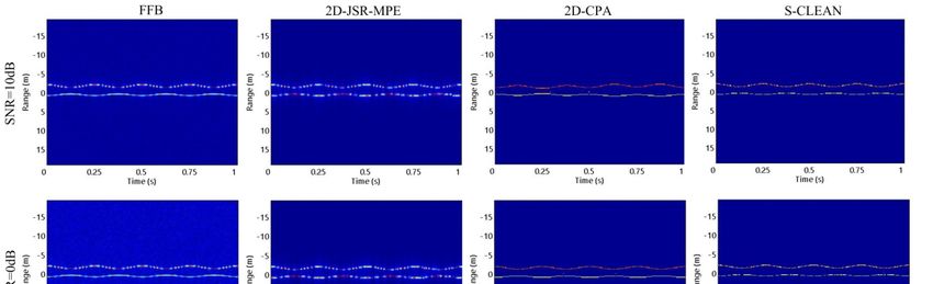
First, the precession motion of the target is studied, and the experiment is carried out at
SNR = 10 dB. Figure 4a shows the FFB echo waveform in range-frequency and azimuth-time domains
at SNR = 10dB with its corresponding HRRPs in Figure 4b. It can be seen that due to shielding effect,
only one micro-motion curve corresponding to scattering centers p2 or p3 can be observed [25]. It
is widely acknowledged that the sparse sampling pattern can be classified into two categories:
Sensors 2020, 20, 4382
gap
10 of 16
missing sampling (GMS) and random missing sampling (RMS). They are only different in the
sampling method, while identical in the subsequent experimental processing. The SFB signal (such
curves
as thereconstructed
sparse OFDMby the three
signal) algorithms
is usually corresponding
transmitted in the form to of
precession at the two
GMS. Therefore, SRs.experiment,
in this Since the
S-CLEAN
we use GMS to illustrate the performance of the algorithms. In addition, two kinds of SRs areofset,
method is used to extract the maximum peak point to achieve the suppression high
SR1
grating
= 0.75 and
andside
SR2lobes,
= 0.5. with the decrease
The range in SR,sampling
dimension the error points
arisingcorresponding
from extractingtopeak
SR1point leadsare
and SR2 to three
the
micro-motion
fourths and curve
half asreconstruction
many as the FFB failure. 2D-CPA
sampling fails to
points in make
Figurefull
4a,use of 2-D coupling
respectively. Figureinformation
5 shows the
and 2-D coherent accumulation gain of echo signal due to cascaded processing,
SFB waveforms at SR1 and SR2 as well as the HRRPs obtained by ZP-FFT. As shown in Figure and is prone to the
5b,d,
estimation
the HRRPs error transmission,
obtained by ZP-FFT so its
havereconstruction
high gating andaccuracy is insufficient.
side lobes In contrast,which
with low resolution, 2D-JSR-MPE
seriously
can accurately
hinders reconstruct
the follow-up the micro-motion curve in the same condition.
work.
Sensors 2020, 20, x FOR PEER REVIEW 10 of 15
Figure FFB
4. 4.
Figure situation:
FFB (a)(a)
situation: Echo waveform;
Echo (b)(b)
waveform; HRRPs.
HRRPs.
Figure5. 5.SFB
Figure SFBsituation.
situation.SR1:
SR1: (a)
(a)Echo
Echowaveform;
waveform;(b)
(b)HRRPs
HRRPsobtained
obtainedbybyZP-FFT.
ZP-FFT.SR2:
SR2:(c)(c)Echo
Echo
waveform;
waveform; (d)(d)
HRRPs
HRRPs obtained
obtainedbybyZP-FFT.
ZP-FFT.
InIn
order to study the
the following influence of
experiment, weSNR on the
study the algorithms,
influence ofHRRPs arethe
the SR on reconstructed
algorithms.by 2D-JSR-MPE,
When the target
2D-CPA and S-CLEAN at SNR = −10 dB, 0 dB and 10 dB. The homologous results
is in precession, the reconstructed results of HRRP obtained by 2D-JSR-MPE, 2D-CPA and S-CLEAN are shown in
Figure 8. It can be seen that there are a lot of false points in the HRRPs reconstructed
in the case of SR1 and SR2 are shown in Figure 6. It can be seen that in the case of SR1, all three by 2D-CPA
and S-CLEAN
algorithms canatreconstruct
low SNR, but 2D-JSR-MPE
good succeed at
HRRPs. However, in SR2,
reconstructing
due to the HRRPs
influenceaccurately. Figureand
of high grating 9
reveals the micro-motion curves reconstructed by the three algorithms under the three
side lobes, severe errors occur in the HRRPs reconstructed by S-CLEAN. Figure 7 shows the micro- SNR conditions.
Asmotion
SNR decreases, 2D-CPA and
curves reconstructed byS-CLEAN are seriously
the three algorithms disturbed bytonoise,
corresponding and the
precession at error of the
the two SRs.
Since the S-CLEAN method is used to extract the maximum peak point to achieve the suppression of
high grating and side lobes, with the decrease in SR, the error arising from extracting peak point leads
to the micro-motion curve reconstruction failure. 2D-CPA fails to make full use of 2-D coupling
information and 2-D coherent accumulation gain of echo signal due to cascaded processing, and is
prone to the estimation error transmission, so its reconstruction accuracy is insufficient. In contrast,in the case of SR1 and SR2 are shown in Figure 6. It can be seen that in the case of SR1, all three
algorithms can reconstruct good HRRPs. However, at SR2, due to the influence of high grating and
side lobes, severe errors occur in the HRRPs reconstructed by S-CLEAN. Figure 7 shows the micro-
motion curves reconstructed by the three algorithms corresponding to precession at the two SRs.
Since the S-CLEAN method is used to extract the maximum peak point to achieve the suppression of
Sensors 2020, 20, 4382 11 of 16
high grating and side lobes, with the decrease in SR, the error arising from extracting peak point leads
to the micro-motion curve reconstruction failure. 2D-CPA fails to make full use of 2-D coupling
information and
reconstructed 2-D coherent
micro-motion accumulation
curves increases gain of echoHowever,
gradually. signal duecompared
to cascaded processing,
with the aboveand twois
prone to thealgorithms,
comparison estimation2D-JSR-MPE
error transmission,
can still so its reconstruction
reconstruct accuracy
the accurate is insufficient.
micro-motion curves atIn different
contrast,
2D-JSR-MPE
SNRs. can above
The experiments accurately reconstruct
corroborate the
the good robustness micro-motion
of curve against
the proposed algorithm in the
SR
same
and SNR.condition.
Figure
Figure6. Thereconstructed
6. The reconstructed results
results of HRRP
of HRRP oftarget
of the the target with precession
with precession motionmotion obtained
obtained by
by different
different
algorithmsalgorithms with different
with different SRs at
SRs at SNR = SNR = (a)
10 dB: 10 dB:
FFB(a) FFB situation;
situation; (b) 2D-JSR-MPE;
(b) 2D-JSR-MPE; (c) 2D-CPA;
(c) 2D-CPA; (d) S-
Sensors 2020, 20, x FOR PEER REVIEW 11 of 15
(d) S-CLEAN.
CLEAN.
Figure7.7.The
Figure Thereconstructed
reconstructedresults
resultsofofmicro-motion
micro-motioncurves
curvesofofthe
thetarget
targetwith
withprecession
precessionmotion
motion
obtained by different algorithms with different
obtained by different algorithms with different SRs at SNR = 10 dB: (a) 2D-JSR-MPE; (b) 2D-CPA;
SNR = 10 dB: (a) 2D-JSR-MPE; (b) 2D-CPA; (c)
(c)S-CLEAN.
S-CLEAN.
InInaddition,
order to based
study on
thethe precession
influence motion
of SNR of the
on the target, theHRRPs
algorithms, oscillating motion of the symmetry
are reconstructed by 2D-JSR-
axis
MPE, 2D-CPA and S-CLEAN at SNR = −10 dB, 0 dB and 10 dB. The homologous results arethe
of the target is introduced into the experiment to estimate the micro-motion curves of targetin
shown
with nutation motion. Figures 10 and 11 are the corresponding micro-motion curves reconstructed
Figure 8. It can be seen that there are a lot of false points in the HRRPs reconstructed by 2D-CPA and by
the three algorithms
S-CLEAN at the
at low SNR, buttwo kinds of SRs
2D-JSR-MPE and the
succeed inthree types of SNRs
reconstructing HRRPswhen the targetFigure
accurately. is in nutation.
9 reveals
They suggest that the experimental conclusions drawn in the complex nutation are
the micro-motion curves reconstructed by the three algorithms under the three SNR conditions. the same as those
As
acquired in the precession, which further verify the effectiveness of the proposed
SNR decreases, 2D-CPA and S-CLEAN are seriously disturbed by noise, and the error of the algorithm.
reconstructed micro-motion curves increases gradually. However, compared with the above two
comparison algorithms, 2D-JSR-MPE can still reconstruct the accurate micro-motion curves at
different SNRs. The experiments above corroborate the good robustness of the proposed algorithm
against SR and SNR.the micro-motion curves reconstructed by the three algorithms under the three SNR conditions. As
SNR decreases, 2D-CPA and S-CLEAN are seriously disturbed by noise, and the error of the
reconstructed micro-motion curves increases gradually. However, compared with the above two
comparison algorithms, 2D-JSR-MPE can still reconstruct the accurate micro-motion curves at
different
Sensors 2020, SNRs.
20, 4382 The experiments above corroborate the good robustness of the proposed algorithm
12 of 16
against SR and SNR.
Figure
Figure8. Thereconstructed
8. The reconstructed results
results of HRRP
of HRRP oftarget
of the the target with precession
with precession motionmotion obtained
obtained by
by different
different
algorithmsalgorithms with different
with different SNRs atSNRs SR =(a)0.75:
SR =at0.75: FFB(a) FFB situation;
situation; (b) 2D-JSR-MPE;
(b) 2D-JSR-MPE; (c) 2D-CPA;
(c) 2D-CPA; (d) S-
Sensors
(d) 2020, 20, x FOR PEER REVIEW
S-CLEAN. 12 of 15
CLEAN.
Figure9.9.The
Figure Thereconstructed
reconstructedresults
resultsofofmicro-motion
micro-motioncurves
curvesofofthethetarget
targetwith
withprecession
precessionmotion
motion
obtained
obtainedbybydifferent
different algorithms with different
algorithms with differentSNRs
SNRsatatSR = 0.75:
SR= 0.75: (a) 2D-JSR-MPE;
(a) 2D-JSR-MPE; (b) 2D-CPA;
(b) 2D-CPA; (c) S-
(c)CLEAN.
S-CLEAN.
In addition, based on the precession motion of the target, the oscillating motion of the symmetry
axis of the target is introduced into the experiment to estimate the micro-motion curves of the target
with nutation motion. Figures 10 and 11 are the corresponding micro-motion curves reconstructed
by the three algorithms at the two kinds of SRs and the three types of SNRs when the target is in
nutation. They suggest that the experimental conclusions drawn in the complex nutation are the same
as those acquired in the precession, which further verify the effectiveness of the proposed algorithm.In addition, based on the precession motion of the target, the oscillating motion of the symmetry
axis of the target is introduced into the experiment to estimate the micro-motion curves of the target
with nutation motion. Figures 10 and 11 are the corresponding micro-motion curves reconstructed
by the three algorithms at the two kinds of SRs and the three types of SNRs when the target is in
nutation.
Sensors They
2020, 20, 4382suggest that the experimental conclusions drawn in the complex nutation are the
13 same
of 16
as those acquired in the precession, which further verify the effectiveness of the proposed algorithm.
Figure10.10.The
Figure The reconstructed
reconstructed results
results of micro-motion
of micro-motion curvescurves of thewith
of the target target with motion
nutation nutation motion
obtained
Sensors
by 2020,
obtained20, by
different x algorithms
FOR PEER REVIEW
different with different
algorithms withSRs
different = 10atdB:
at SNRSRs (a) 2D-JSR-MPE;
SNR=10dB: (b) 2D-CPA;
(a) 2D-JSR-MPE; (b) (c) S-CLEAN.
2D-CPA; 13 of 15
(c) S-
CLEAN.
Figure11.11.The
Figure reconstructed
The results
reconstructed of micro-motion
results curvescurves
of micro-motion of the target
of thewith nutation
target with motion obtained
nutation motion
by differentbyalgorithms
obtained with different
different algorithms withSNRs
different = 0.75:
at SRSNRs at (a)
SR 2D-JSR-MPE; (b) 2D-CPA;(c)
= 0.75: (a) 2D-JSR-MPE; S-CLEAN. S-
(b) 2D-CPA;(c)
CLEAN.
For the purpose of analyzing the impact of SR and SNR on the performances of the proposed
algorithm andpurpose
For the the two of
comparison
analyzing algorithms
the impact quantitatively,
of SR and SNRthe
onestimated correct rate
the performances (ECR)
of the of the
proposed
reconstructed micro-motion curve is defined by (20)
algorithm and the two comparison algorithms quantitatively, the estimated correct rate (ECR) of the
reconstructed micro-motion curve is defined
P by (20)
Fr (tm ) − Fe (tm )
t F r ( m)
t − F e ( m)
t
m
ECR = 1 − t P ∗ 100% (20)
ECR = 1 − m
*100%
Fr (tm ) (20)
F t
tm ( )r m
tm
where Fe ( t m ) represents the estimated value of the micro-motion curve and Fr ( t m ) the true value
of the micro-motion curve. Firstly, the influence of SR on the performance of the algorithms is
analyzed. In the case of precession motion, with other conditions unchanged, SR ranges from 0.25 to
1 in step of 0.125 at SNR = 10 dB. Without loss of generality, 40 groups of echo data are collected at
each SR, followed by the reconstruction of their micro-motion curves. After calculating the ECR ofSensors 2020, 20, 4382 14 of 16
where Fe (tm ) represents the estimated value of the micro-motion curve and Fr (tm ) the true value of
the micro-motion curve. Firstly, the influence of SR on the performance of the algorithms is analyzed.
In the case of precession motion, with other conditions unchanged, SR ranges from 0.25 to 1 in step
of 0.125 at SNR = 10 dB. Without loss of generality, 40 groups of echo data are collected at each SR,
followed by the reconstruction of their micro-motion curves. After calculating the ECR of each curve,
the average value of 40 groups of ECRs can be obtained, which is shown in Figure 12a. Compared
Sensors 2020, 20, x FOR PEER REVIEW 14 of 15
with the other two algorithms, the proposed one has higher ECRs at all SRs.
Figure 12. ECRs obtained
Figure12. obtained by
bydifferent
differentalgorithms:
algorithms:(a)(a) Different
Different algorithms
algorithms with
with different
different SRsSRs at
at SNR
= 10=dB;
SNR 10 (b)
dB;Different
(b) Different algorithms
algorithms withwith different
different SNRsSNRs at =SR
at SR = 0.75.
0.75.
Finally
Finallycomes
comesthe
theanalysis
analysisofofthe
theinfluence
influenceofofSNR
SNRononthe thealgorithms’
algorithms’performance.
performance.Assuming
Assuming
other
other conditions remain unchanged, the robustness of the algorithms against noise is analyzedwith
conditions remain unchanged, the robustness of the algorithms against noise is analyzed with
SRSR==0.75
0.75and
andSNR
SNRranging from−15
rangingfrom −15toto20
20dB
dBininstep
stepofof55dB.
dB.TheTheaverage
averageECR
ECRisiscalculated
calculatedbybythe
the
same
samemethod,
method,andandthe
theresult
resultisisshown
shownininFigure
Figure12b.
12b.ItItcan
canbebeseen
seenthat
thatthe
theECRs
ECRsofofthe
theproposed
proposed
algorithm
algorithmare
areabove
above90%
90%atatdifferent
differentSNRs,
SNRs,higher
higherthan
thanthose
thoseofofthe
theother
othertwo
twoalgorithms.
algorithms.This
Thisserves
serves
asasconvincing proof of the good robustness of the proposed algorithm against
convincing proof of the good robustness of the proposed algorithm against noise. noise.
5. Conclusions
5. Conclusions
This paper proposes a novel 2D-JSR-MPE algorithm. Through piecewise processing, we establish
This paper proposes a novel 2D-JSR-MPE algorithm. Through piecewise processing, we
the 2-D joint sparse reconstruction signal model and the target’s micro-motion characteristic parameter
establish the 2-D joint sparse reconstruction signal model and the target’s micro-motion characteristic
dictionary, in which the idea of piecewise effectively reduces the model complexity of ballistic target.
parameter dictionary, in which the idea of piecewise effectively reduces the model complexity of
Based on the CS theory, an improved OMP algorithm is employed to solve a sparse optimization
ballistic target. Based on the CS theory, an improved OMP algorithm is employed to solve a sparse
problem with l1 -norm. With the help of 2-D joint processing, the precise reconstruction of HRRP and
optimization problem with l1 -norm. With the help of 2-D joint processing, the precise reconstruction
micro-motion curve can be realized simultaneously, thereby avoiding the error transmission between
of HRRP and micro-motion curve can be realized simultaneously, thereby avoiding the error
HRRP reconstruction and micro-motion parameters estimation. Making full use of the 2-D coupling
transmission between HRRP reconstruction and micro-motion parameters estimation. Making full
information and 2-D coherent accumulation gain of echo signal, the proposed algorithm can accurately
use of the 2-D coupling information and 2-D coherent accumulation gain of echo signal, the proposed
reconstruct the micro-motion curve of the ballistic target on phase accuracy. Extensive experimental
algorithm can accurately reconstruct the micro-motion curve of the ballistic target on phase accuracy.
results demonstrate that the proposed algorithm can be implemented with high accuracy and strong
Extensive experimental results demonstrate that the proposed algorithm can be implemented with
robustness at different SNRs and SRs. Further efforts to improve the performance of our work in this
high accuracy and strong robustness at different SNRs and SRs. Further efforts to improve the
paper in the case of sparse frequency band and sparse aperture (SFB-SA) echo signal of ballistic target
performance of our work in this paper in the case of sparse frequency band and sparse aperture (SFB-
are underway.
SA) echo signal of ballistic target are underway.
Author Contributions:J.W.
AuthorContributions: is is
J.W. responsible forfor
responsible all all
the the
theoretical work,
theoretical the implementation
work, of theofexperiments
the implementation and
the experiments
the writing of the manuscript. L.Z., S.S. and H.L. revised the manuscript. All authors have read and agreed to the
and the writing of the manuscript. L.Z., S.S. and H.L. revised the manuscript. All authors have read and agreed
published version of the manuscript.
to the published version of the manuscript.
Funding: This work was supported by the National Natural Science Foundation of China with grant numbers
Funding:and
61771372 This work was
61771367, thesupported by the National
National Science Foundation Natural Science Foundation
for Distinguished of China with
Young Scholars with grant
grant number
numbers
61525105,
61771372and
andthe Fund forthe
61771367, Foreign Scholars
National in University
Science FoundationResearch and Teaching
for Distinguished Programs
Young (thewith
Scholars 111 grant
Project) with
number
grant number B18039.
61525105, and the Fund for Foreign Scholars in University Research and Teaching Programs (the 111 Project)
with grant number B18039.
Acknowledgments: The authors thank the anonymous reviewers for their valuable comments to improve the
paper quality.
Conflicts of Interest: The authors declare no conflict of interest.Sensors 2020, 20, 4382 15 of 16
Acknowledgments: The authors thank the anonymous reviewers for their valuable comments to improve the
paper quality.
Conflicts of Interest: The authors declare no conflict of interest.
References
1. Chen, V.C.; Li, F.; Ho, S.S.; Wechsler, H. Micro-Doppler effect in radar: Phenomenon, model, and simulation
study. IEEE Trans. Aerosp. Electron. Syst. 2006, 42, 2–21. [CrossRef]
2. Gao, H.; Xie, L.; Wen, S.; Kuang, Y. Micro-Doppler Signature Extraction from Ballistic Target with
Micro-Motions. IEEE Trans. Aerosp. Electron. Syst. 2010, 46, 1969–1982. [CrossRef]
3. Xing, Y.; You, P.; Yong, S. Parameter Estimation of Micro-Motion Targets for High-Resolution-Range Radar
Using Online Measured Reference. Sensors 2018, 18, 2773. [CrossRef] [PubMed]
4. Wu, Y.; Lu, H.; Zhao, F.; Zhang, Z. Estimating Shape and Micro-Motion Parameter of Rotationally Symmetric
Space Objects from the Infrared Signature. Sensors 2016, 16, 1722. [CrossRef] [PubMed]
5. Camp, W.W.; Mayhan, J.T.; O’Donnell, R.M. Wideband radar for ballistic missile defense and range-doppler
imaging for satellites. Linc. Lab. J. 2000, 12, 267–280.
6. Liu, Y.; Zhu, D.; Li, X.; Zhuang, Z. Micromotion characteristic acquisition based on wideband radar phase.
IEEE Trans. Geosci. Remote Sens. 2014, 52, 3650–3657. [CrossRef]
7. Su, X.; Liu, Z.; Chen, X.; Wei, X. Closed-Form Algorithm for 3-D Near-Field OFDM Signal Localization under
Uniform Circular Array. Sensors 2018, 18, 226. [CrossRef]
8. Zhang, L.; Qiao, Z.; Xing, M.; Li, Y.; Bao, Z. High-resolution ISAR imaging with sparse stepped-frequency
waveforms. IEEE Trans. Geosci. Remote Sens. 2011, 49, 4630–4651. [CrossRef]
9. Bose, R.; Freeman, A.; Steinberg, B.D. Sequence CLEAN: A modified deconvolution technique for microwave
images of contiguous targets. IEEE Trans. Aerosp. Electron. Syst. 2002, 38, 89–97. [CrossRef]
10. Martorella, M.; Acito, N.; Berizzi, F. Statistical CLEAN Technique for ISAR Imaging. IEEE Trans. Geosci.
Remote Sens. 2007, 45, 3552–3560. [CrossRef]
11. Li, H.J.; Farhat, N.H.; Shen, Y. A new iterative algorithm for extrapolation of data available in multiple
restricted regions with applications to radar imaging. IEEE Trans. Antennas. Propag. 1987, 35, 581–588.
12. Gupta, I.; Beals, M.; Moghaddar, A. Data extrapolation for high resolution radar imaging. IEEE Trans.
Antennas. Propag. 1994, 42, 1540–1545. [CrossRef]
13. Huan, S.; Zhang, M.; Dai, G.; Gan, H. Low Elevation Angle Estimation with Range Super-Resolution in
Wideband Radar. Sensors 2020, 20, 3104. [CrossRef] [PubMed]
14. Lane, R.O.; Copsey, K.D.; Webb, A.R. A Bayesian approach to simultaneous autofocus and super-resolution.
Proc. Spie Int. Soc. Opt. Eng. 2004, 5427, 133–142.
15. Rauhut, H.; Schnass, K.; Vandergheynst, P. Compressed sensing and redundant dictionaries. IEEE Trans.
Inf. Theory 2008, 54, 2210–2219. [CrossRef]
16. Chung, H.; Park, Y.M.; Kim, S. Wideband DOA Estimation on Co-prime Array via Atomic Norm Minimization.
Sensors 2020, 13, 3235. [CrossRef]
17. Zhang, L.; Duan, J.; Qiao, Z.J.; Xing, M.; Bao, Z. Phase adjustment and isar imaging of maneuvering targets
with sparse apertures. IEEE Trans. Aerosp. Electron. Syst. 2014, 50, 1955–1973. [CrossRef]
18. Shao, S.; Zhang, L.; Liu, H.; Zhou, Y. Accelerated translational motion compensation with contrast
maximisation optimisation algorithm for inverse synthetic aperture radar imaging. IET Radar Sonar
Navig. 2019, 13, 316–325. [CrossRef]
19. Voros, J. Modeling and parameter identification of systems with multisegment piecewise-linear characteristics.
IEEE Trans. Autom. Control 2002, 47, 184–188. [CrossRef]
20. Jahromi, M.J.; Kahaei, M.H. Two-dimensional iterative adaptive approach for sparse matrix solution.
Electron. Lett. 2014, 50, 45–47. [CrossRef]
21. Duarte, M.F.; Baraniuk, R.G. Kronecker Compressive Sensing. IEEE Trans. Image Process. 2012, 21, 494–504.
[CrossRef] [PubMed]
22. Shao, S.; Zhang, L.; Liu, H. High-resolution ISAR imaging and motion compensation with 2-D joint sparse
reconstruction. IEEE Trans. Geosci. Remote Sens. 2020, 1–21. [CrossRef]
23. Shao, S.; Zhang, L.; Liu, H.; Zhou, Y. Spatial-variant contrast maximization auto focus algorithm for ISAR
imaging of maneuvering targets. Sci. China Inf. Sci. 2019, 62, 37–39. [CrossRef]You can also read