Source Guided Speech Synthesis for Speech-To-Speech Translation Using FastSpeech 2 - Maastricht University
←
→
Page content transcription
If your browser does not render page correctly, please read the page content below
Source Guided Speech Synthesis for
  Speech-To-Speech Translation Using FastSpeech 2
                                                               Pedro Antonio Jeuris
                                           Department of Data Science and Artificial Intelligence
                                                          Maastricht University
                                                       Maastricht, The Netherlands

   Abstract—The need for Speech-to-Speech translation tools in
the modern society increases to overcome the language barrier.
While certain tools already exist, they do not take the prosody or
intonation from the source speaker into account for the speech
synthesis. As a result, the translated speech might not encapsulate
the message from the source speaker as the prosody might be on
a different word. This could affect the way the other interlocutor
perceives what was said. To solve this issue, the speech synthesiser
would ideally take the source speech into consideration. However,              Fig. 1. Conventional (black, full lines) and proposed (blue, dashed lines)
only a limited amount of datasets containing speech aligned audio              additions to the pipelines
clips in different language are available. In this research a dataset
of German, English audio pairs is created. Furthermore, this
dataset is applied to multiple adaptations of the Fastspeech 2
Text-To-Speech model. Using this additional input has resulted
in speech with pitch characteristics closer to the target speaker
and a higher predicted naturalness over the baseline model.
   Index Terms—Speech-to-Speech translation, Text-to-Speech,
Speech synthesis, Dataset creation
                                                                               sarcasm is used or other information that may not be apparent
                          I. I NTRODUCTION                                     from a text representation.
                                                                               The most trivial use case for Speech-to-Speech Translation,
   As the world becomes more and more connected, both                          where ideally there would be no loss of prosody, is a con-
online and offline, the need for language translation systems                  versation between two (or more) people who do not speak the
rises to overcome the large existing language barrier [1], [2].                same language. An application that tries to solve this is Jibbigo
In the past few years the advancements made within the                         [5] but there is no mention of perseverance of prosody from
Machine Translation domain have been significant. Computers                    source to target audio. The communication app Skype also has
have become better at translating text between two languages                   a built in translation function [6]. Their pipeline makes use of
and can even translate speech to text in another language                      a cascade model as presented earlier.
by using a single model [3]. To solve the Speech-to-Speech                     The goal of this research is to investigates how information
Translation (S2ST) problem, in which a spoken phrase needs                     such as the source text, pitch or/and energy can be used to
to be instantly translated and spoken aloud in a second                        improve the quality of the generated speech in the target
language, the problem is typically broken into three steps. In                 language. This is done by first collecting a dataset containing
the first step the source audio gets transformed into text by                  aligned audio in the source and target language and their
using a Speech-to-Text (STT) model. The second step uses                       transcriptions. Afterwards adaptations to the input of the TTS
a Text-to-Text translation model to convert the text from the                  model as can be seen in Fig. 1 are made. Multiple adaptations
source language to the target language. The last step takes                    of the TTS model are explored. Each of these adaptations uses
in the translated text as input and synthesises speech in the                  additional information extracted from the source audio to help
target language using a Text-To-Speech (TTS) model. Because                    generating the target audio.
of this concatenation of three models, and the intermediate                    Section II gives an overview of the state of the art and related
text representation there is a loss of information from the                    work on S2ST systems and data sets that can be used. Section
original audio [4]. This information loss mainly consists of                   III talks about the models used in this research and some
speech characteristics such as pitch and energy which are key                  implementation details. Then section IV and V talk about the
elements for prosody. Prosody is essential for a conversation as               acquisition of the dataset and the adaptations of the TSS model
it contains information on the emotional state of the speaker, if              proposed in this paper. The sixth section gives an overview
                                                                               on the preprocessing, data size and evaluation. After this the
  This thesis was prepared in partial fulfilment of the requirements for the
Degree of Bachelor of Science in Data Science and Artificial Intelligence,     last three sections go over the results, a discussion and the
Maastricht University. Supervisors: Dr. Jan Nieheus and Dr. Rico Möckel       conclusion are presented.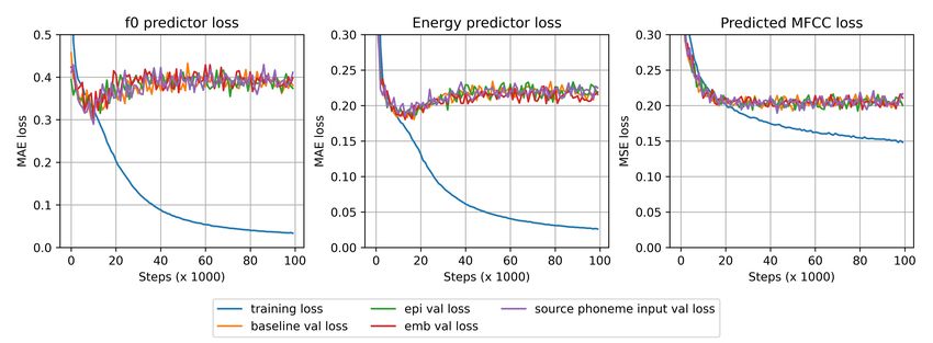
Fig. 2. Fastspeech 2 architecture, figure adapted from [7].Abbreviations: LN layer normalisation; LR: Length Regulator (introduced in the original FastSpeech
paper [8], further information on the embedding, encoder and decoder can also be found in the FastSpeech paper)

         II. S TATE OF THE ART AND RELATED WORK                                 prosody embedding layer they are able to transfer prosodic
                                                                                characteristics between speakers in the same model.
A. S2ST systems
   Modern day Speech-to-Speech-Translation (S2ST) systems                       B. Datasets
such as provided by Microsoft Azure [9] and Skype [6]
make use of a concatenation of state-of-the-art models. As                         Most datasets used in state-of-the-art translation research
mentioned in the introduction this can result in a loss of                      such as LibrivoxDeEn [15], CoVoST2 [16] or MuST-C [17]
information. The oldest pipeline to take additional information,                are focused on Speech-to-Text translation. These datasets only
such as prosody, into account was that of Verbmobile [10].                      contain source audio, transcription and translation in the target
The project was active between 1993 and 2000 and aimed                          language. Furthermore, datasets that contain the audio from
to “support verbal communication with foreign interlocutors                     the target language such as Fisher and CALLHOME Spanish-
in mobile situations” between German, English, and Japanese                     English dataset [18], SP2 speech corpus [19] and the EMIME
[11]. Within the Verbmobile project pitch, energy and other                     Project [20] are either protected behind a paywall or only have
features of speech were used to:                                                a limited amount of samples. This can obstruct research and
1) annotate the generated text with additional information 2)                   development as they are hard to obtain for some people.
use this information to help with the translation 3) apply                         Another option would be to use synthetic data to create the
speaker adaptation [11]. Trying to achieve the same goal, in                    speech from the language that is missing in speech-translation
this paper the source information will be used only to enhance                  data sets. Synthetic speech data has already been successfully
the quality of the generated speech at the end of the pipeline.                 applied to the Speech recognition task [21], [22] where
   Truong Do et al. [12] try to control the prosody in the                      synthetic speech was mixed with existing data to increase the
generated speech by using a prosody estimator. Their prosody                    performance of their models. But Nick Rossenback and his
estimator takes the source text as input and predicts for each                  team also stated that ”TTS outputs are still poor in stability
word an emphasis probability between 0 and 1. They then                         and speaker adaptation capabilities” [21], which makes them
translate this prosody estimation to the target language and use                unusable to train a TTS system on. Especially if prosody is
these values as additional input of their TTS model. Compared                   of importance.
to this work, source information will also be mapped to the
target language but instead of using an intermediate predictor                     Since audio pairs of the same sentences in two languages
the extracted values from the source are used.                                  are needed, this work will build further upon already existing
   The work of RJ Skerry-Ryan Et al. [13] focuses on transfer-                  speech-translation datasets. The missing audio segments will
ring prosody between two speakers within the same language.                     be scraped from the internet and alligned to match the dataset.
By adapting the Tacotron [14] architecture to contain an extra                  This is described in Sec. IV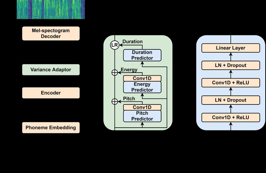
III. T EXT-T O -S PEECH MODELS                                                  TABLE I
                                                                                             C OLLECTED DATA SIZES
   In the TTS pipeline two models are used. A feature
generation model takes the phoneme sequence of the target                                                 German      English
                                                                                     # Audio files        25 635      25 635
sentence as input and outputs the Mel Frequency Cepstral                             # unique Tokens      10 367      9 322
Coefficients (MFCCs). The second model, called the vocoder,                          # Words              49 129      62 961
takes in these MFCCs as input and outputs the generated                              # Speakers           42          29
speech in waveform.                                                                  Duration
                                                                                                          52:30:57    57:20:10
                                                                                     (hh:mm:ss)

   The feature generation model used for this research is
FastSpeech 2 [7]. This model is of particular interest because      as all data used if part of the public domain according to
it has separate predictors for pitch and energy as can be seen in   Librivox.
Fig. 2. The implementation used in this research can be found
in the TensorFlowTTS1 GitHub repository. Compared to the                                  V. P ROPOSED METHODS
original paper, this implementation has made a few changes             To help the TTS model predict the energy and pitch in
such as: 1) The pitch and energy are predicted per phoneme          the target speech three adaptations on the baseline model are
and not on the frame level. 2) The pitch and energy are             used in the research. Multiple ways to incorporate the source
normalized using the z-score and these are being predicted. 3)      information based on the source transcription or features from
A post-net similar to the one used by the Tacotron 2 [23] paper     the source speaker are used and introduced in this section.
is being used to “predict a residual to add to the prediction to    Additionally an exploitation, where advantage is being taken
improve the overall reconstruction” [23] is implemented.            by the implementation details, to improve the pitch and energy
The vocoder model used in this research is a Multi-band             is also introduced. At the beginning of each subsection a figure
MelGAN [24]. This model is implemented in the same GitHub           is given to show where and how the changes are implemented.
repository but its implementation will not be discussed.
                                                                    A. Source phoneme input
                            IV. DATA ACQUISITION
   The data was collected by building further upon the Lib-
riVoxDeEn dataset, assuming that audiobooks have similar
prosody across the two languages. This dataset is based on
German audio books collected from Librivox2 but does not
include the English audio fragments. The English counter pairs
of the books are scraped from librivox and if necessary their
chapters are realligned manually to match the number of chap-       Fig. 3. pho adaptation, where additionally the source phonemes are also given
ters in the already existing dataset. For example the German        as input
audio book used in this research contains 29 chapters while
the English audio book has 27 and thus some English chapters           The first adaptation takes a concatenation of both the source
had to be split. The librivoxDeEn dataset also provides the         target transcripts (in phonemes) as input. The embedding layer
transcription of the chapters and how they are split for each       then maps both phoneme sequences to a vector space and
book. Using the transcription, the collected audio and the the      then the encoder is used to mix the information from both
allignment tool aeneas [25] for python it was possible to align     embedded sequences.
12 books. The resulting dataset sizes can be found in Tab.          This way, information from both the source and the target
I. The speakers are counted for each book separately, some          transcript are being used as input for the variance adaptor to
speakers appear on multiple books and can thus be counted           predict the duration, pitch and energy in the target audio.
twice. Together with this research the alignments for 8 of the      This model will later on be referred to as ’pho’ because of the
12 books are made public and can be found on GitHub3                additional phoneme input.
   This method has multiple advantages such as: 1) it is            B. Word level pitch and energy embedding
possible to collect parallel data with limited involvement of
human aid, 2) some books have multiple speakers which
could be advantageous for multi-speaker TTS systems, 3)
to build further upon the previous point, this method also
provides multiple-to-one speaker and one-to-multiple speakers
alignments which could be interesting for future research, 4)
there is only a limited number of legal and privacy concerns
  1 https://github.com/TensorSpeech/TensorFlowTTS
  2 https://librivox.org/                                           Fig. 4. emb adaptation, where the last 2 dimensions are replaced by the pitch
  3 https://github.com/PedroDKE/LibrivoxDeEn-English-Alignments     and energy SFV’s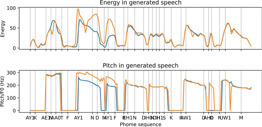
Instead of only using the SFVs as additional information
                                                                                 to the embedding, the third adaptation builds further upon the
                                                                                 previous introduced model in Sec V-B and also uses these
                                                                                 SFVs as additional input to their respective predictors. Hence,
                                                                                 the predictors also receive direct information of their respective
                                                                                 feature. This is done by appending them to the encoder output
                                                                                 to create a (2, #PHONEME) vector. This two dimensional
                                                                                 matrix is then used as input where the first convolutional layer
                                                                                 mixes the information.
                                                                                 Because of this, this model is refered to as ’epi’ which stands
                                                                                 for Embedding and Predictor Input.
                                                                                 D. Add pitch and energy to predictor output
Fig. 5. A (synthetic) example of an SFV to show the idea. Note how for the
last word, as it has a mapping from multiple words in the source, the average
is being taken

   For this adaptation a Source Feature Vector (SFV) is being
calculated and used to give the model information on the
source pitch and energy.
The first step in creating the SFVs is to calculate the average
pitch and energy for each word in the source speech. After-
wards with the help of multilingual alignment, where each
word of a source sentence is mapped to their corresponding
word in the translation, these SFVs can be mapped to the
target language. This way a vector is created where for each
phoneme in the target language either contains information on
                                                                                 Fig. 7. The addition exploitation where the pitch as energy SFV’s are summed
the average word-level value in the source language or, if it                    to the output of the predictors
was not alligned, a zero value. An example of an SFV can be
seen in Fig. 5                                                                      As the pitch and energy predictors try to do this on a
This model uses this additional energy and pitch information                     phoneme level, this can be exploited to influence the generated
by replacing the last 2 dimensions in the embedding layer by                     speech. As can be seen in Fig. 8 the energy and pitch in
the pitch and energy SFVs. This way the encoder takes the                        the generated speech can be changed by increasing the output
additional information from the SFVs as input which in turn                      values of their predictors before passing the values trough the
can help the variance adaptor to predict the pitch and energy.                   embedding. But in Fig 9 can be seen that increasing the pitch
In the results section this model will be called ’emb’ because                   and energy of words in the beginning of the sentence can
of the additional information in the embedding.                                  also change the pitch or energy at places where this might be
                                                                                 unwanted.
C. Word level pitch and energy as additional input to predictor                  In the fourth model, this is being exploited within the baseline
                                                                                 model by summing the SFV to the output of their respective
                                                                                 predictor. This way phonemes from words that have a below
                                                                                 average pitch or energy in the source language get their
                                                                                 predicted values lowered (because of having a negative z-score
                                                                                 added to them) and the same way words with an above average
                                                                                 value in the source language get their values increased in the
                                                                                 prediction.
                                                                                                     VI. E XPERIMENTAL SETUP
                                                                                 A. Preprocessing
                                                                                    To convert the transcript to a phoneme sequence and extract
                                                                                 the duration of each phoneme the Montreal Forced Alignment
                                                                                 tool [26] was used. The English sequences use the Arpabet
                                                                                 phoneme set and the German sequences use the prosodylab
                                                                                 format. To get the cross-lingual alignment the awesome-align
Fig. 6. the epi adaptation, the pitch and energy SFV’s are given as additional   [27] tool was used.
input to their respective predictors.                                            To train the model the audio data was resampled to 22050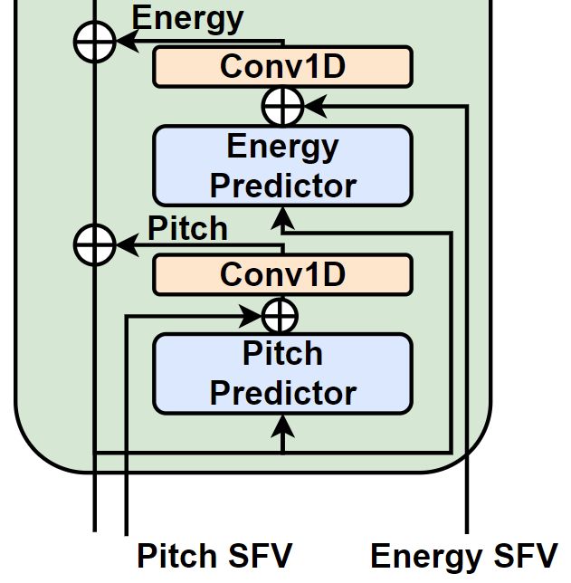
originating from the LibrivoxDeEn dataset but was realigned
using the same method described in Sec. IV.
C. Evaluation
To subjectively evaluate the speech quality a Mean Opinion
Score (MOS), where several native speakers are asked to
rate the naturalness of the generated speech between 0-5 (5
being the best), is approximated by using the deep learning
approach MOSNet [29]. To evaluate the training performance
of the models, the loss curves of the generated MFCC aswell
as the energy and pitch predictors on the validation set are
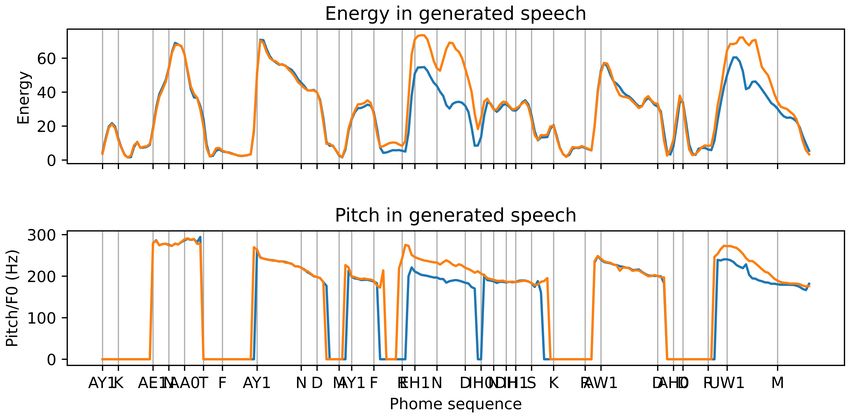
discussed. To evaluate the energy and pitch in the generated
speech, the same methods as in the FastSpeech2 [7] papers are
Fig. 8. input sentence: ”I cannot find my friend in this crowded room”, ”AY1
KAE1NAA0T FAY1ND MAY1 FREH1ND IH0N DHIH1S KRAW1DAH0D used. To evaluate the pitch the standard deviation, skewness
RUW1M” blue: using the output of the predictor, orange: increasing predicted and kurtosis for the pitch moments in the generated speech
energy and pitch at the phonemes corresponding to ”friend” and the first two is calculated [30], [31]. Ideally this would be as similar
to ”room”
as possible to our ground truth. Additionally the average
Dynamic Time Warping (DTW) distance of the pitch is also
computed with the help of the dtw-python package [32]. To
evaluate the energy the MAE compared to the ground truth is
being used. Similar to [7], the durations extracted by the MFA
are used in the length regulator to ensure the same generated
audio duration as the ground truth to calculate the MAE.
D. Hyperparameters
The hyperparameters for training can be seen in Tab. VI-D.
Further information on the number of hidden layers, embed-
TABLE II
H YPERPARAMETERS FOR TRAINING
Fig. 9. similar experimental setup as in Fig. 8 except this time the energy hyperparameter value
and pitch from the phonemes of ’find my’ are increased, initial learning rate 0.0001
end learning rate 0.00001
steps 100 000
batch size 6
kHz and the MFCC’s were extracted using a hop-size of 256,
a frame size of 1024 and a basis of 80. For training and testing
only audio files with a length between 1s and 20s were used. ding sizes, etc can be found in the GitHub repository [33].
VII. R ESULTS
B. Data size
A. Loss values
Some of the collected books either have bad microphone,
The loss curves for both the pitch and energy predictors,
need further processing to separate the speakers or do not have
and the generated MFCCs for the training and validation sets
enough samples to train a single speaker system. Therefore
are show in Fig. 10. For the training loss only the loss of the
in the continuation of this research the book Frankenstein by
baseline model is shown to make the graph visually clearer.
Mary Shelly4 is used. As a result there was only a total of 2335
The training losses of the adaptations are very similar (almost
audio files used for this research. 2 079 of these were used for
1:1) to this curve. Furthermore, it can also be seen that the
training, 129 for validation and 127 for testing. This number of
validation curves are very similar to each other. Additionally, it
samples for training is on the lower side compared to datasets
is clear that the pitch and energy predictors start to overfit after
usually used for single speaker TTS models such as LJSpeech
10 000 steps and stabilizes after this. The same can be said for
[28] where a total of 13,100 English audio fragments are used.
the validation loss on the predicted MFCCs, except here the
Nevertheless, it is still sufficient to train a TTS model but
convergence starts at 20 0000 steps. When training with dif-
might result in more/faster overfitting and worse audio quality.
ferent hyperparameters such as a bigger model, larger/smaller
The book used also had some misalignment on the source side
learning rates or a smaller/higher batch size similar results and
4 https://librivox.org/frankenstein-or-the-modern-prometheus-1818-by-
overfitting were achieved. Nevertheless, the best audio quality
mary-wollstonecraft-shelley/ and https://librivox.org/frankenstein-oder-der- was achieved with the model at 100k steps. For this reason
moderne-prometheus-by-mary-wollstonecraft-shelley/ further testing is done with the model achieved after 100 000Fig. 10. Train and validation losses. note: only the training losses for the baseline are reported as they are similar (almost 1:1) to the other models losses.
A step represents a pass of a single batch. Batches were shuffled during training.
TABLE III B. MOS estimation
L OSSES ON THE TEST SET FOR THE MODEL AFTER 20 K & 100 K TRAINING
STEPS . As mentioned in Sec. VI-C a Deep learning model has
NOTE : DURING TRAINING LOSSES ARE CALCULATED ON A BATCH SIZE OF been used to approximate the human MOS scores. Both the
6 BUT THIS TABLE WAS CALCULATED ON A BATCH SIZE OF 1 models after 20k and 100k training steps are evaluated on their
Pitch predictor Energy predictor generated speech.
Steps model MFCC loss
loss loss
baseline 0.692 0.254 0.346
TABLE IV
20k pho 0.667 0.270 0.345
MEAN MOS ESTIMATED BY MOSN ET ON THE T EST S ET
emb 0.731 0.254 0.345
epi 0.711 0.260 0.344 MOS at 20k MOS at 100k
gt 3.637 3.637
baseline 0.700 0.293 0.344 gt+MB-melGAN 3.679 3.679
100k pho 0.723 0.299 0.344
baseline 2.933 3.133
emb 0.726 0.290 0.347
pho 2.958 3.161
epi 0.755 0.290 0.344
emb 2.914 3.163
epi 2.933 3.159
addition 2.852 3.071
The first thing to note is that while the models after 20k
training steps on the initial hyperparameters but losses are also or 100k training steps have similar MFCC losses, all models
reported for the models at 20 000 steps. trained after 100k steps have a higher predicted MOS score
compared to the models at 20k training steps. Therefore these
Tab. III shows the losses of the pitch and energy predictors models will be considered as better since they are predicted
and the losses in the generated MFCCs on the test set. We to have a more natural speech and will be used for further
can see that all adaptations have a slightly lower loss than the evaluation.
baseline model on the generated MFCCs but perform similar Also can be seen that according to the predicted MOS scores
or worse on pitch and energy predictions. all adaptations have a slightly more natural audio quality
After 100k training steps this trend seems to be the same compared to the baseline, but the model only concatenating
where all models perform very similar to each other on the the SFV’s to the embedding has the highest score. The only
MFCC losses but seem to barely or not improve on the model that performs worse than the baseline is the exploitation
predicted pitch and energy. This indicates that adding the where the SFV’s get summed to the output of the predictors.
source information in different ways has limited to no impact
in increasing or decreasing the training losses. The impact on C. Pitch results
other characteristics such as the pitch, energy and the actual The pitch characteristics from the generated speech can be
generated speech are covered in the next subsections. found in Tab. V. Ideally these are as close as possible to the
Also note that no losses are reported for the exploitation of ground truth, represented by the pitch characteristics of our
the baseline model since as discussed in V-B it did not involve target speaker in the same test set, which are given in the
any training. first row. As can be seen, all trained model adaptations havean improvement on the baseline when looking at the standard TABLE VII
deviation (σ) and skewness (γ) but are lacking on the kurtosis SPEECH PITCH AND ENERGY METRICS WITH SFV VALUES BEING ZERO .
IMPROVEMENTS ON NON - ZERO SFV ARE SHOWN IN BOLD .
(κ). Noteably the model using the addition exploitation seems
to be the best at modeling the pitch characteristics of the GT σ γ κ dtw MAE MOS
speakers. emb zero sfv 40.187 -1.039 3.114 20.094 9.985 3.193
emb GT sfv 38.113 -1.000 3.104 20.329 10.002 3.163
epi zero sfv 38.988 -1.074 2.730 20.123 10.137 3.153
TABLE V epi GT sfv 38.704 -1.039 2.979 19.948 10.103 3.159
PITCH METRICS
σ γ κ DTW
GT 31.867 0.788 1.769 \ Tab. VII shows the achieved metrics when the SFV’s values
baseline 41.163 -1.138 2.627 21.423 are put to zero during inference. For the emb model, setting the
Pho 40.779 -1.063 2.931 19.876
emb 38.113 -1.000 3.104 20.329
SFV’s values to zero results in a better generated speech for
epi 38.704 -1.039 2.979 19.948 half of the metrics. While for the epi model, using zero-value
addition 42.174 -0.807 2.390 23.065 SFV’s results in worse values in five out of the six metrics used
for assessing the models. This indicates that using the SFV’s
When looking at the DTW distance the epi model (taking only within the embedding layer is possibly not benificial for
SFV as extra input in the predictors) has the lowest average this task as it results in worse performace in half of the mterics.
distance. The addition model, which has the most similar pitch But also adding the SFV’s as additional input to the predictors
characteristics, also has the highest DTW distance compared could be benificial as in this case using the GT SFV’s is still
to the other models. This could be because the pitch between better in five out of 6 metrics.
languages is not a one-to-one mapping and are therefore
summed on the wrong place or the predicted values become
too high or too low. VIII. D ISCUSSION
D. Energy results From the first experiment it can be seen that all models
are overfitting on the pitch and energy predictions. However,
To compare the energy in the generated speech the MAE
this does not seem to impact the actual performance of the
compared to the GT is computed. To ensure that the length
models in a negative way. This can be seen from the MOS
between the generated speech and the GT samples are the predictions when comparing the results achieved before and
same, the GT durations for each phoneme are used in the after overfitting on the training data. Also can be seen that
length regulator. From Tab. VI can be seen that when evalua- including or excluding source data during training does also
not result in more or less over fitting and suggests that this
TABLE VI
ENERGY MAE COMPARED TO GT
is mainly due to the low amount of data or the model’s
characteristics.
baseline pho emb epi addition Additionally, from the predicted MOS scores it can be seen
Energy
MAE
10.039 10.110 10.002 10.103 11.042 that including information from the source speaker can help
on improving the naturalness of the generated speech samples.
tion the energy, the emb model does slightly better compared Including source information can also help in improving the
to the baseline model. Generally all models have a similar modeling of the pitch characteristics of the generated speech
MAE except for the addition model which has the highest as most models improve over the baseline at modeling the
error. This indicates that using additional information from the standard deviation and skeweness of the pitch. Also the
source speaker did not help in improving much on the energy dynamic time warping distance from the generated speech
in the generated speech within the scope of this research. It compared to the ground truth is reduced by using additional
can also be seen again that adding the source energy could source information while training the model. When summing
result in a higher or lower estimate or at the wrong places the SFV’s to the predictions the DTW and standard deviation
again which in return results in a higher MAE. increase indicating that the pitch in the generated speech may
be becoming too high or is placed at the wrong places. This
E. Ablation study on the influence of SFV effect of the addition model can also be seen in Fig. 9 where
To have a closer look at the influence of the SFV on the the pitch is also being changed in places of the speech where
pitch and energy in the generated speech the SFV’s are set the predictor values were unchanged.
to zero before passing them trough the emb and epi model. At the energy level of the generated speech there is a slight
Afterwards the same metrics as the previous three sections improvement when adding the energy SFV to the embedding
are calculated. The values achieved with the SFV’s extracted dimension but the other models do not improve over the
from the source speech are also given as GT in the table, these baseline.
values are the same that are presented in earlier subsections. When doing and ablation study on the effect of the SFV’s
note: giving zero as value is the same as the mean value of on the model, conflicting results were seen where not using
the pitch or energy because of the z-score-normalization. any information from the source could result in better metrics.In a case where it would not be possible to extract the [5] M. Eck, I. Lane, Y. Zhang, and A. Waibel, “Jibbigo: Speech-to-
SFVs from the source audio it has been shown that using the speech translation on mobile devices,” in 2010 IEEE Spoken Language
Technology Workshop, 2010, pp. 165–166.
phoneme transcript from the source text can also be beneficial [6] W. D. Lewis, “Skype translator: Breaking down language and hearing
to increase the speech quality over the baseline. barriers,” Translating and the Computer (TC37), vol. 10, pp. 125–149,
Out of all these models it is hard to say wich approach is the 2015.
[7] Y. Ren, C. Hu, X. Tan, T. Qin, S. Zhao, Z. Zhao, and T.-Y. Liu,
best. Using the SFV’s only in the embedding seems to improve “Fastspeech 2: Fast and high-quality end-to-end text to speech,” 2021.
the most on almost all metrics compared to the baseline [8] Y. Ren, Y. Ruan, X. Tan, T. Qin, S. Zhao, Z. Zhao, and T.-Y. Liu,
method, but the ablation experiment gives conflicting results “Fastspeech: Fast, robust and controllable text to speech,” 2019.
and shows that there might be other reasons for this too. Also [9] MircosoftAzure, “Speech translation.” [Online]. Avail-
able: https://azure.microsoft.com/en-us/services/cognitive-services/
depending on the environment it might not always be possible speech-translation/#features
to create these SFV’s and then only using the phonemes, which [10] W. Wahlster, Verbmobil: Foundations of Speech-to-Speech Translation,
also improves over the baseline, as additional input could be ser. Artificial Intelligence. Springer Berlin Heidelberg, 2013. [Online].
Available: https://books.google.be/books?id=NoqrCAAAQBAJ
used. [11] Wolfgang. [Online]. Available: https://verbmobil.dfki.de/ww.html
[12] T. Do, T. Toda, G. Neubig, S. Sakti, and S. Nakamura, “Preserving word-
IX. C ONCLUSION level emphasis in speech-to-speech translation,” IEEE/ACM Transactions
on Audio, Speech, and Language Processing, vol. PP, pp. 1–1, 12 2016.
In this paper an effective way has been introduced to create
[13] R. Skerry-Ryan, E. Battenberg, Y. Xiao, Y. Wang, D. Stanton, J. Shor,
a bilingual speech parallel dataset with speech and translation R. J. Weiss, R. Clark, and R. A. Saurous, “Towards end-to-end prosody
quadruplets by building further upon already existing data. The transfer for expressive speech synthesis with tacotron,” 2018.
introduced method has multiple advantages and is shown to [14] Y. Wang, R. Skerry-Ryan, D. Stanton, Y. Wu, R. J. Weiss, N. Jaitly,
Z. Yang, Y. Xiao, Z. Chen, S. Bengio, Q. Le, Y. Agiomyrgiannakis,
be able to be used for a single-speaker TTS system. To use R. Clark, and R. A. Saurous, “Tacotron: Towards end-to-end speech
this method for a multi speaker TTS model further steps such synthesis,” 2017.
a speaker recognition are needed. [15] B. Beilharz, X. Sun, S. Karimova, and S. Riezler, “Librivoxdeen: A
corpus for german-to-english speech translation and speech recognition,”
Additionally, this dataset is used to incorporate additional Proceedings of the Language Resources and Evaluation Conference,
source information during training and inference of a Fast- 2020. [Online]. Available: https://arxiv.org/pdf/1910.07924.pdf
Speech 2 model in a Speech-To-Speech translation environ- [16] C. Wang, A. Wu, and J. Pino, “Covost 2 and massively multilingual
speech-to-text translation,” 2020.
ment. The trained models seem to mainly improve on having [17] R. Cattoni, M. A. Di Gangi, L. Bentivogli, M. Negri, and
a better pitch characteristic as the target and have a higher M. Turchi, “Must-c: A multilingual corpus for end-to-end speech
predicted MOS score by using additional information from the translation,” Computer Speech & Language, vol. 66, p. 101155, 2021.
[Online]. Available: https://www.sciencedirect.com/science/article/pii/
source audio. On the energy level of the generated speech the S0885230820300887
adaptations do not seem to benifit much from the additional [18] M. Post, G. Kumar, A. Lopez, D. Karakos, C. Callison-Burch, and
source inromation. For some of the addaptations conflicting S. Khudanpur, “Improved speech-to-text translation with the Fisher and
results are achieved in the ablation study and thus might need Callhome Spanish–English speech translation corpus,” in Proceedings of
the International Workshop on Spoken Language Translation (IWSLT),
further investigation. However, this is not the case for all Heidelberg, Germany, December 2013.
models presented in this work. [19] M. Sečujski, B. Gerazov, T. Csapó, V. Delić, P. Garner, A. Gjoreski,
D. Guennec, Z. Ivanovski, A. Melov, G. Németh, A. Stojkovikj, and
X. F UTURE W ORK G. Szaszák, “Design of a speech corpus for research on cross-lingual
prosody transfer,” 08 2016, pp. 199–206.
As future work in this research a model with more data [20] M. Kurimo, W. Byrne, J. Dines, P. N. Garner, M. Gibson, Y. Guan,
could be trained as this could result in less overfitting on the T. Hirsimäki, R. Karhila, S. King, H. Liang, K. Oura, L. Saheer,
M. Shannon, S. Shiota, and J. Tian, “Personalising speech-to-speech
training data and to further investigate the effect of the SFVs. translation in the EMIME project,” in Proceedings of the ACL
Additionally it would be interesting to look at the difference 2010 System Demonstrations. Uppsala, Sweden: Association for
between alligned and unalligned words and see if the SFVs Computational Linguistics, Jul. 2010, pp. 48–53. [Online]. Available:
https://www.aclweb.org/anthology/P10-4009
reduce the difference compared with the ground truth audio in [21] N. Rossenbach, A. Zeyer, R. Schlüter, and H. Ney, “Generating synthetic
the case where words are alligned or not. audio data for attention-based speech recognition systems,” 2020.
Since the proposed way to collect data can provide multiple- [22] J. Li, R. Gadde, B. Ginsburg, and V. Lavrukhin, “Training neural speech
to-one speaker and one-to-many speakers parallel sentences it recognition systems with synthetic speech augmentation,” 2018.
[23] J. Shen, R. Pang, R. J. Weiss, M. Schuster, N. Jaitly, Z. Yang, Z. Chen,
could also be interesting to see if the SFVs and their influence Y. Zhang, Y. Wang, R. Skerry-Ryan, R. A. Saurous, Y. Agiomyrgian-
is dependent on the source speaker or if it is not. And how the nakis, and Y. Wu, “Natural tts synthesis by conditioning wavenet on mel
source speaker could possible affect the generated speech. spectrogram predictions,” 2018.
[24] G. Yang, S. Yang, K. Liu, P. Fang, W. Chen, and L. Xie, “Multi-band
melgan: Faster waveform generation for high-quality text-to-speech,”
R EFERENCES 2020.
[1] W. J. Hutchins, The development and use of machine translation systems [25] A. Pettarin, “aeneas,” Mar 2017. [Online]. Available: https://www.
and computer-based translation tools. Bahri, 2003. readbeyond.it/aeneas/
[2] S. Nakamura, “Overcoming the language barrier with speech translation [26] M. McAuliffe, M. Socolof, S. Mihuc, M. Wagner, and M. Sonderegger,
technology,” Citeseer, Tech. Rep., 2009. “Montreal forced aligner: Trainable text-speech alignment using kaldi,”
[3] D. Bahdanau, K. Cho, and Y. Bengio, “Neural machine translation by in INTERSPEECH, 08 2017, pp. 498–502.
jointly learning to align and translate,” 2016. [27] Z.-Y. Dou and G. Neubig, “Word alignment by fine-tuning embeddings
[4] M. Sperber and M. Paulik, “Speech translation and the end-to-end on parallel corpora,” in Conference of the European Chapter of the
promise: Taking stock of where we are,” 2020. Association for Computational Linguistics (EACL), 2021.[28] K. Ito and L. Johnson, “The lj speech dataset,” https://keithito.com/
LJ-Speech-Dataset/, 2017.
[29] C. Lo, S. Fu, W. Huang, X. Wang, J. Yamagishi, Y. Tsao, and
H. Wang, “Mosnet: Deep learning based objective assessment for voice
conversion,” CoRR, vol. abs/1904.08352, 2019. [Online]. Available:
http://arxiv.org/abs/1904.08352
[30] O. Niebuhr and R. Skarnitzl, “Measuring a speaker’s acoustic correlates
of pitch -but which? a contrastive analysis based on perceived speaker
charisma,” 08 2019.
[31] B. Andreeva, G. Demenko, B. Möbius, F. Zimmerer, J. Jügler, and
M. Oleskowicz-Popiel, “Differences of pitch profiles in germanic and
slavic languages,” 09 2014.
[32] T. Giorgino, “Computing and visualizing dynamic time warping
alignments in r: The dtw package,” Journal of Statistical Software,
Articles, vol. 31, no. 7, pp. 1–24, 2009. [Online]. Available:
https://www.jstatsoft.org/v031/i07
[33] TensorSpeech, “Tensorspeech/tensorflowtts.” [Online]. Avail-
able: https://github.com/TensorSpeech/TensorFlowTTS/blob/master/
examples/fastspeech2/conf/fastspeech2.v2.yamlYou can also read