PASSIVE MICROWAVE SENSING
←
→
Page content transcription
If your browser does not render page correctly, please read the page content below
Philipson & Philpot: Remote Sensing Fundamentals Passive Microwave 1
W.D. Philpot, Cornell University, Fall 2012
10. PASSIVE MICROWAVE SENSING
10.1 Concepts of Microwave Radiometry
A microwave radiometer is a passive sensor that simply measures electromagnetic energy
radiated towards it from some target or area. As a passive sensor, it is related more to the classical
optical and IR sensors than to radar, its companion active microwave sensor. The energy detected
by a radiometer at microwave frequencies is the thermal emission from the target itself as well as
thermal emission from the sky that arrives at the radiometer after reflection from the target. The
thermal emission depends on the product of the target's absolute temperature and its emissivity, but
at microwave frequencies (in contrast to the thermal infrared) it is the change in emissivity rather
than the change in temperature that produces most of the significant differences between the various
targets. The intervening atmosphere between the target and the radiometer can have an adverse
effect on the measurement by attenuating the desired target signal and contributing unwanted
thermal radiated energy due to its own temperature and emissivity.
The microwave portion of the electromagnetic spectrum includes wavelengths from 0.1 mm to
more than 1 m. It is more common to refer to microwave radiation in terms of frequency, f, rather
than wavelength, . Recall that c = f, where c is the speed of light. In frequency then, the
microwave range is from 300 GHz to 0.3 GHz. Most radiometers operate in the range from 0.4-35
GHz (0.8-75 cm). Atmospheric attenuation of microwave radiation is primarily through absorption
by H20 and O2 and absorption is strongest at the shortest wavelength (Figure 10.1). Attenuation is
very low for > 3 cm (f < 10 GHz). In general µwave radiation is not greatly influenced by cloud
or fog, especially for > 3 cm.
Figure 10.1: Atmospheric absorption in the microwave region. Adapted from
http://www.rss.chalmers.se/rsg/Education/RSUM/Chap_A2002.PDF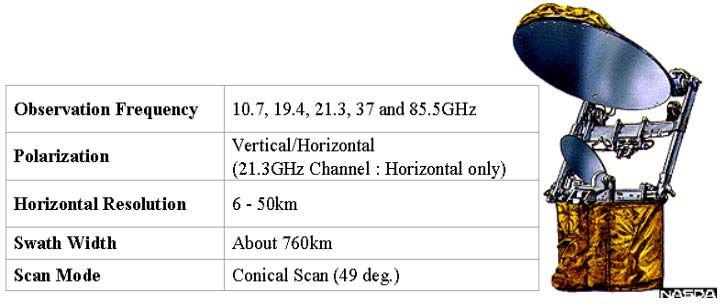
Philipson & Philpot: Remote Sensing Fundamentals Passive Microwave 2
W.D. Philpot, Cornell University, Fall 2012
Microwave sensing can be done day or night, in essentially any weather, particularly when
operated at frequencies less than 10 to 15 GHz. Note also that the atmosphere is essentially opaque
for f > 300 GHz ( < 1 mm).
10.2 Brightness temperature
The main parameter of interest being measured in microwave radiometry is the radiometric
temperature or brightness temperature of the source. The brightness temperature of an object is the
temperature of a blackbody with the same brightness (i.e., the same radiance) as the object sensed.
The most widely accepted terminology converts radiation received to an equivalent radiometric
(brightness) temperature in degrees Kelvin.
The maximum possible radiation that a body can emit at any given temperature, T, and
wavelength, , is described by Planck's Equation (see Chap. 3 of the monograph):
2hc 2
M (10.1)
hc
5 exp 1
kT
Using the Taylor series expansion we express the exponential term as:
2 3
c hc 1 hc 1 hc
exp 1 (10.2)
T kT 2! kT 3! kT
In the microwave region, since T >> hc/k, then all but the first two terms of the expansion may be
ignored and [exp(hc/kT) –1] hc/kT in Equation 10.1. With this approximation, the Planck's
equation reduces to the Rayleigh-Jeans approximation:
2ck
M 4 T (10.3)
where k is Boltzmann's constant. Thus, in the microwave region the radiation received from an
object is directly proportional to T. There is then a relatively small linear temperature dependence
compared with the fourth power of temperature dependence found in IR regions. This is apparent in
Figure 10.5 where emittance over a large range of earth temperatures varies by only a small fraction
of the change in emittance with wavelength. Note also that the emittance drops by more than two
orders of magnitude over the range of wavelengths typically used for passive microwave sensing,
highlighting one of the problems of sensing in this spectral region: the very low signal. The thermal
emittance from a body at typical earth temperatures is much less in the microwave than in the IR.
A direct consequence of the low signal is the relatively crude spatial resolution microwave
radiometers. In order to compensate for the low signal it is necessary to view a large area. In
addition, the resolution is partially a consequence of the antenna characteristics which will be dealt
with in a later section.
As with sensing in the thermal region, we must consider emissivity when dealing with real
sources:
M = Mbb = (2ck/4) Tbb (10.4)
Clearly, microwave radiation is proportionally more sensitive to emissivity variations than is
thermal infrared, and much of the observed variability will be due to differences in emissivity.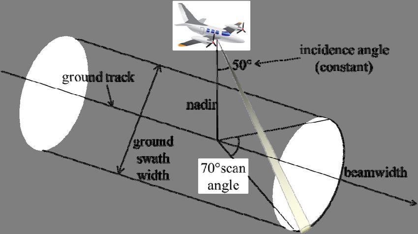
Philipson & Philpot: Remote Sensing Fundamentals Passive Microwave 3
W.D. Philpot, Cornell University, Fall 2012
The radiometric temperature of objects at the earth's surface is called the brightness temperature,
and is related to the true or thermometric temperature as:
TB = Tbb (10.5)
In the microwave region materials have large variations in emissivity, , which may vary from 0.41
for liquid water to almost 1.0 for ice; thus for a water surface with ice floating in it, the water
appears very cold and the ice very warm. Other materials have different emissivities, generally
between 0.4 and 1.0.
Figure 10.2: Variation in emittance with wavelength (frequency). The change with
temperature is relatively small.
Emissivity is a function of several variables including the dielectric properties of the material
(inherent conductivity, water content, and salinity), the viewing angle and polarization of the
detector, and the surface roughness of the emitting material. In the microwave range emissivity is
inversely proportional to the relative permittivity, r, which is a measure of a material’s ability to
transmit (or “permit”) an electric field, and consists of a real (scattering) component, ', and an
imaginary (absorption) component, ".
r = 'scattering + i"absorption (10.6)
The real part of the permittivity, the dielectric constant, ', is a measure of the ability of a
material to store a charge from an applied electromagnetic field and then transmit that energy. In
general, the greater the dielectric constant of a material, the slower microwave energy will move
through it and the lower the emissivity. Indeed, since the absorption term is generally negligible for
most environmental remote sensing applications it is reasonable to assume that the emissivity will
be inversely proportional to the dielectric constant, i.e., that:
1 / 'scattering (10.7)
For example, Most earth materials have a dielectric constant in the range of 1 to 4 (air=1, veg=3,
ice=3.2). Liquid water, on the other hand, is a polar molecule, is very responsive to an electric field
(conductive), and thus has a high dielectric constant ('water ~80), suggesting that moisture contentPhilipson & Philpot: Remote Sensing Fundamentals Passive Microwave 4
W.D. Philpot, Cornell University, Fall 2012
will lower the brightness temperature. Similarly, salinity will tend to increase the conductivity of
the soil, increase the dielectric constant, and thus decrease the emissivity.
10.3 Polarization
Polarization is an inherent characteristic of microwave sensors. This is convenient, since the
emissivity is also strongly dependent on polarization. Polarization for microwave sensing is
generally described as vertical or horizontal (rather than parallel or perpendicular). As illustrated in
Figure 10.3, vertical polarization is essentially equivalent to parallel polarization (the electric vector
is in the plane of the incident radiation and the normal to the target surface) and horizontal
polarization is basically equivalent to perpendicular polarization.
Figure 10.3: Diagram illustrating the orientation of polarization for microwave sensing.
Figure 10.4: Sensitivity of emissivity to polarization. From: Microwave Resources,
Sec.8.6:Polarization of Earth-Atmosphere Emitted Energy.
http://www.meted.ucar.edu/npoess/microwave_topics/resources/print.htm#s8p1.
Emissivity varies with polarization. This is particularly true when moisture content is a
consideration, but is also an issue even in dry a conditions. As is illustrated in Figure 10.4,
emissivity varies both with polarization and frequency. It also varies with look angle, further
complicating the problem.Philipson & Philpot: Remote Sensing Fundamentals Passive Microwave 5
W.D. Philpot, Cornell University, Fall 2012
10.4 Influence of the atmosphere and active sources
10.4.1 Observed brightness temperature from a reflecting surface.
A µ-wave radiometric sensor (radiometer or scanning radiometer) is a temperature measuring
device; its output is calibrated in °K. For a microwave sensor near a target, the observed brightness
temperature, TB, is the sum of radiation received directly from the target source, plus the sky
radiation reflected by the source (Figure 10.5).
Figure 10.5: A microwave sensor sees emission from the target as well as from reflected
skylight.
If the surface of an object is very smooth it can also reflect radiation from the sky and from
space. Thus smooth water will reflect the sky temperature and the remotely observed temperature
will depend on the reflected energy of the surface and on the polarization of the radiation as well as
on the temperature and emissivity. Water, if it is smooth, will reflect the very low sky temperature.
However, if it is choppy the reflectivity and emissivity are changed and the apparent temperature
can increase considerably. That is, for an opaque surface,
TB = Ts + Ti(i) = Ts + (1–)Ti(i) (10.8)
where we have dropped the subscript, , indicating an average emissivity and reflectance. There are
several points worth noting:
The observed brightness of objects with high (1) is little influenced by other sources
of moderate brightness temperature.
The observed brightness of objects with high reflectivity (low ) is much affected by the
background radiation.
Natural materials may have relatively low emissivities in the µ-wave region. For
example, in the infrared, = 0.8 to 0.9+; in the µ-wave, =0.6 to 0.9
w for water < 0.5; ice 1;
ocean 0.4; earth > 0.85
Emissivity is a function of angle of incidence () and azimuth (), as well as polarization:
v(,) or H(,). It is generally found that as the angle increase a drop in apparent
temperature is due principally to the non-Lambertian quality of the emitter. In some
cases, however, a rise in apparent temperature is found as the angle is increased.
Another effect is the polarization of the radiation detected. It has been found that
significant differences exist in emission when observed in vertical and horizontal
polarization. Note: Blackbody radiation is randomly polarized -- radiation from real
bodies may not be.Philipson & Philpot: Remote Sensing Fundamentals Passive Microwave 6
W.D. Philpot, Cornell University, Fall 2012
Emissivities are determined by surface properties (roughness) and, to some extent, by
subsurface properties (dielectric coefficient or, more properly, "complex dielectric
coefficient").
Note that dielectric properties vary with , water content, salinity, etc.
If the reflecting surface is rough compared to – i.e., a partially diffuse surface – then
interference (external) sources at other incidence angles may contribute to brightness
observed; will also vary.
10.4.2 Brightness observed through an absorbing medium (atmosphere)
One remaining factor in microwave radiometry, as in all airborne or satellite sensors, is
atmospheric absorption, re-emission, and scattering. For wavelengths longer than 3 cm the air is
quite clear; however, shorter than this there is significant absorption by H2O and O2 components.
Such gases also re-emit radiation at similar frequencies thus making interpretation even more
difficult. This fact can, however, be used to advantage if it is the component of the atmosphere that
the observer wishes to see.
Consider the situation for which a microwave sensor is viewing the earth through the
absorbing medium of the atmosphere. Recalling Kirchoff's Law: = + + = 1, and recognizing
that reflectance by the atmosphere is near zero in the microwave, we may write:
a = 1 - a = a (10.9)
where the subscript indicates that the quantities refer to the atmosphere. Assuming thermal
equilibrium, then atmospheric absorption and emissivity are equivalent and we have:
aTa = aTa, (10.10)
where Ta is the atmospheric temperature. The brightness temperature of a surface viewed through
an absorbing medium is then described by:
TB Ts
1 a Ta (10.11)
a
attenuated energy absorbed
brightness and reradiated
temperature by the medium
of the surface in the optical path
If we also consider radiation reflected by the surface from external sources (e.g., clouds) then we
have the more complex situation illustrated in Figure 10.6. The observed brightness temperature
will then be given by:
TB { [ Ti i (1 i )Ta1 εTs } s +
]ρ+ (1+i ) Ta2 (10.12)
External energy External energy Energy Energy absorbed
which is not absorbed, which is absorbed emitted and re-radiated by
i.e., it reaches the and re-emitted by by the the atmosphere
earth's surface the atmosphere surface at at temperature Ta2
at temperature Ti at temperature Ta1 temp. TsPhilipson & Philpot: Remote Sensing Fundamentals Passive Microwave 7
W.D. Philpot, Cornell University, Fall 2012
Figure 10.6: Combined influence of active (external) sources and atmosphere
Ti = brightness temperature from external sources.
1 = transmittance of the whole atmosphere in direction .
2 = transmittance of atmosphere between surface and sensor.
Ta1 = mean temperature of whole atmosphere.
Ta2 = mean temperature of atmosphere between surface and sensor.
10.4.3 Summary
The radiation collected appears is treated as an equivalent temperature, that is, the temperature
of a blackbody source which would produce the same radiation in the bandwidth of the system. The
equivalent temperature is determined by comparing the level at the antenna with that of a reference
resistance held at a constant temperature. Comparison is carried out by rapidly switching from one
to the other and measuring signal difference.
This equivalent temperature which is recorded is not equal to the temperature of the area
observed. Since it is a passive system a large number of factors contribute to the radiation levels
thus complicating interpretation. Some of these factors are:
1.actual temperature of sources.
2.emissivities (function of surface, subsurface, dielectric properties, etc.)
3.observation angle and direction (also angle of incident radiation.
4.wavelength, ( or frequency, f)
5.polarization (blackbody radiation is randomly polarized; consider object & reflected)
6.external sources, atmospheric interactions, sky reflections, etc.
7.noise from the radiometer itself.
10.5 Antennas
10.5.1 Antennas and radiometric measurements
The detector for microwave radiation is an antenna. The apparent temperature observed at the
antenna -- the antenna temperature -- is related to the brightness temperature, TB, by:
TA
T
B G d d (10.13)
where is the IFOV of the system and G is the antenna gain. This equation basically states that the
apparent temperature at the antenna is a function of the viewing angle (beamwidth) and wavelength
range (bandwidth) of the antenna.
The beamwidth is defined as the angular interval over which the antenna's power pattern exceeds
one-half of its maximum value ("half-power" beamwidth). A typical microwave radio-meter has aPhilipson & Philpot: Remote Sensing Fundamentals Passive Microwave 8
W.D. Philpot, Cornell University, Fall 2012
pencil-beam antenna with high sensitivity within a small solid angle. The sensitivity of the antenna
is highly directional and defines the angular (or spatial) resolution of the system.
Antennas, like lenses, are diffraction limited. As such, the angular resolution of a diffraction
limited system will be on the order of /d, where d is the size of the aperture (i.e., length or
diameter). In the optical range (UV/VNIR/SWIR), where the /d ratio is on the order of 10-5,
diffraction effects exist but are relatively subtle. However, the ratio in the microwave is on the
order of 10-1 and the diffraction effects are much more significant. In the optical domain, diffraction
effects can be seen if a plane wave is incident on a narrow slit (Figure 10.7). The resulting intensity
(diffraction) pattern on a screen parallel to the slit plate is a diffraction pattern evidence of the
wave nature of light. As the slit width increases the side lobes decrease in amplitude and occur
closer to the center lobe. In an optical system this corresponds to an increase in the angular
resolution as the diameter of the lens (or aperture) increases.
Figure 10.7: Single thin slit diffraction pattern.
In microwave systems, where the aperture size is on the same order as the wavelength being
sensed, the magnitude of the side lobes is frequently significant and troublesome (Figure 10.8). Part
of the design criterion for antennae is the minimization of the side lobes, particularly when a highly
directional beam is needed.
Figure 10.8: Typical antenna power pattern in polar coordinates.
10.5.2 Simple dipole antennas
Since the antenna is the critical detection device for both passive and active (radar) systems, it
is worth spending some effort learning a few basics of antenna design. To begin, consider a simple
dipole antenna. Although this is probably the simplest of all antennas, it forms the core of many
more sophisticated antennas. This is the type of antenna commonly used for a car radio and for FM
radio. The dipole is so named because it has two electrical poles, not two physical poles (it also has
two zeros and could have been called a di-zero antenna). When the length is such that the poles are
at ends of the conductor and the zeros are at the center, the antenna will be exactly /2 long, where
is the wavelength of the radiation, and it will be an efficient radiatorPhilipson & Philpot: Remote Sensing Fundamentals Thermal Sensing 10.9
W.D. Philpot, Cornell University, Fall 2012
a)
b)
Figure 10.9: Simple dipole antenna. The optimal size of the antenna is /2.
A dipole can be fed anywhere along its length, however center fed (your FM radio antenna)
and end fed (your car antenna) are the most common. When fed at the center, it presents a pure
resistive, balanced resistance to the feed line. If the antenna is oriented vertically, then vertically
polarized radiation from all (2π) directions in the horizontal plane will induce a current in the
antenna (Figure 10.9a). The corresponding directional sensitivity of the dipole antenna is shown in
Figure 10.9b. The antenna's directionality is related to its polarization. It will not respond to
radiation arriving along the axis of the antenna and will respond most effectively to vertically
polarized radiation incident at 90 from the antenna axis. This polarization sensitivity is
characteristic of all microwave system since polarization is an inherent property of the microwave
detector.
A simple dipole antenna has many uses, but remote sensing is not one of them. For remote
sensing from aircraft and satellite (as well as for many other purposes) it is essential to be able to
select the direction from which the radiation is coming. The simplest way to improve the
directionality of the antenna is to place a reflector behind the primary antenna (Figure 10.10a). A
reflector is often a flat, perforated plate. It will essentially limit the sensitivity of the detector to one
hemisphere. A similar idea is to add passive elements in front of the antenna (directors). Directors
alter the directivity of the antenna so that the gain is improved in front of the dipole. Most antennas
have more than one director, and the more directors the antenna has the smaller the beamwidth.
a. b.
Figure 10.10: Directional response of dipole antennas with passive focusing elements.
a. Dipole antenna with a reflector.
b. Dipole antenna with a directors and a reflector.Philipson & Philpot: Remote Sensing Fundamentals Thermal Sensing 10.10
W.D. Philpot, Cornell University, Fall 2012
10.5.3 Parabolic dish antennas
Taking the idea of the reflector one step farther, one may put the dipole antenna at the focus of
a parabolic dish (Figure 10.11a). In this case, the larger the antenna, the more narrow the major
lobe will be, and the beamwidth will be ~ /d where d is the diameter of the dish. Note that the
antenna is still only sensitive to radiation polarized along the axis of the dipole antenna at the focus.
Figure 10.11: Dish antenna with a dipole receiver.
a. Receiving geometry of the dish antenna.
b. Directional response of the dish antenna.
Note that the parabolic dish is merely collecting the radiation and redirecting it to the dipole
antenna which is the detecting element. The dish is the analog of a mirror or lens in an optical
system. Use of a horn, rather than a dipole antenna, at the focal point of the dish minimizes the loss
of energy (leakage) around the edges of the dish reflector and improves the overall gain of the
system.
There are several possible approaches for improving the sensitivity of microwave radiometers:
1) increase the beamwidth to collect more radiation spatially, 2) increase the bandwidth to collect
more radiation spectrally, or 3) integrate over long periods. Increasing the beamwidth is the most
common option for microwave radiometers. (The spot size of a typical satellite microwave
radiometer is many kilometers.) Increasing bandwidth may be effective for some applications, but
is often not a realistic option. Integrating over longer periods is only an option for systems that can
stare in one direction for an extended time. This can work for ground-based systems but is not very
worthwhile for use in aircraft or satellite.
10.5.4 Phased array antennas
Whenever two or more simple antenna elements (e.g. dipoles) are brought together and driven
from a source of power at the same frequency, the resulting antenna pattern becomes more complex
due to interference between the signals detected separately from each of the individual elements. At
some points, this interference may be constructive causing the transmitted signal to be increased.
At other points, the interference may be destructive causing a decrease or even a cancellation of
transmitted energy in that direction.
Focusing improves with the addition of more antenna elements. For example, four dipole
antennas placed near each other and monitored by a receiver set to receive in-phase signals results
in a narrower pattern than that for the 2-dipole case (Figure 10.12a). Of course, side lobes also
appear in the total antenna pattern. These are a characteristic, undesirable feature of most complex
antenna arrays. It is theoretically possible to suppress side lobes completely in an array of antenna
elements if the excitation of each element is controllable. The process of shaping the antenna
pattern so as to eliminate side lobes is called tapering. Eliminating side lobes results in less total
gain at the pattern maximum, however, and it yields a broader main lobe.Philipson & Philpot: Remote Sensing Fundamentals Thermal Sensing 10.11
W.D. Philpot, Cornell University, Fall 2012
Figure 10.12: Phased array antennas are used for focusing and pointing the antenna.
[Adapted from: http://www.haarp.alaska.edu/haarp/ant3.html ]
a. 4-element phased array with all antenna elements in phase.
b. 4-element phased array with a phase shift between the antenna
elements.
The angle at which the pattern maximum occurs can be changed by adjusting the phase of the
signals received from each of the antenna elements. With all elements in-phase, the pattern
maximum will occur perpendicular to the front of the array. By adjusting the relative phase, the
peak of the main lobe can be shifted (or steered) to a new angle relative to the array face (T4 in
Figure 10.12b). In general, the maximum signal strength at the new pointing angle is close to but
less than the perpendicular case.
When the pattern is steered to a new direction, the shape and direction of any side lobes that
may have originally been present changes. If the pattern is steered too far relative to the element
spacing, a new lobe (called a grating lobe) will appear with a peak in its pattern nearly equal to the
main lobe. The point where this occurs is the maximum useful steering angle.
10.5.5 Examples of specific systems
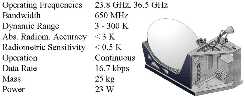
10.5.5.1 The RA-2 Microwave Radiometer (MWR)
The RA-2 Microwave Radiometer (MWR) is one of the instruments being flown on Envisat
(Launched March, 2002). The main objective of the MWR is the measurement of the integrated
atmospheric water vapor column and cloud liquid water content to provide correction terms for the
radar altimeter also flying on Envisat. In addition, MWR measurement data are useful for the
determination of surface emissivity and soil moisture over land, for surface energy budget
investigations to support atmospheric studies, and for ice characterization.
Figure 10.13: RA-2 Microwave Radiometer (MWR)Philipson & Philpot: Remote Sensing Fundamentals Thermal Sensing 10.12
W.D. Philpot, Cornell University, Fall 2012
10.5.5.2 Tropical Rainfall Measurement Mission (TRMM) Microwave Imager (TMI)
The TMI is a multi-channel/dual-polarized microwave radiometer which provides data related to
rainfall rates over the oceans. The TMI data are intended to be used together with the Precipitation
Radar (also flown on TRMM).
Figure 10.14: TRMM Microwave Imager (TMI)
10.5.5.3 Advanced Microwave Scanning Radiometer (AMSR-E)
This instrument has 12 channels at 6 frequencies. Horizontally and
vertically polarized radiation are measures separately at each frequency:
(6.925 GHz (56 km); 10.65 GHz (38 km); 18.7 GHz (21 km); 23.8 GHz (24
km); 36.5 GHz (24 km); 89.0 GHz (12 km). The AMSR-E, flying on the
EOS AQUA satellite, measures geophysical parameters supporting several
global change science and monitoring efforts, including precipitation,
oceanic water vapor, cloud water, near-surface wind speed, sea surface
temperature, soil moisture, snow cover, and sea ice parameters. All of these
measurements are critical to understanding the Earth's climate.
10.5.5.4 NASA's Passive Microwave Imaging System (PMIS)
(Description from NASA's Earth Observations Aircraft Remote Sensing Handbook, 1972, p 5 -54
to 5-56 and p. 6-60).
Although this is a very old system, and no longer in use, it provides a good example of a phased
array system. The 10.69-GHz passive microwave imaging system (PMIS) gathered low dimensional
quantitative antenna brightness temperature data over a variety of targets. The system was
composed of two airborne subsystem (described below) and a ground data system.
The PMIS consists two major subsystems. The first subsystem, the imaging radiometer, includes
the radiometer, antenna, and the radiometers mounted aboard the aircraft. The primary data outputs
are interfaced with an encoder which generates digital data for tape recordings. The second
subsystem, the airborne control and display, controls and monitors the imaging radiometer
subsystem and includes a switchable real-time readout for monitoring the instrument and
engineering outputs. A near real-time black-and-white image display provides a quick-look
capability. A camera records data from a second display.
Coverage: The antenna is a two-dimensional phrased array, electrically stepped to achieve scanning
transverse to the flight-path. the antenna scans along a cone which makes a 50° incidence anglePhilipson & Philpot: Remote Sensing Fundamentals Thermal Sensing 10.13
W.D. Philpot, Cornell University, Fall 2012
with the ground. A single antenna scan traces an arc on the ground forward of aircraft nadir (Figure
5-21). the antenna is dual polarized with two output ports. One for vertical polarization and the
other for horizontal polarization.
Operational capabilities: Predelivery specifications for the antenna are listed below; actual
operating values may differ.
System specifications: The specifications below apply to total system accuracy, including the
radome and antenna:
Frequency: 10.69-GHz (±5 MHz)
Bandwidth: 150 MHz (3 dB points)
Sensitivity: T rms for a V/h of 0.02 is less than 0.5° K
T rms for a V/h of 0.134 is less than 2.0° K
Absolute Accuracy: Less than 1.5° K
Antenna specifications:
Voltage standing wave ratio (VSWR): the input VSWR of the antenna system is less than 1.15
over the RF bandwidth.
Loss: dissipative loss of the antenna up to the antenna attachment reference
flange is 2 dB or less for all beam positions.
Coupling: the two output ports have minimum 20-dB isolation.
Polarization: linear for both vertical and horizonal axes.
Beamwidth: less than or equal to 1.8 ° (= ±0.25°) increasing the 2.7° at the scan
limits; constant 3° or less beam in the alongtrack direction (all nominal
between 3-dB points) measured to ±0.25°.
Beam efficiency: 90% or greater measured to ±1 percent.
Side lobes: less than -21 dB for any beam position throughout the scan.
Scan specification: scan angle:±35° transverse to the flight line; results in 44 scan positions.
Scan steps: produces a 20- to 30- percent overlap of adjacent beams (at their 3-dB
points); controls available to stop the beam scan on any beam position and
to manually step through all positions.
Scan rate: step controlled with 95 discrete rates; inputs for the stepped control are
from the Airborne Control and Display Sub-system. A manual override
permits the operator to independently insert ground speed in knots and
altitude vales in hundreds of feet.
Data Analysis: The PMIS data preprocessing is performed on the ground data station [Passive
Microwave Imaging System (PMIS) Microwave/Multispectral Data analysis Station (M/MDAS)].
The PMIS M/MDAS is a high-resolution color imaging and recording system. It is used for the
processing imaging, and recording (digital and film) of the 10.69 GHz passive microwave
radiometric data acquired by the PMIS imaging radiometer system.Philipson & Philpot: Remote Sensing Fundamentals Thermal Sensing 10.14 W.D. Philpot, Cornell University, Fall 2012 References: MacDowall, J. and B. H. Nodwell (1971) Resource satellites and remote airborne sensing for Canada. report No. 14: Remote-sensing devices. Dept. Energy, Mines & Resources, Ottawa, Canada. 125pp. National Academy of Sciences (1977) Earth resources sensing with microwave radiometry. In: Microwave remote sensing from space for earth resources surveys, Chapter 3. RC/CORSPERS- 77/1.
You can also read