Self-Optimizing Grinding Machines using Gaussian Process Models and Constrained Bayesian Optimization
←
→
Page content transcription
If your browser does not render page correctly, please read the page content below
1

                                           Self-Optimizing Grinding Machines using Gaussian Process Models
                                                         and Constrained Bayesian Optimization
                                                                    Markus Maier1 , Alisa Rupenyan1,2 , Christian Bobst3 and Konrad Wegener4

                                                                                                                    Abstract
                                                    In this study, self-optimization of a grinding machine is demonstrated with respect to production costs, while fulfilling quality
                                                and safety constraints. The quality requirements of the final workpiece are defined with respect to grinding burn and surface
                                                roughness, and the safety constrains are defined with respect to the temperature at the grinding surface. Grinding temperature is
                                                measured at the contact zone between grinding wheel and workpiece using a pyrometer and an optical fiber, which is embedded
                                                inside the rotating grinding wheel. Constrained Bayesian optimization combined with Gaussian process models is applied to
                                                determine the optimal feed rate and cutting speed of a cup wheel grinding machine manufacturing tungsten carbide cutting
arXiv:2006.05360v1 [eess.SY] 9 Jun 2020

                                                inserts. The approach results in the determination of optimal parameters for unknown workpiece and tool combinations after
                                                only a few grinding trials. It also incorporates the uncertainty of the constraints in the prediction of optimal parameters by using
                                                stochastic process models1 .

                                                                                                             I. I NTRODUCTION
                                             The selection of optimal grinding parameters is an important task because grinding is often one of the last manufacturing
                                          steps where failures lead to high financial losses. Today parameter selection is mainly performed by experienced operators
                                          using a trial and error approach. Self-optimization of grinding machines has been the subject of extensive research in industry
                                          and academia. The main challenge in grinding process optimization arises from the non-linear, stochastic and transient process
                                          properties. Already in 1994, Rowe et al. [1] reviewed artificial intelligence systems applied to grinding and listed various
                                          approaches such as knowledge-based systems, expert systems, fuzzy logic systems, neural net systems, and adaptive control
                                          optimization techniques. Over time, various models have been proposed to control specific grinding tasks. For example, in [2]
                                          a state-space model for the prediction of part size and surface roughness in cylindrical grinding is proposed and [3] reports an
                                          adaptive grinding force control. Modelling is strongly coupled with optimization. An overview on grinding process modelling
                                          and optimization is given in [4]. For example, in [5] a method for the optimization of a grinding process in batch production
                                          using a grinding process model and a dynamic programming approach to update process parameters between grinding cycles
                                          is demonstrated. In [6] constrained multi-objective optimization of grinding with Pareto fronts using genetic algorithms is
                                          shown. Another ingredient for optimization is process monitoring using measurements from force or power sensors, acoustic
                                          emission sensors and temperature sensors [7]. The combination of models, optimization techniques, sensor data, and material
                                          data enables intelligent, data-driven methods for process control and assistance, as demonstrated in [8]–[10]. In [8] the grinding
                                          cycles are adaptively optimized and grinding burn is prevented, [9] presents empirical models fitted with experimental data, used
                                          to find optimal process parameters based on optimization objective minimization subjected to constraints, and [10] describes
                                          a model-based assistant system for precision, productivity, and stability increase of centerless grinding.
                                             Current state of the art methods work well for specific tasks and niche applications where extensive training data is available
                                          or low model complexity is sufficient. However, industrial applications for general process optimization in grinding are still
                                          missing. Grinding processes are very sensitive to environmental conditions, and optimizing a grinding process on one machine
                                          does not necessarily result in the same performance on a different machine of the same type. Another obstacle is the lack of
                                          information such as physical properties of the grinding wheel and the workpiece because they are trade secrets of the respective
                                          manufacturer. Therefore, on-machine experiments are needed for optimization such as done today by experienced operators.
                                          Experimental design methods, such as the Taguchi method, can be used to determine on-machine experiments, as presented in
                                          [11]. The disadvantage of the Taguchi method is that knowledge gained during testing is not incorporated in the optimization.
                                             In the present study, Gaussian process (GP) regression is used for process modelling. Gaussian process regression is a
                                          powerful stochastic model, which is used widely to provide uncertainty estimation when dealing with stochastic data [12]. The
                                          main advantage of a Gaussian process regression is its flexibility, the in-built uncertainty prediction, and the non-parametric
                                          nature of the model. A detailed introduction to Gaussian process regression can be found in [12]. Based on a Gaussian
                                          process prior and available measurements, Gaussian process regression can be used to predict the mean and the variance for
                                          every arbitrary combination of input parameters. The estimated variance is useful to incorporate uncertainty in the process
                                          optimization based on the predictions from the Gaussian process regression.
                                            1  The authors are with Inspire AG, Zurich, Switzerland. {maier,rupenyan}@inspire.ethz.ch
                                            2 The author is with the Automatic Control Laboratory, Department of Electrical Engineering and Information Technology, ETH Zurich, Switzerland.
                                            3 The author is with Agathon AG, Bellach, Switzerland. christian.bobst@agathon.ch
                                            4 The author is with Institute for Machine Tools, Department of Mechanical and Process Engineering, ETH Zurich, Switzerland.
                                          wegener@iwf.mavt.ethz.ch
                                            1 This is a pre-print of an article published in The International Journal of Advanced Manufacturing Technology. The final authenticated version is available
                                          online with a DOI 10.1007/s00170-020-05369-9.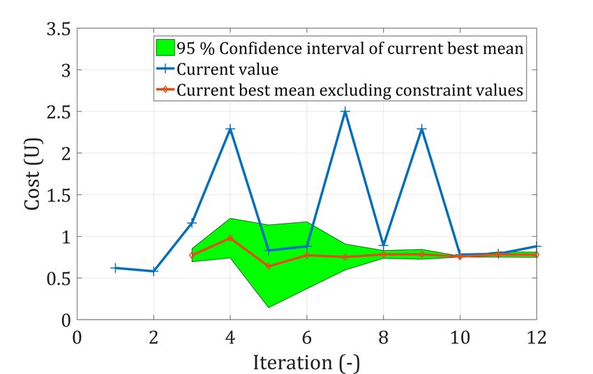
2
Gaussian process regression is used in combination with Bayesian optimization (BO), where it provides a surrogate model for
the unknown objective function. Bayesian optimization is a sequential design strategy for global optimization of an unknown
objective function, which is expensive to evaluate [13]. Bayesian optimization uses the predicted mean and variance functions of
the Gaussian process model of the objective to determine the next experimental point with high information content, afterwards
the GP model is updated with the newly available data [13]. This procedure is repeated until suitable process parameters are
found. Bayesian optimization has been successfully applied in hyperparameter tuning of learning algorithms [14], photovoltaic
power plants [15], and robotics [16]. Recently, it has also been successfully applied to the optimization of turning processes
[17], [18].
In this study, an autonomous process set-up is proposed where the cutting speed and the feed rate in grinding are opti-
mized based on combined measurements of roughness, temperature, and maximum dressing intervals. Constrained Bayesian
optimization is applied to enforce quality and safety constraints. This paper is organized as follows: A short introduction
to Bayesian optimization and Gaussian process models is provided first, followed by a methodology section explaining the
optimization objective, experimental set-up, and algorithm implementation. Afterwards, optimization results performed on a
cup wheel grinding process are reported and discussed.
II. BAYESIAN OPTIMIZATION AND G AUSSIAN PROCESS MODELS
A general introduction to Gaussian process models is given in [12] and an introduction to Bayesian optimization can be found
in [13]. According to [12], a Gaussian process represents a distribution over functions and is a collection of random variables,
which have a joint Gaussian distribution. A Gaussian process is fully defined by a mean function m(x) and a covariance
function k(x, x0 ) often referred as the kernel. In this study, a Matern 5 kernel with automatic relevance determination (ARD)
[12] is used,
√ √
5
k(x, x0 ) = σf2 1 + 5r + r2 exp − 5r) (1)
3
q
r = (x − x0 )T P−1 (x − x0 ) (2)
P = diag(l12 , l22 , ..., lD
2
) (3)
where σf2 is the signal variance, r is the distance between the input data points x and x0 (in this case, the input data are
process parameters that have to be optimized), and P is a diagonal matrix containing characteristic length scale parameters li2
for each input space dimension up to dimension D. The kernel function specifies the relation between the function values at
process parameters x and x0 , where for a short distance between the process parameters the corresponding function values are
similar whereas for larger distances higher variations are observed.
A Gaussian process is used as a prior for Gaussian process regression. In this study, the Gaussian process prior mean
function m(x) is assumed zero, specifying no expert knowledge. The resulting posterior mean µt and variance σt2 of the
Gaussian process regression at an arbitrary location x can be calculated as follows [12],
µt (x) = kT (x)(K + σN
2
I)−1 yt (4)
σt2 (x) = k(x, x) − kT (x)(K + σN
2
I)−1 k(x) (5)
k(x1 , x1 ) · · · k(x1 , xt )
K=
.. .. ..
(6)
. . .
k(xt , x1 ) · · · k(xt , xt )
2
where xt and yt are the vectors containing t pairs of measurements assumed to be corrupted with Gaussian noise N (0, σN ),
I is the identity matrix, K is the covariance matrix, and k(x) is a covariance vector between x and x1 to xt .
The length scales li2 in eq. (3), the signal variance σf2 in eq. (1), and the signal noise σN
2
in eq. (4) and eq. (5) are
hyperparameters of the Gaussian processes regression, which can be summarized in a hyperparameter vector θ. It is possible
to specify these hyperparameters before the Gaussian process regression based on expert knowledge. Another method, as
described in [12], is to determine the hyperparameters θ∗ based on available measurements by maximization of the marginal
log likelihood p(yt |θ).
1 1 t
log p(yt |θ) = − ytT (Kθ + σN
2
I)−1 yt − log |Kθ + σN
2
I| − log 2π (7)
2 2 2
θ∗ = argmax log p(yt |θ) (8)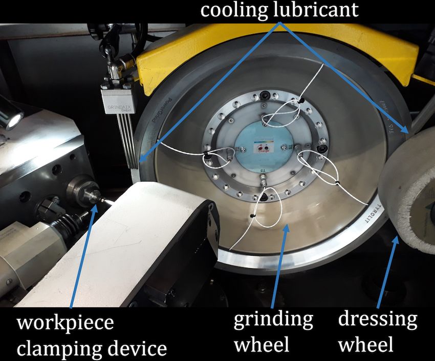
3

Fig. 1: Gaussian process regression for different hyperparameters. Panel (a): hyperparameters determined by maximizing the
marginal log likelihood using equation (8). Panel (b): results for high signal noise. Panel (c): results for short length scale
parameter. Panel (d): results for long length scale parameter.

A θ subscript is added to the covariance matrix in equation (7) to explicitly show its dependence on the hyperparameters
θ. Figure 1 shows the Gaussian process regression results exemplarily for different hyperparameters. In the example the
true cost function is set to y = (x − 0.2)2 and displayed for illustration (dotted black line). The true cost function was
evaluated at several process parameter values. The measurements are noisy observations of the true function ȳ = y + , where
 ∼ N (0, 5e − 4). These measurements are the input data points to the Gaussian process regression. Figure 1(a) shows the
Gaussian process regression for the hyperparameters maximizing the marginal log likelihood using equation (8). It can be
seen that with these hyperparameters the fit of the data is very good. A GP regression using the same data points but a high
signal noise hyperparameter is shown in Figure 1(b). The prediction of the true cost function is still reasonable but shows a
high overall uncertainty. Figure 1(c) shows the Gaussian process regression for a low length scale hyperparameter. In this case
more complex functions are also plausible candidates, which leads to high uncertainties between the measurements, where data
is missing. On the other hand on Figure 1(d) a Gaussian process regression for a very long length scale hyperparameter is
shown. In this case the generalization from the observed measurements results in a simple (nearly linear) function for the mean
function of the Gaussian process and in low uncertainty over the whole range. In this case the true cost function is not always
within the 95% confidence interval of the Gaussian process regression due to the predominant generalization. As pointed out
in [12], an advantage of maximizing the marginal log likelihood to determine the hyperparameters is that it naturally trades
off model complexity and goodness of model fit.
   Once a GP model of the objective is available, in Bayesian optimization an acquisition function is maximized to determine
the candidate parameters where the next experimental trial is conducted. In general the acquisition function provides a trade
off between process parameters which are associated with a high uncertainty (exploration), and process parameters with a low
predicted value (exploitation) [13]. A common used acquisition function is the expected improvement function, which for a
minimization problem can be calculated as follows [19],

                                     aEI (x) = (Cmin − µt,co (x))F (Z) + σt,co (x)φ(Z)                                      (9)

                                                         Cmin − µt,co (x)
                                                    Z=                                                                    (10)
                                                            σt,co (x)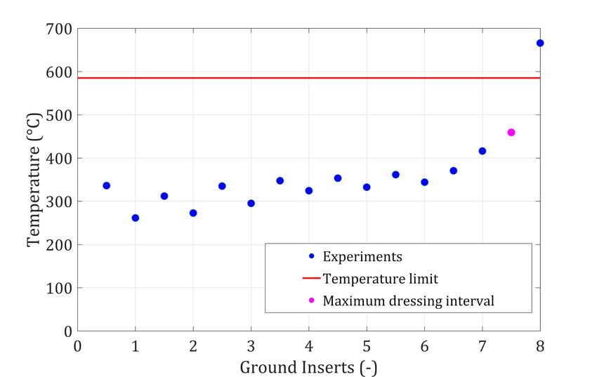
4

where µt,co (x) is the predicted mean cost function after t iterations obtained by Gaussian process regression using equation (4),
  2
σt,co (x) is the predicted variance of the cost after t iterations obtained by Gaussian process regression using equation (5), Cmin
                                                                                                           √ RZ
is the so far lowest measured cost, F (Z) is the cumulative standard normal distribution F (Z) = 1/ 2π −∞ exp −t2 /2)dt,
                                                                                             √
and φ(Z) is the probability density function of a standard normal distribution φ(Z) = 1/ 2π exp(−Z 2 /2). A standard normal
distribution is a normal distribution with zero mean and standard deviation of one. The acquisition function is displayed
exemplarily for a cost minimization problem in Figure 2(a) using the Gaussian process regression from Figure 1(a). Based
on the acquisition function the next experiment is conducted at a process parameter of 0.25, which maximizes the acquisition
function.
   Most machining operations require fulfilling constraints such as workpiece quality, process or safety constraints. As proposed
in [20], the expected improvement acquisition function can be extended to constrained optimization, which is used in this study,
                                                                       n
                                                                       Y
                                                  aEIC (x) = aEI (x)         pf,i (x)                                           (11)
                                                                       i=1

where aEI (x) is the expected improvement without constraints (9), n is the number of constraints, and pf,i is the probability
that the constraint i is fulfilled. Note that for the constrained case the best observed value Cmin is the minimal measured
cost value, which fulfills all constraints - and not the absolute minimal measured cost as in the case without constraints. The
probability that the constraint i is fulfilled can be calculated as follows,
                                                            Z λi
                                                                         −(t − µt,ci (x))2

                                                       1
                                       pf,i (x) =      √          exp          2 (x)         dt                             (12)
                                                  σt,ci 2π −∞                2σt,c i

where λi is the maximum allowed value for constraint i, µt,ci (x) is the predicted mean of constraint i after t iterations
                           2
calculated using (4), and σt,ci
                                (x) is the variance of the constraint i after t iterations calculated using (5). Here, the constraint
i is modeled again using Gaussian process regression and the predicted mean and uncertainty are used in the calculation. The
next experiment is conducted for process parameters x∗ , which maximize the constrained expected improvement acquisition
function.
                                                      x∗ = argmax aEIC (x)                                                       (13)
   Figure 2(b) shows exemplarily the result of a Gaussian process regression for a constraint quantity. In a real application,
the quantity might be surface roughness of the workpiece or the temperature during the grinding process and must stay below
a specified limit, which depends on the requirements such as the final workpiece quality. In this example,the limit is set to
250. The probability that the constraint is fulfilled is displayed in Figure 2(c) and can be calculated using equation (12) and
the Gaussian process regression of the constraint, as displayed in Figure 2(b). Finally, the constrained expected improvement
acquisition function is displayed in Figure 2(d) and can be calculated according to equation (11), using the Gaussian process
regression of the cost (displayed in Figure 1(a)) and the Gaussian process regression of the constraint (displayed in Figure 2(b)).
The constrained expected improvement acquisition function is maximal for a process parameter value of 0.61, which is the
next experimental parameter. The constrained expected improvement acquisition function favors higher process parameters than
the acquisition function without considering constraints because according to the Gaussian process regression of the constraint
the probability that low process parameters fulfill the maximum allowed constraint of 250 is low. After the next experiment is
conducted at a process parameter value of 0.61, the optimization procedure is repeated with the newly available measurements
until a maximum number of iterations or a stopping criterion is reached.

                                                       III. M ETHODOLOGY
A. Grinding operation
   The grinding operation is performed on an Agathon DOM Semi grinding machine (see Figure 3). An initial quadratic shaped
insert (14.5 mm x 14.5 mm x 4.76 mm) made of tungsten carbide (Tribo S25, grain size 2.5 µm, HV30 1470) is ground on
two opposite sides, resulting in a final insert geometry of 10 mm x 14.5 mm x 4.76 mm. The machine is equipped with a metal
bonded diamond grinding wheel with a mean diamond grain size of 46 µm and a grain concentration of C100 (D46C100M717
from Tyrolit). During grinding, the grinding wheel is oscillated with 1 Hz to ensure a uniform wear of the grinding wheel.
The spark-out time is set to 3 seconds and the oscillation during spark-out is slightly increased to 1.5 Hz. After the grinding
wheel is worn out, it is conditioned by a dressing wheel (89A 240 L6 AV217, geometry specification 150x80x32 W12 E15
from Tyrolit). For all experiments the dressing parameters were constant (dressing infeed is 0.1 mm, grinding wheel speed is
6 m/s, dressing wheel speed is 12 m/s, feed rate is 0.5 mm/min, and spark-out time is 1 sec). The used cooling lubricant is
Blasogrind HC 5 (from Blaser Swisslube) with a constant flow rate supplied by a multi-needle nozzle as shown in Figure 3.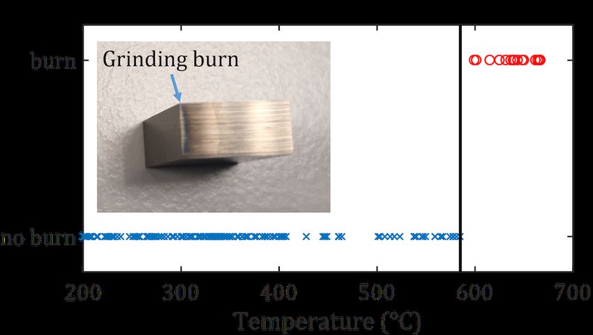
5

Fig. 2: Panel (a) shows the calculation of the acquisition function without considering constraints using equation (9) and the
Gaussian process regression model of the cost as displayed in Figure 1(a). Panel (b) shows the Gaussian process regression
model of the constraint exemplarily, calculated by maximizing the marginal log likelihood. Panel (c) shows the probability that
the constraint is fulfilled, calculated using equation (12) and the Gaussian process regression of the constraint, as displayed in
panel (b). Panel (d) shows the result of the acquisition function considering constraints, which can be calculated using equation
(11).

                                Fig. 3: Overview of grinding kinematic and experimental setup

B. Measurement set-up and process constraints
   High temperatures at the contact zone between grinding wheel and workpiece result in severe thermal damage of the
workpiece and in grinding burn. Grinding burn causes an undesired structure change of the workpiece material and must be
avoided. In addition, grinding with high temperatures may result in ignition of the grinding oil and results in potential hazardous
situations. In this study, grinding burn limited the maximum allowed temperature because grinding burn was observed at lower
temperatures than ignition of grinding oil. The temperature is measured optically using an optical fiber embedded inside the
grinding wheel, which collects the emitted radiation at the contact zone of the grinding wheel and the workpiece. Figure 4 shows
a schematic of the measurement equipment. The optical signal is evaluated on the rotating grinding wheel (pyrometer), filtered
and transmitted to a receiver unit outside the grinding machine and converted to temperature. In total, four optical fibers are
evenly distributed on the grinding wheel circumference for the temperature measurement. For each grinding operation, the final
considered temperature is averaged twice. First, the average of the ten highest temperature readings is calculated, followed by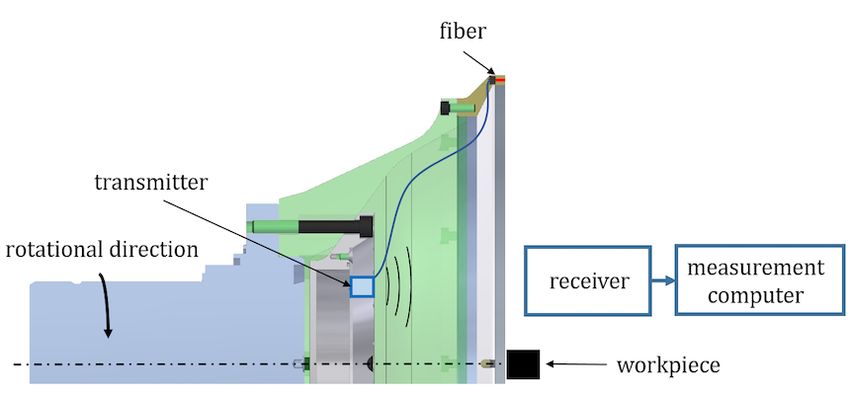
6

                                  Fig. 4: Schematic of embedded temperature measurement

                          Fig. 5: Grinding burn limit of preliminary experiments adapted from [21]

averaging the computed values for each sensor. Note that the evaluated temperature of the pyrometer depends on emissivity of
the measured surface. The temperature sensor was not calibrated, which allowed only for measurements of relative temperature.
As the temperature sensor is used to detect grinding burn with a burn threshold temperature determined in advance, having
access to relative temperatures proved sufficient for the goals of the grinding process optimization. If the first ground insert
side after dressing already is exposed to high temperature and grinding burn, the workpiece quality is not fulfilled for the
current and for the following workpieces, as in general the grinding temperature increases during grinding due to grinding
wheel dulling. The measured temperature of the first ground side after dressing is therefore a constraint in the subsequent
optimization procedure and should not exceed the allowed threshold value. The temperature readings after dressing were used
to determine the maximum dressing interval. The maximum dressing interval is defined as the number of grinding cycles until
the temperature exceeds the maximum allowed temperature. The experimental run was stopped when this temperature limit
was exceeded. To avoid unnecessary long experimental runs, the run was stopped after 8 inserts if the maximum temperature
was not previously exceeded. The maximum allowed temperature was set to 585◦ C because in preliminary experiments in
[21] with 194 insert sides grinding burn has been classified with a 100% success rate using this temperature measurement
system and the same workpiece-wheel combination as in this study. Figure 5 shows the classification of grinding burn based
on a temperature threshold and temperature measurements. In [21] grinding burn is detected optically by the black coloring of
the workpiece surface. This is a simple method for grinding burn detection which is often used in an industrial environment.
In this study, this approach is considered sufficient because it is only used to specify the maximum allowed temperature and
thereby the desired workpiece quality. For workpieces with higher quality requirements, the maximum temperature might be
determined based on more sophisticated methods, such as Barkhausen noise measurements as applied in [22].
   The surface roughness of the workpiece is measured transversal to the grinding direction and orthogonal to the cutting edge
using a tactile measurement device (Form Talysurf 120 L from Taylor Hobson) with a measurement tip radius of 2 µm. The
evaluation length was reduced to 4 mm because the total thickness of the insert was only 4.76 mm. The wavelength cut-off
is set to λc = 0.8 mm. In general, the roughness of both ground sides per insert is measured and averaged. If grinding burn
occurred on a ground side the roughness was not measured on this side. Instead, the roughness measurement was repeated at
a different location on the other ground side, where grinding burn did not occur. The roughness measurements change from
insert to insert with no clear trend. Therefore, in a conservative approach, the maximum measured roughness value of one
optimization run, grinding with a freshly dressed wheel until grinding burn occurred, was considered as a constraint for the
optimization. In this study, the roughness was limited to Ra,max = 230 nm.
7
TABLE I: Parameters for cost calculation
Parameter Description Value
Vg Removed material per workpiece 310.6 mm3
s Number of ground sides 2
apg Infeed per side 2.25 mm
td Dressing time 19 sec
agw Abrasive layer thickness of the grinding wheel 4 mm
ad,gw Wear of the grinding wheel during dressing 1 µm
adw Thickness of the dressing wheel 65 mm
ad,dw Wear of the dressing wheel during dressing 0.1 mm
Cm Machine hourly cost 100 U/h
Cgw Cost of grinding wheel 1500 U
Cdw Cost of dressing wheel 95 U
C. Cost calculation
The grinding operation cost cannot be measured directly with a single sensor as it is composed of both process-related
quantities such as grinding time and grinding wear, and of economic quantities such as machine hourly cost and cost of the
grinding wheel. The total cost to grind one insert is calculated based on grinding time cost, dressing time cost, cost of grinding
wheel wear during dressing, and cost of dressing wheel wear during dressing.
s · apg Cgw ad,gw Cdw ad,dw Vg
CT (vs , f ) = Cm + Cm td + + (14)
f agw adw Vw (vs , f )
The feed rate f , and the removed workpiece material until the wheel is dull Vw depend on the selected input parameters feed
rate f and cutting speed vs , which are the process parameters used in Bayesian optimization. The other cost parameters are
constants as summarized in Table I. The grinding wheel wear during dressing was considered and the wear during grinding was
neglected. This assumption is reasonable because it is known that metal bonded grinding wheels hold the diamond grains very
strongly, resulting in a high abrasive wear resistance whereby self-sharpening is limited [23]. The limited self-sharpening of
the grinding wheel requires redressing of the grinding wheel, which is assumed to be the main cause of grinding wheel wear.
The grinding wheel wear during dressing ad,gw was assumed to be 1 µm. Grinding wheel wear during dressing is determined
by the dressing parameters, which were fixed in this study and not considered in the optimization. In this study, grinding wheel
wear during dressing can be considered as a weight in the cost function. The spark-out time for each grinding operation was
not considered for cost calculation because it only shifts the cost function up by a constant value and does not influence the
optimal parameters. For generality, the cost is specified with units U.
D. Optimization Implementation
The objective in this study is to find the process parameters minimizing the total production cost CT and to fulfill the
maximum temperature constraint Tmax and the maximum surface roughness constraint Ra,max .
T (vs , f ) < Tmax
xmin = argmin CT (vs , f ) s.t. (15)
Ra (vs , f ) < Ra,max
In general, the optimization objective in machining is to minimize production costs, as applied in this study. However, other
objectives such as energy consumption or environmental impact may also be considered. The algorithm was implemented in
MATLAB using the GPML library [24] for Gaussian process regression. A flow diagram of the implementation is shown in
Figure 6. The optimization is started with two experiments at random process parameters within the input optimization domain.
The optimization domain for the Bayesian optimization was set based on experience to a minimal feed rate of 10 mm/min and
a maximum feed rate of 40 mm/min. The minimal cutting speed was set to 12 m/s and the maximum cutting speed was set
to 30 m/s. In this way, a typical cutting speed range was covered. After calculating the cost per part at the measured process
parameter values and determining the hyperparameters, three Gaussian process regressions are calculated, to model the cost,
the temperature, and the roughness.
Based on the obtained probabilistic predictions at different (not previously probed) values of the process parameters, the
optimal parameters that fulfill (15) can be calculated based on the obtained probability distributions for the cost, temperature
and roughness. Using stochastic models allows for probabilistic statements about the fulfillment of the constraint limits. As
discussed in detail in [25], the optimal parameters xopt = (vs,opt , fopt ) are calculated as the parameters, which minimize the
expected cost µt,co (vs , f ) after t experiments calculated using equation (4) and fulfill the roughness and temperature constraints
with probabilities higher than user defined values pRa,min and pT,min .
pf,T (vs , f ) ≥ pT,min
xopt = argmin µt,co (vs , f ) s.t. (16)
pf,Ra (vs , f ) ≥ pRa,min8
Fig. 6: Flow diagram of optimization implementation
The minimal probability that a constraint is fulfilled can be chosen freely and depends on the requirements. For example, many
parts for the aviation industry will require a high minimal probability that the constraints are fulfilled. On the other hand if
one produces disposable products it might be reasonable to accept a lower minimal probability that the constraints are fulfilled.
The probability pf,i that the constraint i is below its maximum allowed value λi can be calculated for temperature pf,T and
roughness pf,Ra by using equation (12) and the maximum allowed temperature value Tmax = 585◦ C and the maximum allowed
roughness value Ra,max =230 nm (specified in section III-B). In general, it is possible to specify separate minimal probabilities
for temperature and roughness. In this study, the parameters pT,min and pRa,min were set equal for simplicity.
Afterwards the optimal parameters can be used to assess convergence as proposed in [18],
2σt,co (xopt ) < (17)
where σt,co is the predicted standard deviation of the cost at predicted optimal parameters xopt after t iterations and is the
convergence limit. In this way, convergence is reached when 95% of the predicted cost values at optimal parameters are within
µc (xopt ) ± . The convergence limit must be higher than the combined cost measurement and process uncertainty, otherwise
convergence can never be reached. To increase the convergence robustness, full convergence is reached, when the stopping
criterion is below 0.04 U over three consecutive iterations, the optimal feed rate change within an interval of 0.4 mm/min, and
the optimal cutting speed change within an interval of 0.2 m/s. If convergence is not reached the next experimental parameters
will be determined based on maximizing the constrained expected improvement acquisition function and the optimization
continues.
IV. R ESULTS
Figure 7 shows a typical temperature reading as a function of ground inserts for a full experimental run with constant
input parameters. The grinding wheel was dressed before each experimental run, making it sharp and clean. In general, the
temperature is strongly influenced by the accumulated removed material volume, where towards the end of an experimental run
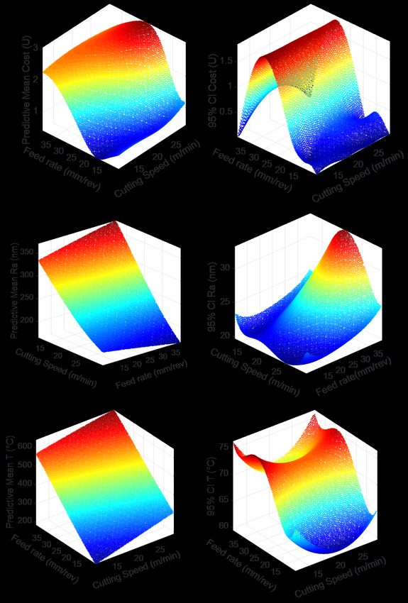
the temperature increases. The second side of the 8th insert does not fulfill the constraint, resulting in grinding burn. Therefore,9 Fig. 7: Typical temperature measurement as a function of ground inserts for a cutting speed of 24.3 m/s and a feed rate of 11.7 mm/min. The last side which fulfills the temperature constraint is the first side of plate 8. Therefore, the maximum dressing interval is 7.5 inserts. Fig. 8: Convergence of Bayesian optimization with a maximum allowed probability of quality defects pRa,min =pT,min =0.5 the measured maximum dressing interval for this parameter set is calculated as 7.5 inserts, which corresponds to an accumulated removed material volume Vw of 2329.5 mm3 . Depending on the grinding task, considering workpiece handling time may lead to positive natural numbers as optimal dressing intervals instead of positive real numbers due to timesaving of dressing and workpiece handling parallelization. In this study, handling time of workpiece was neglected because it is considered very short compared to the dressing time and strongly depends on the used handling system and corresponding parameters. Figure 8 and Figure 9 present the on-machine optimization. Convergence was judged for a minimal allowed probability of quality defects of 0.5 (pRa,min = pT,min = 0.5). The first two experiments are conducted at random points in the parameter space to initialize the optimization. The first and the second experiment do not fulfill the constraints, therefore the algorithm does not approach convergence after these experiments. However, the proposed trial for the third measurement is at high cutting speeds and low feed rates, which reduces both surface roughness and temperature. The third measurement fulfills the constraints. Until the 8th iteration the uncertainty of the prediction is reduced drastically. After the 8th iteration, the uncertainty remained low until full convergence is reached after 12 iterations. Experimentally, the best parameters are obtained at the 10th iteration with a cutting speed of 24.3 m/s, a feed rate of 11.7 mm/min, and a dressing interval of 7.5 inserts. After the 10th iteration, a small increase in the cost and the uncertainty is observed, however within the convergence limits. The blue line on Figure 8 shows the current measured cost values. Experimental points explored due to high model uncertainty often result in high costs, for example iterations 4, 7, and 9. In such cases, often the constraints are not fulfilled. Figure 10 shows the predicted mean and confidence interval after 12 iterations for cost, roughness and temperature. The predicted cost is high for low feed rates because the operation is time consuming. On the other hand, higher feed rates lead to shorter dressing intervals, which makes redressing expensive. Optimal parameters are a trade-off between these two costs. After 12 experiments, the model uncertainty in the high feed rate range (above 25 m/min) is higher than the uncertainty corresponding to low feed rate. Considering the high predicted costs for these parameters, the uncertainty is still moderate. The roughness mostly depends on the cutting speed. An increase in cutting speed reduces the surface roughness whereas the feed rate only influences the roughness minimal. This is in line with the findings of the preliminary study [21] for cup wheel grinding with the same setup, where an extensive series of experiments was conducted. The predicted uncertainty of the roughness is between 19.7 and 33.4 nm, which is 9 and 15% of the maximum allowed roughness. An increase in feed rate or cutting speed leads to higher temperatures, again confirming the results reported in [21]. The predicted temperature uncertainty is between 59.5
10

Fig. 9: Conducted experiments after 12 iterations. Experiment with lowest cost and fulfilled constraints was 10th experiment

TABLE II: Optimal predicted parameters after 12 iterations with different minimal probabilities that the temperature and
roughness constraints are fulfilled. The predicted optimal costs and the predicted 95% confidence interval of the optimal costs
is also given.
                                       Minimal probability that
                                       constraints are fulfilled (%)     Optimal parameters                            Costs (U)
                                       50                                f   =   12.0   mm/min,   v   =   23.8   m/s   0.78±0.04
                                       84.1                              f   =   11.8   mm/min,   v   =   25.2   m/s   0.83±0.05
                                       97.7                              f   =   11.4   mm/min,   v   =   26.8   m/s   0.92±0.07
                                       99.9                              f   =   11.6   mm/min,   v   =   28.8   m/s   1.08±0.13

and 76.5◦C which is between 10 and 13% of the maximum allowed temperature. The temperature uncertainty is higher for
high feed rates because only limited number of experiments were conducted at high feed rates due to high total costs at high
feed rates. In such cases, the recommended process parameter configuration by the BO algorithm for the next trials moves to
process parameters corresponding to lower costs, and the more unfavorable regions of the parameter space are not extensively
explored.
   Table II shows optimal parameters for several different values of pRa,min and pT,min , computed from equation 16 after
12 iterations. The algorithm recommends an increase in cutting speed when the minimal probabilities that the constraints are
fulfilled pRa,min and pT,min are increased, without a large modification of the feed. An increase in cutting speed leads to
lower surface roughness and less probability to violate the surface roughness constraint. As expected, increasing the minimal
probability that the constraints are fulfilled results in higher production costs.

                                                                       V. C ONCLUSION
  In this study, Bayesian optimization with on-machine measurements was used to obtain optimal parameters for grinding
within a few iterations, while fulfilling quality and safety constraints. Gaussian process regression models were successfully
applied to model costs, roughness, and temperature of the grinding process. The proposed approach is suitable to consider the
probability that the constraints are fulfilled in the calculation of optimal parameters. In future, additional input parameters such
as dressing feed rate, dressing wheel speed, and grinding wheel oscillation frequency might be included in the optimization.
Furthermore, the optimization will benefit from additional sensor feedback such as grinding wheel wear sensors and integrated
cutting edge roughness measurements.

                                                               C ONFLICT OF INTEREST
  Agathon AG filed a patent on parts of this work.

                                                                        R EFERENCES
 [1] W. B. Rowe, L. Yan, I. Inasaki, and S. Malkin, “Applications of artificial intelligence in grinding,” CIRP Annals, vol. 43, no. 2, pp. 521 – 531, 1994.
 [2] C. W. Lee, “A control-oriented model for the cylindrical grinding process,” The International Journal of Advanced Manufacturing Technology, vol. 44,
     no. 7-8, pp. 657–666, 2009.
11
Fig. 10: Predicted mean cost (top left), cost confidence interval (top right), predicted mean roughness (middle left), roughness
confidence interval (middle right), predicted mean temperature (bottom left), and temperature confidence interval (bottom right)
after 12 iterations.
[3] H. E. Jenkins and T. R. Kurfess, “Adaptive pole-zero cancellation in grinding force control,” IEEE Transactions on control systems technology, vol. 7,
no. 3, pp. 363–370, 1999.
[4] R. V. Rao, “Modeling and optimization of machining processes,” in Advanced Modeling and Optimization of Manufacturing Processes. Springer, 2011,
pp. 55–175.
[5] C. W. Lee, “Dynamic optimization of the grinding process in batch production,” in ASME 2008 International Manufacturing Science and Engineering
Conference collocated with the 3rd JSME/ASME International Conference on Materials and Processing. American Society of Mechanical Engineers
Digital Collection, 2008, pp. 485–494.
[6] M. H. Gholami and M. R. Azizi, “Constrained grinding optimization for time, cost, and surface roughness using nsga-ii,” The International Journal of
Advanced Manufacturing Technology, vol. 73, no. 5-8, pp. 981–988, 2014.
[7] H. Tönshoff, T. Friemuth, and J. C. Becker, “Process monitoring in grinding,” CIRP Annals, vol. 51, no. 2, pp. 551–571, 2002.
[8] M. N. Morgan, R. Cai, A. Guidotti, D. R. Allanson, J. Moruzzi, and W. Rowe, “Design and implementation of an intelligent grinding assistant system,”
International Journal of Abrasive Technology, vol. 1, no. 1, pp. 106–135, 2007.
[9] T. Choi and Y. Shin, “Generalized intelligent grinding advisory system,” International journal of production research, vol. 45, no. 8, pp. 1899–1932,
2007.
[10] D. Barrenetxea, J. I. Marquinez, J. Álvarez, R. Fernández, I. Gallego, J. Madariaga, and I. Garitaonaindia, “Model-based assistant tool for the setting-up
and optimization of centerless grinding process,” Machining science and technology, vol. 16, no. 4, pp. 501–523, 2012.
[11] S. Shaji and V. Radhakrishnan, “Analysis of process parameters in surface grinding with graphite as lubricant based on the taguchi method,” Journal of
Materials Processing Technology, vol. 141, no. 1, pp. 51–59, 2003.
[12] C. K. Williams and C. E. Rasmussen, Gaussian processes for machine learning. MIT press Cambridge, MA, 2006, vol. 2, no. 3.
[13] B. Shahriari, K. Swersky, Z. Wang, R. P. Adams, and N. De Freitas, “Taking the human out of the loop: A review of bayesian optimization,” Proceedings
of the IEEE, vol. 104, no. 1, pp. 148–175, 2015.12
[14] J. Snoek, H. Larochelle, and R. P. Adams, “Practical bayesian optimization of machine learning algorithms,” in Advances in neural information processing
systems, 2012, pp. 2951–2959.
[15] H. Abdelrahman, F. Berkenkamp, J. Poland, and A. Krause, “Bayesian optimization for maximum power point tracking in photovoltaic power plants,”
in 2016 European Control Conference (ECC). IEEE, 2016, pp. 2078–2083.
[16] D. J. Lizotte, T. Wang, M. H. Bowling, and D. Schuurmans, “Automatic gait optimization with gaussian process regression.” in IJCAI, vol. 7, 2007, pp.
944–949.
[17] M. Maier, A. Rupenyan, M. Akbari, R. Zwicker, and K. Wegener, “Turning: Autonomous process set-up through bayesian optimization and gaussian
process models,” Procedia CIRP, vol. 88, pp. 306–311, 2020.
[18] M. Maier, R. Zwicker, M. Akbari, A. Rupenyan, and K. Wegener, “Bayesian optimization for autonomous process set-up in turning,” CIRP Journal of
Manufacturing Science and Technology, vol. 26, pp. 81–87, 2019.
[19] J. Mockus, V. Tiesis, and A. Zilinskas, “The application of bayesian methods for seeking the extremum,” Towards global optimization, vol. 2, no.
117-129, p. 2, 1978.
[20] J. R. Gardner, M. J. Kusner, Z. E. Xu, K. Q. Weinberger, and J. P. Cunningham, “Bayesian optimization with inequality constraints.” in ICML, 2014,
pp. 937–945.
[21] M. Maier, T. Gittler, L. Weiss, C. Bobst, S. Scholze, and K. Wegener, “Sensors as an enabler for self-optimizing grinding machines,” MM Science
Journal, vol. 2019, no. 04, pp. 3192–3199, 2019.
[22] B. Karpuschewski, O. Bleicher, and M. Beutner, “Surface integrity inspection on gears using barkhausen noise analysis,” Procedia Engineering, vol. 19,
pp. 162–171, 2011.
[23] I. D. Marinescu, W. B. Rowe, B. Dimitrov, and H. Ohmori, “9 - abrasives and abrasive tools,” in Tribology of Abrasive Machining Processes (Second
Edition), second edition ed., I. D. Marinescu, W. B. Rowe, B. Dimitrov, and H. Ohmori, Eds. Oxford: William Andrew Publishing, 2013, pp. 243 –
311.
[24] C. E. Rasmussen and H. Nickisch, “Gaussian processes for machine learning (gpml) toolbox,” Journal of machine learning research, vol. 11, no. Nov,
pp. 3011–3015, 2010.
[25] D. Dentcheva, “Optimization models with probabilistic constraints,” in Lectures on Stochastic Programming: Modeling and Theory. SIAM, 2009, pp.
87–153.You can also read