ORDER PARAMETER BASED STUDY OF HIDDEN UNIT SPECIALIZATION IN NEURAL NETWORKS FOR RELU AND SIGMOIDAL ACTIVATION FUNCTIONS
←
→
Page content transcription
If your browser does not render page correctly, please read the page content below
Faculty of Science and Engineering

           Neha Rajendra Bari Tamboli

    Research Internship in Computing Science

                       Supervisors

                 Prof. Dr. Michael Biehl

                  M.Sc Michiel Straat

  Order parameter based study of
Hidden unit specialization in Neural
 Networks for ReLU and Sigmoidal
       activation functions

                      October 2020

Bernoulli Institute for Mathematics, Computer Science and
                  Artificial Intelligence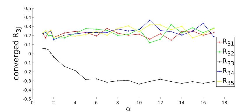
Chapter 1

Introduction

The recent popularity in deep learning has opened an advanced gateway to solving the state-

of-the-art subset of dynamic tasks like object detection and speech recognition. This subset of

tasks occur across various domains like stock market, medical science and military applications.

Deep learning allows computational models that are composed of multiple hidden layers to learn

representations of data with multiple levels of abstraction (LeCun et al. 2015). Shallow neural

networks consist of one hidden layer instead of multiple hidden layers. These form a toy-model

which can be exactly solved to study deep neural networks which have largely been used as

black boxes (Angelov and Sperduti 2016, Goodfellow et al. 2016, Prajit Ramachandran 2017).

In this work we study the generalization properties of a shallow neural network as a function

of the size of the dataset. We consider a student-teacher model training scenario in which we

train the student network and observe the overlap between its weights and the weights of the

teacher neural network. In order to understand the learning behaviour of the student neural

network, we invoke the celebrated statistical mechanics (Gibbs 1902) theory of physics which

gives us the tools to understand the macroscopic behaviors of a system using certain averages

over the properties of the microscopic constituents of the system. Specifically, we use statistical

mechanics inspired method of tracking the order parameters to spot a phase transition in the

network. These order parameters enable us to track the learning behaviour without having to

track the individual weights, i.e. they give us a macroscopic view of learning. The activation

functions used for this experiment are the ReLU and the shifted sigmoid. We analyse systems

of two different sizes and observe differences in student’s learning behaviour for these activation

functions. We also make comparison with theoretical results based on statistical mechanics of

                                                1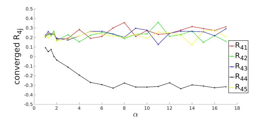
Chapter 1. Introduction

equilibrium and the central limit theorem.

                                             2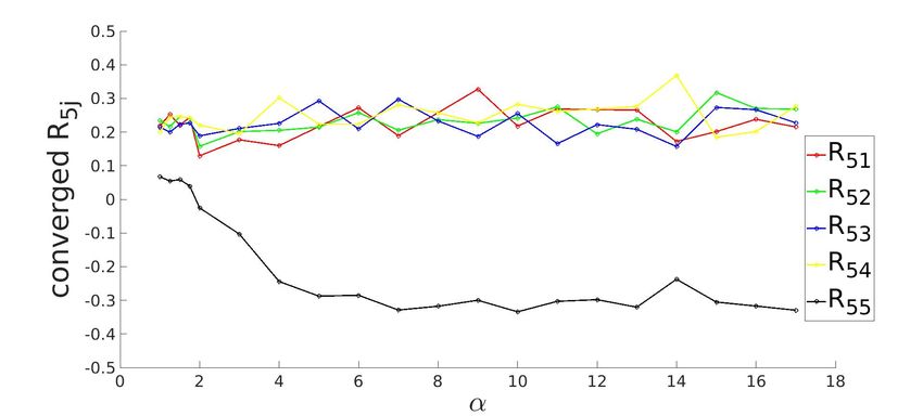
Chapter 2

Methods

2.1    Experiment Setup

We consider a shallow artificial feed-forward neural network with one hidden layer comprising

of K hidden units, N input units and one linear output unit. The input nodes are connected

to each hidden unit via edges that have adaptive weights. Therefore there are N × K weights

between input and hidden units and K weights between hidden to output unit. Weights can be

aggregated as weight vectors by introducing the notation wk ∈ RN , whose components include

all weights going to the k th hidden unit, where k = 1..K. The hidden unit performs a weighted

sum of the components and normalization of input vector followed by the application of an

activation function. Weights connecting hidden to output units are all unity. Therefore, the

output simply adds the incoming activations and normalizes the sum.

The main aim is to study how closely the weights of a neural network called ”student” resem-

ble another neural network called ”teacher”, upon training. The teacher neural network has

randomly generated weights, identical architecture and is not trained. Moreover, the student

neural network is trained on the labels generated by the teacher. The aim of the learning is not

only to learn the examples, but to learn the underlying function that produces the targets for

the learning process (Krogh and Hertz 1992).

                                               3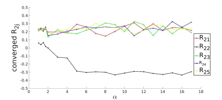
2.2. Activation function Chapter 2. Methods
Figure 2.1: Schematic representation of the architecture of student and teacher neural networks
with N input units, one hidden layer with K = 2 units and one linear output unit. The
individual neurons in the hidden unit execute a weighted sum of inputs to compute
√ the local
potential xk and apply an activation function g on it. The sum is normalized by N to keep the
norm of the local potential of O(1). The output √neuron acts as an aggregator and computes the
sum of activations. This sum is normalized by K such that it approaches O(1). The output
is given by σ(ξ) and is continuous. This neural network thus performs regression.
2.2 Activation function
The main goal of this report is to study generalization properties of the student neural network
under two different types of activation functions. The first one called Rectified Linear Unit
(ReLU) is defined as max(0, x):
0,
if x < 0,
g(x) = (2.1)
x
elsewhere.
Therefore the function maps R → R+ , making it unbounded. The derivative of ReLU is defined
as follows:
0, if x < 0,
g 0 (x) = (2.2)
1
if x > 0.
The ReLU activation function is not differentiable at x = 0, however this does not affect us
computationally because of floating point precision. In our simulations we define the derivative
to be 1 at x = 0. This function is also called the ramp function and is analogous to half
4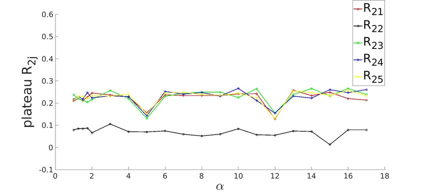
Chapter 2. Methods                                                          2.2. Activation function

wave rectification in electrical engineering. This activation function has strong motivation from

biology (Hahnloser et al. 2000).

        (a) The ReLU activation function.             (b) Derivative of the ReLU activation function.

Figure 2.2: The ReLU activation function and its derivative. The x-axis represents the local
potential.

The advantages of ReLU activation function includes:

   • biological plausibility.

   • efficient computation & sparse representation.

   • fewer vanishing gradient problems compared to sigmoid which saturates asymptotically

      in both directions (fig2.3).

   • scale invariance: max(0, γx) = γmax(0, x) for γ > 0.

The second activation function is the sigmoid activation function. For the purpose of this work

we use the shifted erf (Ahr et al. 1998) function defined as:

                                                    x
                                     g(x) = 1 + erf √ .                                          (2.3)
                                                      2

Its derivative is given by:                       r
                                            0         2 −x2
                                        g (x) =         e 2 .                                    (2.4)
                                                      π

The shifted sigmoid activation function maps R → [0, 2], making it bounded. Additionally, the

function is differentiable everywhere and monotonically increasing.

                                                  5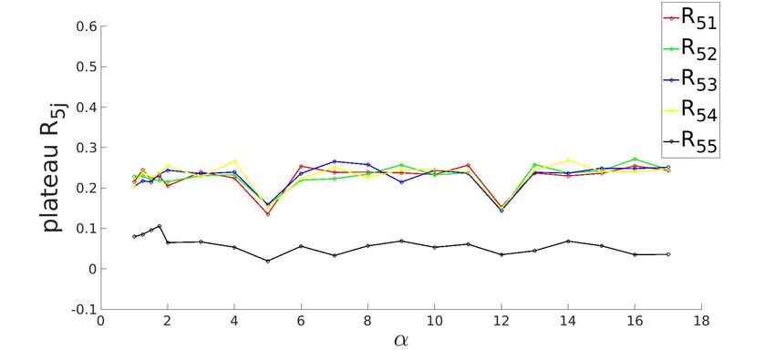
2.3. Student-teacher scenario Chapter 2. Methods
(b) The gaussian derivative of erf activation func-
(a) The erf activation function.
tion.
Figure 2.3: The shifted sigmoid activation function realised as a shifted erf function and its
derivative.
2.3 Student-teacher scenario
This experiment involves two networks namely, the Student and the Teacher network. They
have similar architecture shown in fig 2.1. We randomly generate the weights of the teacher
neural network. These weights are drawn from a normal distribution and are denoted by
wk∗ ∈ RN . The teacher network acts on the input data to generate a label, which is what the
student network is eventually trained on. The randomly generated teacher weight vectors are
orthonormalized using the Gram-Schmidt procedure (Golub and Van Loan 1996).
1, if m = n,
∗ ∗
wm · wn = δmn , where δmn = (2.5)
0, if m 6= n
is the kronecker delta function. Input vector corresponding to the µth example is given by ξ µ .
Each input vector is N dimensional to make it commensurate with the dimension of the input
layer of the neural network. Furthermore, we choose ξ µ such that each component is drawn
from a normal distribution, just like the weights.
The training set matrix used to train the student network is D = {ξ µ , τ µ }P1 , where τ represents
the teacher network generated label. Here, P is the number of examples.
The quantity
6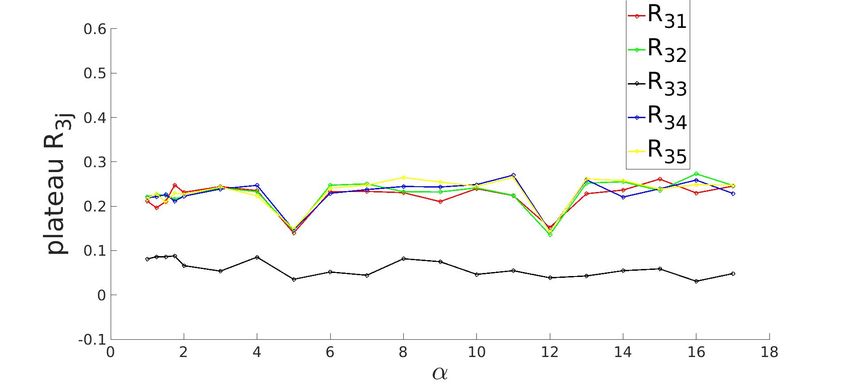
Chapter 2. Methods                                                2.3. Student-teacher scenario

                                                 P
                                           α=                                              (2.6)
                                                KN

scales the number of examples in the dataset as P = α K N . The detailed effects of increase

in the number of examples on learning is elaborated in the results section.

The local potential for the teacher network is represented by

                                              1
                                       x∗m = √ wm
                                                ∗
                                                  ·ξ                                       (2.7)
                                              N

       ∗ is the weight vector corresponding to the mth hidden unit and m = 1..M , where M
where wm

are the number of hidden units in the teacher network . The local potential is fed to the choice

of activation function and then aggregated by the output unit to generate the output label

                                                M
                                             1 X
                                    τ (ξ) = √     g(x∗m )                                  (2.8)
                                              M m

where, τ is the final teacher output. For the sake of simplicity, the current simulation deals

with K = M . Other configurations where K 6= M can also be studied but are not covered here.

                                                7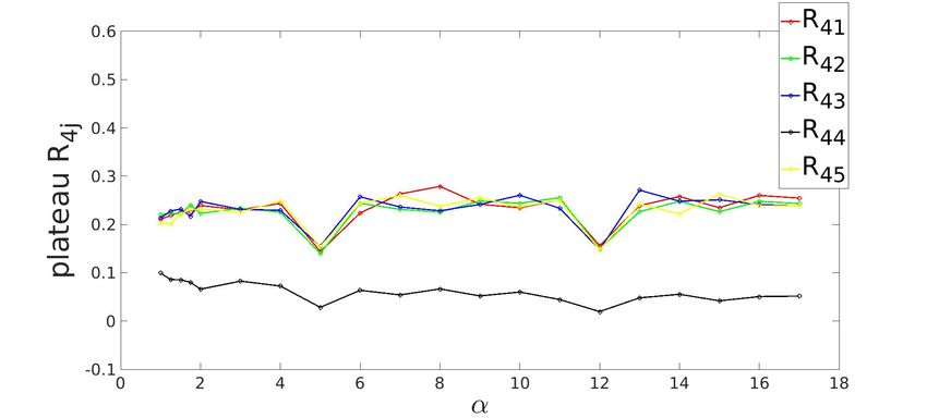
2.4. Loss function                                                            Chapter 2. Methods

2.4     Loss function

The cost that penalizes the errors is represented in terms of the quadratic loss function (Berger

1985). The cost determines how good the student is at predicting teacher labels. The cost

function is represented as,

                                           1
                                     (ξ) = (σ(ξ) − τ (ξ))2                                 (2.9)
                                           2

Cost function is applied on each example where σ(ξ) is the student output and τ (ξ) is the

teacher output per example. The cost calculated is then summed over for all the examples to

calculate the training error for the entire training set. It is defined as below,

                                               P
                                               X
                                          E=         (ξ µ ).                              (2.10)
                                               µ=1

where ξ refers to the current example input vector taken into consideration for computing the

cost.

                                                 8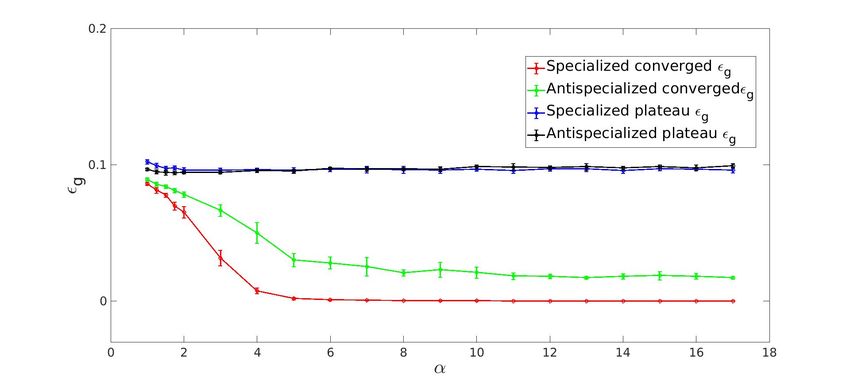
Chapter 2. Methods                                                   2.5. Stochastic Gradient Descent

2.5      Stochastic Gradient Descent

The student neural network is trained using the stochastic gradient descent (SGD) algorithm

(Robbins and Monro 1951), to estimate the parameters of the student adaptive weights iter-

atively, that minimize the cost function. During each iteration in the training process, the

network starts from a randomly selected example ξ from a set of P examples, it then computes

the student label σ(ξ) using forward propagation to calculate the cost function. The teacher

label is pre-calculated for every example. It then moves the weights by a step proportional to

the negative of the gradient of the cost function with respect to the weights (i.e. in the direction

of steepest descent of the cost function). At the training step i + 1 when a particular example

ξ is chosen, the weight matrix is given by,

                                                     η∇wi (ξ)
                                    wi+1
                                     k   = wik −             k
                                                                 .                             (2.11)
                                                         N

for k = 1...K. Here, η is called the learning rate. After, every step the student weight vector

associated with the hidden unit j is normalized as below:

                                                     √
                                              wk =       N                                     (2.12)

SGD performs frequent updates with a high variance that cause the objective function to fluc-

tuate heavily (Ruder 2016). Therefore tuning a reasonable learning rate η is important. If η

is too large, the network will fluctuate far from the global minima and never converge. If η is

too small the network will never learn. In our experiments we heuristically tuned η to be equal

to 0.5 and 0.8 for different systems. The learning process is terminated when the decrease in

the loss function for a set prolonged period of time is negligible or when a required number of

training steps have been taken. To evaluate the derivative of the loss function (2.10) w.r.t to

the weights we invoke the celebrated backpropagation method (Rumelhart et al. 1986, Kelly

1960):

                                   ∇wi  = (σ − τ )g 0 (wik · ξ)ξ                              (2.13)
                                       k

                                                 9
2.6. Generalization error Chapter 2. Methods
The training process is described in the pseudocode below;
Listing 2.1: Psuedocode for NN training using Stochastic gradient descent
for i to training steps :
% one random example at a time
example = randi ( dataset ) ;
% forward prop
local_potential = dot ( example , weights ) /(\ sqrt ( N ) )
psi ( example ) = sum ( activation_function ( local_potential ) ) /(\ sqrt ( K ) )
% backprop
gradient = ( psi ( example ) - tau ( example ) ) * derivative ( local_potential ) *
example ;
% update
new_weights ( example ) = ( weights ( example ) ) - (( learning_rate / N ) *
gradient ) ;
% weight normalization
new_weights ( example ) = new_weights ( example ) ./ norm ( new_weights ( example ) )
;
end
2.6 Generalization error
The generalization error measures the degree to which a neural network is able to adapt itself
on a novel dataset. The network should not only learn the training data, but it should be able
to predict labels on novel data (test data). If a network performs well on the training data but
does not generalize well on the unseen data, the model is said to overfit. When the network
does not train well on the training dataset and neither does it generalize well on the unseen
data, it is commonly referred to as under-fitting. The goal is to reduce the generalization error
without under-fitting or over-fitting the model.
The mathematical model for generalization error is represented as
* K K
+
1 X X 2
g = g(xi ) − g(x∗j ) (2.14)
2K
ı=1 =1
The generalization error is the expectation value of the quadratic deviation between the student
and the teacher output. It computes the average over the joint density over xi & x∗j which
fundamentally is a gaussian average. The gaussian average can be computed in terms of the
order parameters for both ReLU (A.1) (Michiel Straat 2018, Oostwal et al. 2021) and sigmoid
10Chapter 2. Methods 2.7. Order parameters
(A.2) (Saad and Solla 1995).
2.7 Order parameters
An order parameter distinguishes two different phases (or orders). Typically an order parameter
has different values for different phases. For our experiments, we need to keep track of how
student weights change as learning progresses. Here, order parameters come in handy as a few
of them are sufficient to describe learning in large systems. We now derive order parameters
(Biehl et al. 1998, Ahr et al. 1998) from weight vectors to track the progress in learning.
The order parameter Qij is the student overlap, defined as:
wi · wj
Qij = (2.15)
N
and
1,
if i = j,
Qij = (2.16)
C,
if i 6= j.
The overlap between identical student vectors is 1, while non-identical students overlap at a
scalar value C.
Similarly, the order parameter Rij is the student-teacher overlap.
wi · wj∗
Rij = (2.17)
N
and,
R, if i = j,
Rij = (2.18)
S,
if i 6= j.
The assumptions in equations (2.16) and (2.18) simplify the consideration of specialization as
well as anti-specialization of the hidden units. The special consideration of i = j singles out
one optional specialization but all the others are equivalent.
The phases can be represented as below;
112.8. Training of Student Neural Network Chapter 2. Methods
The R = S phase represents a barren plateau, in this phase the neural network does not
specialize in learning. All the student vectors have equal overlap with all the teacher vectors,
due to which they never really learn in respect to a single teacher.
The R > S represents specialization, i.e. as per equation (2.18), the i = j student-teacher
pair have maximum overlap with each other and the student learns with respect to their equal
indexed teacher vector.
The R < S represents anti-specialization. As per equation (2.18), the student vector shows
minimum overlap (negative) with the teacher vectors when the index i = j, where as the
student vector is weakly positively overlapped with the teacher vectors such that index i 6= j.
The normalization and orthogonal property of the student and teacher weight vectors as per
(2.12) and (2.5) obey the property that the generalization error can be represented in terms of
order parameters as (A.1) and (A.2). The order parameters lie between -1 and 1.
− 1 ≤ Qij , Rij ≤ 1 (2.19)
2.8 Training of Student Neural Network
The plots in fig 2.4 depict the training of a student neural network in the student teacher
scenario using stochastic gradient descent. We use the ReLU activation function in the hidden
units. The first plot depicts the generalization error g as a function of training steps. We can
clearly spot a plateau region where the graph g is almost flat. Additionally, both diagonal
and off-diagonal elements of Rij have essentially the same values signalling poor generalization.
As training steps progress, the system eventually specializes well, as evident from the diagonal
values of Rij i.e. R11 and R22 reaching their maximum value of 1 and off-diagonal elements
R12 and R21 reaching 0. This results in a further decrease of g and eventual convergence to
≈ 10−6 . The training error E follows a trend similar to g . In the fig 2.5, we report similar
plots for α = 1. Here, we see that both g and E stagnate into a plateau state, i.e. the student
network never generalizes well. This is evident from looking at the student-teacher overlap Rij
vs training steps. The diagonal elements of Rij saturate at 0.5, instead of going to 1 and the
off diagonal elements saturate at around 0.2, instead of going to zero. To obtain these plots
the values N, η and the number of training steps were chosen heuristically after several trials.
12Chapter 2. Methods 2.8. Training of Student Neural Network
The generalization achieved in this training is very sensitive to α which controls the dataset
size P . Studying the behaviour of student neural network as a function of α is the central goal
of this report. Armed with statistical mechanics inspired tools, i.e. the student-teacher order
parameter Rij , we report the learning curves in the next section.
Figure 2.4: Training of student neural network with N = 100 input units, K = 2 hidden units
at a dataset size scaling parameter α = 8 and learning rate η = 0.5 using stochastic gradient
descent. Top plot depicts the generalization error g as a function of training steps. Middle
plot depicts student-teacher overlap parameters Rij . Bottom plot depicts training error E as a
function of training steps. At the end of the training the g = 5.135×10⁻⁶ and E = 2.8964×10⁻⁶ .
132.8. Training of Student Neural Network Chapter 2. Methods
Figure 2.5: Training of student neural network with N = 100 input units, K = 2 hidden units
at a dataset size scaling parameter α = 1 and learning rate η = 0.5 using stochastic gradient
descent. Top plot depicts the generalization error g as a function of training steps. Middle
plot depicts student-teacher overlap parameters Rij . Bottom plot depicts training error E as
a function of training steps. At the end of the training the g = 0.1069 and E = 0.0052. The
g decreases rapidly initially, but eventually stagnates and the plateau state appears to be the
only solution.
14Chapter 3
Results
In this section we will report the generalization error achieved by the student network as a
function of α for two different hidden layer sizes K = 2 and K = 5. Additionally, to understand
the behaviour of student units w.r.t. the teacher units we will report the student-teacher overlap
order parameters as a function of α. The K = 2 system serves as the first example where a
phase transition between states with poor generalization and states with good generalization is
spotted qualitatively. In the research leading to this report we studied systems with K = 2 to 5.
However, it’s the K = 5 system where we first see anti-specialization behaviour for ReLU
activation function. Phase transitions are spotted in this system simulation as well, at least
qualitatively.
We begin by reporting the initial conditions which lead to specialization and anti-specialization
behaviour for different systems.
3.1 Initial conditions
Initial conditions play a crucial role in determining if the system will specialize or anti-specialize.
3.1.1 Specialization
For achieving a specialized state where R and Q follow the conditions as per (2.18 and 2.16)
the initial condition for K = 2 and K = 5 systems for both ReLU and sigmoid are,
Q = (IK×K ) and R = 0.2(IK×K ). (3.1)
153.2. Simulation of learning in matched student-teacher scenario Chapter 3. Results
where Qii = 1 and Qij = 0 for i 6= j while Rii = 0.2 and Rij = 0 for i 6= j.
3.1.2 Anti-specialization
In Anti-specialization the student vectors are anti aligned with corresponding teacher vector
(i.e. their dot product is negative). The student learns the adaptive weights of corresponding
teacher with which it has highest negative dot product. The initial conditions used for anti-
specialization are as below for K = 5 system.
Q = IK×K + (0.04)(JK×K − IK×K ); (3.2)
R = −0.001IK×K + (0.1)(JK×K − IK×K ); (3.3)
Where J is a matrix of all ones. Here, the student vector has a unity overlap with itself (Qii = 1)
and it has a non-zero overlap with the other student vectors (Qij = 0.4 for i 6= j).
R parameter configuration satisfies the condition R < S for anti-specialization. Equation (3.3)
shows that the corresponding (i = j) student-teacher vectors are negatively aligned while the
remaining vectors are weakly positively aligned. The student vector has an overlap of -0.0010
with its corresponding teacher vector (Rii ) and it has a non-zero overlap of 0.1000 with the
remaining teacher vectors (Rij for i 6= j).
The conditions laid out were found through trial and error using intuition from the definition
of order parameters.
3.2 Simulation of learning in matched student-teacher scenario
We now report the main results on learning in the student neural networks in the matched
student-teacher scenario. In these simulations we use N = 100 and 600, K = 2 and 5 and a
learning rate of 0.5 and 0.8. For reference, a system with K = 5, N = 600 and α = 20, implies
a dataset size of P = αKN = 60, 000 examples . For the system size K = 2 we repeat the
simulation for 30 iterations for 25,000 training steps for each alpha and report the averages
along with standard deviation (error bars). For larger system size i.e. K = 5 we repeated the
16Chapter 3. Results 3.2. Simulation of learning in matched student-teacher scenario
simulations for 10 iterations for 90, 000 training steps for each alpha. The number of iterations
here is less because of the time required to conduct these simulations.
3.2.1 Generalization Error for K=2 system
For the case K = 2 we obtain the learning curves for perfectly matching student-teacher scenario,
shown in fig 3.1. To produce these plots we followed the recipe laid out in the previous section,
for every α. Plot (a(b)) of fig 3.1 shows g as a function of α for the ReLU(sigmoid) activation
function. Here, we take the g value at the mid-point (midpoint of the region where the loss
values are almost constant) of the plateau as shown in fig 2.4. For the converged g we simply
take the end-point.
3.2.2 Converged and plateau states for K=2 system
Using the initial conditions for the K = 2 system (3.1.1), during the learning process the neural
network gets stuck in the plateau states initially. This is an unspecialized state and can be
observed in the figure (3.2a) for ReLU from α ≈ 1 to α ≈ 3 and in figure (3.2c) for sigmoid
from α ≈ 5 to α ≈ 6 approximately where R and S barely vary. Both the student hidden units
learn little information about the corresponding teachers.
Once the plateau states are overcome, the student network starts learning more efficiently.
Theory from (Oostwal et al. 2021) predicts that a phase transition occurs in this regime. Each
student vector largely overlaps with exactly one teacher vector. This represents the specialized
phase where Rij = 1 for i = j and zero for i 6= j. This can be observed for ReLU in (3.2a) for
α ≈ 4 and for sigmoid in (3.2c) for α ≈ 6.
The generalization error (3.1) starts to rapidly decrease when the student units start to special-
ize. Predictions from theory (Oostwal et al. 2021) are more precise as there the authors use the
limit N → ∞, there a sharp kink appears due to the large system size. After the kink, the g
decreases rapidly. In the plot above, the g converges to 7.845e − 11 for α = 16 for ReLU and
to 1.4611e − 04 for sigmoid at α = 23.
173.2. Simulation of learning in matched student-teacher scenario Chapter 3. Results
(a) g for ReLU
(b) g for Sigmoid
Figure 3.1: The generalization errors of converged and plateau states g for ReLU and sigmoid
activation function with K = 2 hidden units as a function of α. The plateau(converged) states
are unspecialized and lead to worse(better) generalization.
18Chapter 3. Results 3.2. Simulation of learning in matched student-teacher scenario
(a) ReLU converged (b) ReLU plateau
(c) Sigmoid converged (d) Sigmoid plateau
Figure 3.2: The student-teacher overlap order parameters Rij for student teacher system where
both system have 2 hidden units as a function of α (which governs the dataset size). The
converged parameters(a,c) show that after an initial period of bad generalization, the diagonal
order parameters approach 1 and the off-diagonal parameters approach 0, signalling specializa-
tion. For the plateau states, order parameters saturate at 0.5, signalling that no specialized
solution is achieved.
193.3. K=5 system Chapter 3. Results
3.3 K=5 system
We now move to a larger system size. Here we report the plots of student-teacher overlap matrix
Rij with ReLU activation first and then the generalization error. Then we report results for
the sigmoid activation function in a similar fashion. For a K = 5 system the R matrix has 25
entries. To make comparisons easier we plot all doagonal elements with black color.
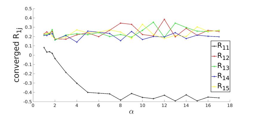
3.3.1 Converged state for K=5 system with ReLU activation function
(a) R1j (b) R2j
(c) R3j (d) R4j
(e) R5j
Figure 3.3: Row-wise plot of student-teacher overlap order parameter matrix at the converged
g . The diagonal elements of Rij (in black) approach the value of 1 and off-diagonal elements
approach 0 as α increases, signalling specialization.
20Chapter 3. Results 3.3. K=5 system
3.3.2 Plateau state for K=5 system with ReLU activation function
(a) R1j (b) R2j
(c) R3j (d) R4j
(e) R5j
Figure 3.4: Row-wise plot of student-teacher overlap order parameter matrix at the plateau of
g . The diagonal elements of Rij (in black) saturate at 0.5 and off-diagonal elements saturate
at 0.1, signaling poor generalization.
Applying the same conditions as K = 2 (3.1.1) for 5 hidden units, during the learning process
the neural network gets stuck in a plateau state and the decrease in the loss appears to stagnate.
This is the plateau phenomenon and it manifests itself in many learning tasks (Ainsworth and
Shin 2020). For example, in figure (3.3a), the learning curve for R1j appears to be stuck in
plateau till α ≈ 2.
For higher alphas, these plateau states are overcome and as per theory from (Oostwal et al.
2021) predicts that a phase transition occurs in this regime. Each student vector largely overlaps
with exactly one teacher vector. This represents the specialized phase where Rij = 1 for i = j
and zero for i 6= j which is evident from (3.3a).
213.3. K=5 system Chapter 3. Results
3.3.3 Anti-specialized Converged state for K=5 ReLU system
(a) R1j (b) R2j
(c) R3j
(d) R4j
(e) R5j
Figure 3.5: Row-wise plot of student-teacher overlap order parameter matrix at the converged g
for anti-specialization initialization. The diagonal elements of Rij (in black) approach the value
of -0.5 and off-diagonal elements saturate at 0.1, as alpha increases. The g corresponding to
these order parameters is shown in fig3.7, where a good reduction is seen as a function of alpha.
This implies that these anti-specialized states are a good solution of the learning problem.
22Chapter 3. Results 3.3. K=5 system
3.3.4 Antispecialized plateau state for K=5 ReLU system
Figure 3.6: Row-wise plot of student-teacher overlap order parameter matrix at the plateau g
for anti-specialized initialization. The diagonal elements of Rij (in black) remain at 0 as alpha
progresses and the off-diagonal elements remain at 0.2, this correlates to almost no reduction
in g .
Based on the initial conditions (3.1.2) for 5 hidden units using ReLU the learning process of the
neural network appears to be initially stuck in a plateau and the decrease in the loss stagnates
in this region. For example, in figure (3.5a), the learning curve for R1j appears to be stuck in
a plateau till α ≈ 2. As the α increases beyond this, the plateau states are overcome and as
per theory from (Oostwal et al. 2021) it is predicted that the phase transition occurs in this
α regime. The unspecialized state is replaced by negatively specialized state (anti-specialized)
(3.5). Each student vector largely negatively overlaps with the corresponding teacher vector
which represents the converged Rij and weakly positively with the remaining teacher vectors
(positive dot product). In figure (3.5a) the converged R1j value for α = 17 is −0.4599 while the
remaining R1j ≈ 0.3.
233.3. K=5 system Chapter 3. Results
3.3.5 Generalization error for K=5 ReLU
Figure 3.7: g as a function of α for converged & plateau states using ReLU activation function
for K = 5 hidden units. For both states, two different initial conditions lead to specialization
and anti-specialization of hidden units respectively. The anti-specialized state performs good
but worse than the specialized state.
It is important to note that we have used N = 600 in the figure above, therefore the same α
w.r.t the specialized state actually realizes a larger dataset size P . The generalization error
for the anti-specialized case is poor as compared to the specialized case as seen in figure (3.7).
There is a definitive drop in the g after α ≈ 2, however it is not as steep for anti-specialized
as it is for the specialized case. For higher α = 17 the converged anti-specialized g is 0.0171
as compared to converged specialized g = 1.2189e − 04. There is a qualitative similarity with
the theoretical results from (Oostwal et al. 2021) where the calculations are done for N → ∞.
However in this limit, there is no difference between the anti-specialized and specialized g .
Moreover, diagonal elements of R approach -1. This could be because we have not found the
correct initial conditions which leads to anti-specialization or because in simulations N is not
large enough.
24Chapter 3. Results 3.3. K=5 system
3.3.6 Converged state for K=5 Sigmoid
(a) R1j (b) R2j
(c) R3j (d) R4j
(e) R5j
Figure 3.8: Row-wise plot of student-teacher overlap order parameter matrix at the converged
g . The diagonal elements of Rij (in black) approach the value of 1 and off-diagonal elements
approach 0, as alpha increases signalling specialization. Compared to the ReLU activation
function in fig3.3, the specialization is achieved at a slightly larger α.
253.3. K=5 system Chapter 3. Results
3.3.7 Plateau state for K=5 Sigmoid
Figure 3.9: Row-wise plot of student-teacher overlap order parameter matrix at the plateau of
g . The diagonal elements of Rij (in black) saturate at 0.4 and off-diagonal elements saturate
at 0.2, signaling poor generalization.
For α ≈ 3 and smaller the students are still unspecialized as seen in figure (3.8a). After this, the
students starts to learn which from the theory (Oostwal et al. 2021) refers to a phase transition.
It is interesting to note that this transition appears some what in a jump between α ≈ 4 to
α ≈ 6. For higher α the student specializes as Rii → 1 for the corresponding student-teacher
vectors and Rij → 0 for the remaining.
26Chapter 3. Results 3.3. K=5 system
3.3.8 Generalization error for K=5 Sigmoid
Figure 3.10: g as a function of α for converged and plateau states using sigmoid activation
function for K = 5 hidden units. The initial conditions lead to specialization of the hidden
units.
The generalization error decreases slowly till α ≈ 3 after which, the decrease in the g is rapid
and it goes to zero for higher αs. In this case, for α = 3, g is 0.07429 and for α = 17, g is
6.969e − 06.
27Chapter 4
Summary and Discussion
In this section we summarize the key insights generated from our simulations described in the
previous section.
• For K = 2 ReLU system, the unspecialized state for the student teacher overlap matrix
(2.18) where R and S barely vary lasts till α ≈ 3. For α ≈ 4 and greater, R approaches
1 while S approaches 0 and they signal that the system has entered a specialized state.
Similar trend can be qualitatively observed in Fig 3 from theory in (Oostwal et al. 2021)
where at α ≈ 6.1 a phase transition occurs. Before this phase transition both R and S
take the same values denoting an unspecialized state and after this phase transition R and
S bifurcate and approach 1 and 0 respectively, denoting a specialized state. At this α a
kink occurs and a rapid drop in the g follows. The theory in (Oostwal et al. 2021) is based
on statistical mechanics of equilibrium and considers N → ∞. However, we simulate for
N = 100 and disregard the temperature regime. Moreover, the use of stochastic gradient
descent gives rise to the variation in g at every alpha, and hence this kink could not be
observed in the simulations (see error bars in 3.10 (a)).
• For K = 2 sigmoid system, the trends in R, S and g remain qualitatively similar in both
simulations and theory. In this system the phase transition (Fig 2 Oostwal et al. 2021)
occurs at α ≈ 23.7 as compared to α ≈ 6.1 for the ReLU system. In our simulations for
the K = 2 Sigmoidal system, we observe that the onset of specialization happens at a
slightly larger α than K = 2 ReLU system, however the difference between the αs is much
smaller compared to the one reported in theory.
28Chapter 4. Summary and Discussion 4.1. Outlook
• For K = 5 ReLU system, similar trends for R, S and g as compared to K = 2 ReLU
system persists in terms of qualitative agreement with the theory (where K = 10). We
observe the existence of an anti-specialized state for K = 5 ReLU system that achieves
low g in line with the theory. In the simulations, the anti-specialized state does not
achieve the minimum overlap of Rii = −1 but achieves an Rii = −0.5, this could be either
because a larger K is needed or because a different initial condition is needed, to observe
a full anti-specialization. We also observe that the anti-specialized state did not perform
as good as the specialized state, Fig 4 from theory predicts that for the limit K → ∞,
the performance of both types of states becomes the same. We did not observe such an
anti-specialized state that performs well in reducing g for K = 5 sigmoidal system, this
is in line with the theory.
In conclusion key theoretical insights from (Oostwal et al. 2021) such as observation of a phase
transition, difference between ReLU and Sigmoidal activation functions and anti-specialization
in K = 5 ReLU system are reflected in our simulation results.
4.1 Outlook
The next steps in the project could include:
• Finding initial-conditions that make the student reach minimum overlap with teacher
(Rii = −1) while still reducing g to below acceptable level. This needs to be done for
ReLU activation function, as it is known from theory that for the sigmoid activation
function anti-specialized state does not exist.
• Studying systems with larger number of hidden units (K) is interesting, as here the per-
formance gap between specialized and anti-specialized state is expected to be smaller.
29References
Ahr, Martin, Biehl, Michael, and Urbanczik, Robert (Dec. 1998). “Statistical physics and prac-
tical training of soft-committee machines”. In: The European Physical Journal B 10. doi:
10.1007/s100510050889.
Ainsworth, Mark and Shin, Yeonjong (July 2020). “Plateau Phenomenon in Gradient Descent
Training of ReLU networks: Explanation, Quantification and Avoidance”. In:
Angelov, P. and Sperduti, A. (2016). “Challenges in Deep Learning”. In: ESANN.
Berger, James O (1985). Statistical decision theory and Bayesian analysis; 2nd ed. Springer
Series in Statistics. New York: Springer. doi: 10.1007/978-1-4757-4286-2. url: https:
//cds.cern.ch/record/1327974.
Biehl, Michael, Schlosser, Enno, and Ahr, Martin (Oct. 1998). “Phase Transitions in Soft-
Committee Machines”. In: Computer Physics Communications 121-122. doi: 10.1209/epl/
i1998-00466-6.
Gibbs, J. Willard (Josiah Willard) (1902). Elementary principles in statistical mechanics de-
veloped with especial reference to the rational foundation of thermodynamics. New York :C.
Scribner, p. 236.
Golub, Gene H. and Van Loan, Charles F. (1996). Matrix Computations. Third. The Johns
Hopkins University Press.
Goodfellow, Ian, Bengio, Yoshua, and Courville, Aaron (2016). Deep Learning. http://www.
deeplearningbook.org. MIT Press.
30REFERENCES REFERENCES
Hahnloser, Richard, Sarpeshkar, Rahul, Mahowald, Misha, Douglas, Rodney, and Seung, H.
(July 2000). “Digital selection and analogue amplification coexist in a cortex-inspired silicon
circuit”. In: Nature 405, pp. 947–51. doi: 10.1038/35016072.
Kelly, Henry J. (1960). “Gradient Theory of Optimal Flight Paths”. In: ARS Journal 30.10,
pp. 947–954. doi: 10 . 2514 / 8 . 5282. eprint: https : / / doi . org / 10 . 2514 / 8 . 5282. url:
https://doi.org/10.2514/8.5282.
Krogh, Anders and Hertz, John A. (1992). “A Simple Weight Decay Can Improve General-
ization”. In: Advances in Neural Information Processing Systems 4. Ed. by John E. Moody,
Steve J. Hanson, and Richard P. Lippmann. San Francisco, CA: Morgan Kaufmann, pp. 950–
957. url: ftp://ftp.ci.tuwien.ac.at/pub/texmf/bibtex/nips-4.bib.
LeCun, Yann, Bengio, Y., and Hinton, Geoffrey (May 2015). “Deep Learning”. In: Nature 521,
pp. 436–44. doi: 10.1038/nature14539.
Michiel Straat Michael Biehl, Kerstin Bunte (Sept. 2018). “On-line learning in neural networks
with ReLU activations”. In:
Oostwal, Elisa, Straat, Michiel, and Biehl, Michael (2021). “Hidden unit specialization in layered
neural networks: ReLU vs. sigmoidal activation”. In: Physica A: Statistical Mechanics and its
Applications, Volume 564. doi: https://doi.org/10.1016/j.physa.2020.125517.
Prajit Ramachandran Barret Zoph, Quoc V. Le (2017). “Searching for Activation Functions”.
In:
Robbins, H. and Monro, S. (1951). “A stochastic approximation method”. In: Annals of Math-
ematical Statistics 22, pp. 400–407.
Ruder, Sebastian (2016). An overview of gradient descent optimization algorithms. url: http:
//arxiv.org/abs/1609.04747.
Rumelhart, David E., Hinton, Geoffrey E., and Williams, Ronald J. (1986). “Learning Repre-
sentations by Back-propagating Errors”. In: Nature 323.6088, pp. 533–536. doi: 10.1038/
323533a0. url: http://www.nature.com/articles/323533a0.
31REFERENCES REFERENCES
Saad, David and Solla, Sara (Nov. 1995). “On-line learning in soft committee machines”. In:
Physical review. E, Statistical physics, plasmas, fluids, and related interdisciplinary topics 52,
pp. 4225–4243. doi: 10.1103/PhysRevE.52.4225.
32Appendix A
Appendix Chapter
A.1 Appendix section
The ReLU activation function is represented in terms of order parameters (Michiel Straat 2018)
as described in 2.18 , 2.16 the teacher-teacher overlap is represented as Tij , it is also the model
parameter.
q h i
Q
K Q Qii Qjj − Q2ij + Qij sin−1 √ ij
1 X ij Qij Qjj
g = + −
2K 4 2π
i,j=1
q h i
K X
M 2 + R sin−1 √ Rij
Qii Tjj − Rij
1 X Rij ij Q T
ii mm
+ (A.1)
K 4 2π
i=1 j=1
q h i
T
M T Tii Tjj − Tij2 + Tij sin−1 √ ij
1 X ij Tii Tjj
+ +
2K 4 2π
i,j=1
The Sigmoid activation function is represented in terms of order parameters (Saad and Solla
33A.1. Appendix section Chapter A. Appendix Chapter
1995) as described in 2.18 , 2.16.
K
1 X Qij
g = { sin−1 q
π p
1 + Qii 1 + Qjj
i,j=1
M
X Tmm
+ sin−1 √ √ (A.2)
n,m=1
1 + Tnn 1 + Tmm
K X
M
X Rij
−2 sin−1 √ p }
i=1 j=1
1 + Qii 1 + Tjj
34You can also read