Quantitative Analysis of Melanosis Coli Colonic Mucosa Using Textural Patterns
←
→
Page content transcription
If your browser does not render page correctly, please read the page content below
applied
           sciences
Article
Quantitative Analysis of Melanosis Coli Colonic
Mucosa Using Textural Patterns
Chung-Ming Lo 1,2 , Chun-Chang Chen 1 , Yu-Hsuan Yeh 1 , Chun-Chao Chang 3 and
Hsing-Jung Yeh 1,3, *
 1    Graduate Institute of Biomedical Informatics, College of Medical Science and Technology, Taipei Medical
      University, Taipei 110, Taiwan; buddylo@tmu.edu.tw (C.-M.L.); seanchen@tmu.edu.tw (C.-C.C.);
      a020722115847@gmail.com (Y.-H.Y.)
 2    Graduate Institute of Library, Information and Archival Studies, National Chengchi University,
      Taipei 116, Taiwan
 3    Division of Gastroenterology and Hepatology, Department of Internal Medicine, Taipei Medical University
      Hospital, Taipei 106, Taiwan; chunchao@tmu.edu.tw
 *    Correspondence: yiew@ms10.hinet.net; Tel.: +886-2-7951-0030

 Received: 1 October 2019; Accepted: 2 January 2020; Published: 5 January 2020

 Abstract: Melanosis coli (MC) is a disease related to long-term use of anthranoid laxative agents.
 Patients with clinical constipation or obesity are more likely to use these drugs for long periods.
 Moreover, patients with MC are more likely to develop polyps, particularly adenomatous polyps.
 Adenomatous polyps can transform to colorectal cancer. Recognizing multiple polyps from MC is
 challenging due to their heterogeneity. Therefore, this study proposed a quantitative assessment of
 MC colonic mucosa with texture patterns. In total, the MC colonoscopy images of 1092 person-times
 were included in this study. At the beginning, the correlations among carcinoembryonic antigens,
 polyp texture, and pathology were analyzed. Then, 181 patients with MC were extracted for further
 analysis while patients having unclear images were excluded. By gray-level co-occurrence matrix,
 texture patterns in the colorectal images were extracted. Pearson correlation analysis indicated five
 texture features were significantly correlated with pathological results (p < 0.001). This result should
 be used in the future to design an instant help software to help the physician. The information of
 colonoscopy and image analystic data can provide clinicians with suggestions for assessing patients
 with MC.

 Keywords: gray-level co-occurrence matrix; melanosis coli; colon adenoma

1. Introduction
     Melanosis coli (MC) is characterized by a brownish-black color change in the colon caused by
anthraquinone (C14 H8 O2 )-containing laxative agents. MC is diagnosed by images from colonoscopy
or capsule endoscopy. Patients with MC are likely to experience colon polyps [1] and require close
tracking with colonoscopies. The mechanism underlying anthraquinone-containing drug–related
MC and colorectal hyperplasia polyps [1,2] involves the conversion of anthraquinone to lipofuscin,
which causes mild inflammation in these cells and eventually leading to black or dark brown mucosal
appearance on colonoscopy [3].
     MC-affected colon mucosal membranes and polyps have special textures, which can be used
for imaging analysis. A literature review demonstrated proteomic differences between normal
colorectal mucosa and MC with colon cancer [4]. A 2002 study used a computer-assisted diagnosis
(CAD) system to assist radiologists in computer tomography colonoscopy to detect colon polyps [5].
Computer-assisted colonoscopy analysis in terms of endoscopy has been published: In 2003 [6], it was

Appl. Sci. 2020, 10, 404; doi:10.3390/app10010404                                www.mdpi.com/journal/applsci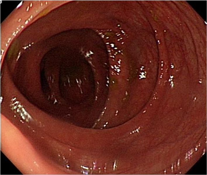
Appl. Sci. 2020, 10, 404                                                                            2 of 15

used for colonoscopy video images to label abnormal colorectal mucosa for helping gastroenterologists
to diagnose colon polyps and tumors. The paper recorded good results with a sensitivity of 90%
and specificity of 97%. The result proves that it is feasible to assist endoscopic physicians with
computer-assisted methods.
     According to research, CAD analysis of colonoscopy images has been proven to be useful, but no
studies have yet used gray-level co-occurrence matrices (GLCMs) or other texture analysis models
to analyze images obtained from patients with MC during general endoscopy nor the relationship
between mucosal image texture and pathological results in patients with MC. Therefore, this study
analyzed the pathological results of polyps of patients with MC through the texture features of general
colonoscopy images. The GLCM model can analyze image data suitably [7] and is suitable for MC
with special textures. If MC and polyps are detected during colonoscopy, the possible pathological
results can be predicted by analyzing images. The patients can be subsequently instructed to stop
using anthranoid laxative agents, and a polypectomy is scheduled for poor differentiated polyp which
means a better prognosis. [8].
     MC is a historical disease [9,10]. Cruveilhier first discovered this phenomenon in 1829, and in
1857, Virchow officially named it MC [11]. Long-term use of anthranoid laxative or of these herbs
can cause MC after 3–13 months [12], these drugs include sennoside; Normacol; the Chinese herbal
medicine containing polygonum, aloe, senna, and rhubarb; and cascara sagrada [13]. MC can be
divided into three phases according to chromaticity and texture [11]: (1) light brown colonic mucosa
with no apparent boundaries with normal mucosa, (2) dark brown colonic mucosa with clear linear
or noncontinuous boundaries with normal mucosa, and (3) dark black colonic mucosa with linear or
spotted boundaries with normal mucosa. MC often disappears after the relevant drug is stopped for
six months to one year.
     Colon polyps are epidermal protrusions in the lumen of the colon and can be roughly classified
into six categories according to the Paris classification: pedunculate, sessile, superficial and elevated,
superficial and flat, superficial and depressed, and concave [14]. In general, colorectal polyps can
be roughly divided into three categories: (1) hyperplastic polyps, (2) adenoma polyps (adenoma;
potentially divided into tubular adenoma, tubulovillous adenoma, and villous adenomas, which
is the most malignant), and (3) neoplastic polyps (including carcinoma in situ, carcinoid polyp,
and adenocarcinoma). The earlier detection of neoplastic polyps makes the treatment become more
effective [8]. Auxiliary methods can help gastroenterologists to gauge which polyps most urgently
require treatment. This can solve problems related to malignant adenoma and even colorectal cancer
in patients with MC.
     In Mainland China, MC is prominent among men aged >60 years and adenomatous polyp
hyperplasia is the most common comorbidity [2]. These patients are more prone to proliferative polyps
and adenomas [15] and to having higher adenoma detection rates (ADRs) than patients receiving
general colonoscopy [1]. MC patient are prone to polyposis; the proportion of patients in the class is
approximately 34.7% [1], whereas the corresponding proportion for the normal population is 26.5% [1].
MC prevalence during colonoscopy is 1.78% according to a 2018 Chinese study [2] and approximately
3.13% in a 1993 colonoscopy study [16]. Thus, MC may be related to colorectal cancer. In addition, MC
was observed in patients with colorectal cancer [15]. Therefore, MC is caused by the drug causing
chronic inflammation and blackening of the colon, and its relationship with carcinoembryonic antigens
(CEAs) warrants discussion.

2. Materials and Methods

2.1. Colonoscopy Database
    All collected colonoscopy images were captured with the general colonoscopes produced by
Olympus Corporation of Japan (Shinjuku Monolith, 2-3-1 Nishi-Shinjuku, Shinjuku-ku, Tokyo 163-0914,
Japan). Colonoscopes models were GF-260 and 290, so we can ensure that the image quality were close.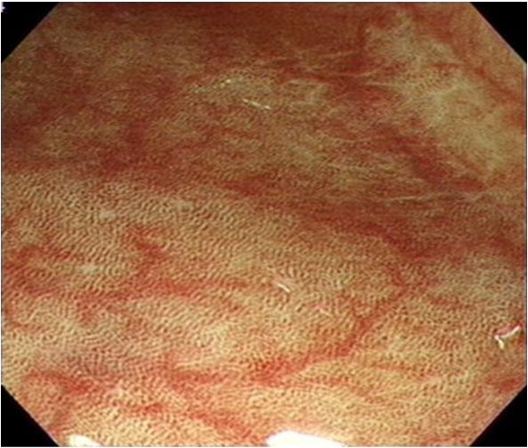
Appl. Sci. 2020, 10, 404                                                                             3 of 15

Endoscopic images were obtained by gastroenterologists from Taipei Medical University Hospital,
Taipei, Taiwan.
      A small amount of patient data was used for analysis, and decided the next method of analyzing
pictures and data for the research. We analyzed data of 298 patients with MC from the database
between 1 January 2016 and 17 July 2017; In the initial analysis of the study, the analysis of polyp
texture in patients without tumor index such as CEAs or CA 199 was not related to pathological
findings, so we included only 124 patients who had CEA data and clear colonoscopy images. We then
analyzed these patients’ colonoscopy images. The 124 patients’ images survey indicated that if analysis
is conducted using a large size image or if the reflection of feces are not avoided and the part with
white text recorded in the image is not removed, it may be caused by the aforementioned interference.
This can lead to unsatisfactory results. Regarding the usefulness of correcting images according
to patients’ normal skin and luminosity, because the calculation results are based on the gray-level
symbiotic matrix analysis method, the final calculated result exerted little effect. The patient’s normal
skin and brightness were therefore not ultimately required for correction. We also observed that taking
a polyp image consisting of 100 × 100-pixel squares from the center point provided improved texture
features and results.
      Next, 51,891 colonoscopy data were acquired from the Division of Gastroenterology and
Hepatology, Department of Internal Medicine, Taipei Medical University Hospital. The research
encompassed the period from 1 January 2012 to 30 September 2017. The research materials and
images were deidentified by the Taipei Medical University Human Research Joint Ethics Committee for
research permission and ensured that research materials and images were deidentified. No informed
consent is required for this retrospective study. After the adoption, relevant research and statistical
work was commenced. Among them, 28,974 colonoscopy data had polyps; thus, the polyp detection
rate (PDR) was 55.84%. Because 12,244 times colonoscopy data presented with adenoma or colorectal
cancer, adenoma detection rate (ADR) was 23.60%. Finally, 834 patients presented with colorectal
cancer, so the detection rate of colorectal cancer was 1.61%.
      Next, from these data, the total number of patients with a diagnosis of MC was observed to
be 1092, and the MC prevalence rate was 2.1%, similar to the prevalence rate of 1.78% in Mainland
China [2]. These patients included 787 women and 305 men, and therefore, the women had an
incidence of MC 2.58 times that of men. The age distribution of these patients was as young as 17
and as large as 97. Of these, 96 patients were over 80 years old, and 480 patients were between 60
and 80 years old. Only three patients were younger than 20. The first patient received colonoscopy
study on 2 January 2012. The last patient underwent a colonoscopy on 29 September 2017. Among
these patients, 658 patients had polyps. 390 patients had colon adenoma detected by colonoscopy.
18 patients’ pathology reports had colon cancer.
      Based on the data collected from 1092 person-times, the PDR and ADR were 60.26% and 35.71%,
respectively—close to the 34.7% noted in other studies [1]. Colorectal cancer detection rate was 1.65%.
Compared with data from the previous database, patients with MC had a slightly higher PDR than did
patients who had received general colonoscopy (4.42%); moreover, the ADR was much higher (12.11%),
and the colorectal cancer detection rate was similar. The result indicating that patients with MC were more
prone to adenoma corresponds with results reported previously [1] and indicates that even if patients
with MC are more likely to exhibit polyps under colonoscopy, they have a higher adenoma incidence than
other people do. MC is associated with adenomas. The study initially used a smaller quantity of data and
image analysis to help determine the pattern of screening and analysis for all subsequent data.
      We excluded the data of patients without CEAs, poor colon preparation, or with unclear data.
Finally, 370 patients were included in the image analysis study. The relationship between image texture
GLCMs and CEAs was compared. Among the 370 patients, 181 had polyps and pathological biopsies.
The study used images of 181 patients. All pictures collected by one gastroenterologist. Using Image
J, a 100 × 100-pixel block diagram—taken from outside areas where feces had accumulated or from
positions in the centers of polyps—was isolated for analysis. Images were divided into three groups: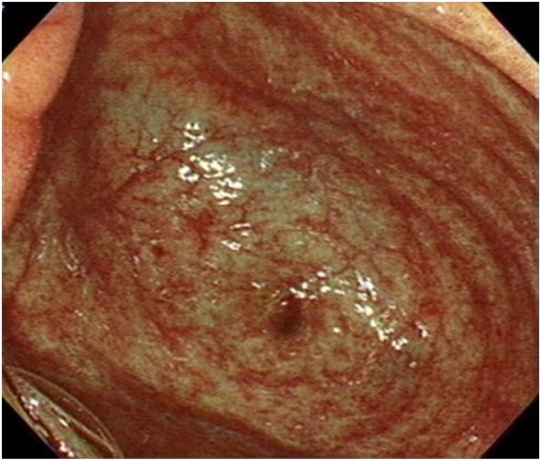
Appl. Sci. 2020, 10, 404 4 of 15
1. Cecem, image of the appendix and cecal mucosa (C), consisting of 181 images.
2. Splenic flexure spleen images (S), consisting of 181 images.
Appl. Sci. 2020, 10, x FOR PEER REVIEW 4 of 15
3. Appl.
Polyp (P), 10,
Sci. 2020, if the
x FORpatient had a polyp or a tumor. If multiple polyps were present, we
PEER REVIEW collected
4 of 15
3. thePolyplargest
(P), ifand
themost prominent
patient textured
had a polyp polyp.
or a tumor. The gastroenterologist
If multiple manually
polyps were present, cut the image
we collected
3.from Polyp
central(P),point
if the of
patient had a polyp
the polyp. or a resulted
This also tumor. If inmultiple polypsFigure
181 images. were present,
1a showswe collected
the largest and most prominent textured polyp. The gastroenterologist manually cut the one
imagemelanosis
the largest and most prominent textured polyp. The gastroenterologist manually cut the image
coli
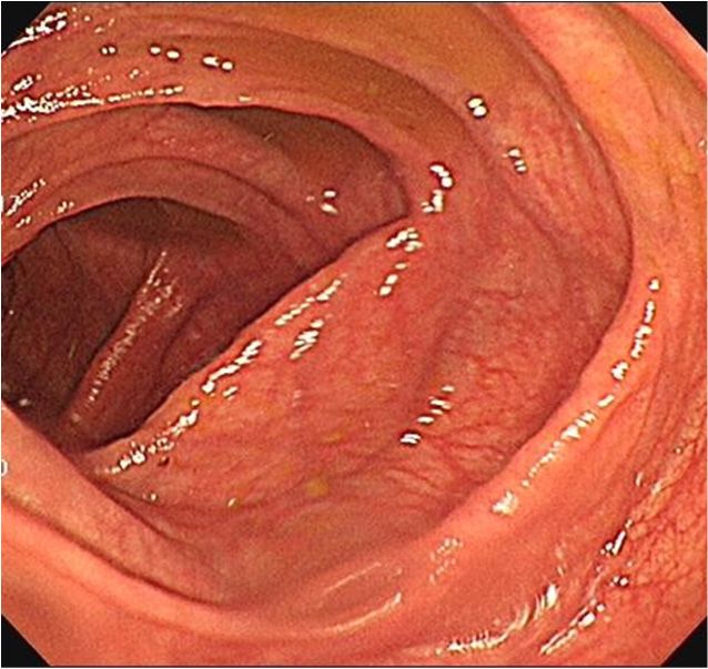
from central point of the polyp. This also resulted in 181 images. Figure 1a shows one melanosisstopping
patient’s cecal image and Figure 1b shows the same patient’s cecal image after
from central point of the polyp. This also resulted in 181 images. Figure 1a shows one melanosis
coli patient’s cecal
anthraquinone image and
containing Figureagents
laxative 1b showsfor the
six same patient’s cecal image after stopping
months.
coli patient’s cecal image and Figure 1b shows the same patient’s cecal image after stopping
anthraquinone containing laxative agents for six months.
anthraquinone containing laxative agents for six months.
(a) (b)
(a) (b)
Figure
Figure1. Melanosis
1. Melanosis colicoli patient’s
patient’s cecal images.
cecal images. (a) The
(a) The patient tookpatient took anthraquinone
anthraquinone containing
containing laxative
Figure 1. Melanosis coli patient’s cecal images. (a) The patient took anthraquinone containing laxative
laxative
medicinemedicine
one year one
and year and his colonoscopy
his colonoscopy image
image revealed revealed
blackish blackish
mucosal mucosal
pattern in colon.pattern
(b) The in colon.
medicine one year and his colonoscopy image revealed blackish mucosal pattern in colon. (b) The
(b) Thepatient’s
same same patient’s
cecal imagececal image
after after six
six months. months.
Blackish Blackish
mucosal mucosal
pattern pattern
disappeared afterdisappeared
stopping after
same patient’s cecal image after six months. Blackish mucosal pattern disappeared after stopping
anthraquinone
stopping containingcontaining
anthraquinone laxative agent for 6 months.
laxative agent for 6 months.
anthraquinone containing laxative agent for 6 months.
Thissection
This sectiondescribes
describes the
the image
image analysis
analysis methods
methods used ininthis study, like this article [17]. TheThe way
This section describes the image analysis methodsused
used inthis
thisstudy,
study,like
like this
this article [17].
article [17]. The
weway
use we use computer
computer programs
programs to to analyze
analyze textures
textures has has been
also also been
widely widely
used used
in in other
way we use computer programs to analyze textures has also been widely used in other areasThe
other areasareas
[18]. [18]. images
[18].
The images
are divided are
intodivided into three groups as previously described. Example images of patients with
The images arethree groups
divided as previously
into three described.described.
groups as previously Example imagesimages
Example of patients with
of patients MC are
with
MC are illustrated in Figure 2a–c and the examples of regions of interest in Figure 2d–f.
illustrated
MC arein Figure 2a–c
illustrated and the
in Figure 2a–cexamples of regions
and the examples of interest
of regions in Figure
of interest 2d–f.2d–f.
in Figure
(a) (b) (c)
(a) (b) (c)
(d) (e) (f)
(d) (e) (f)
Figure 2. Images extracted from one patient with melanosis coli (a) cecum, (b) splenic flexure, and (c)
FigureImages
2. Images extractedfrom
from one
one patient with melanosis coli coli
(a) cecum, (b) splenic flexure, flexure,
and (c) and
Figure polyp. The extracted
colon 2. regions of interest (d)patient with
cecum—from melanosis
(a); (e) splenic (a) cecum,
flexure—from (b) (b);
splenic
(f) colon
colon polyp.
(c)polyp—from
colon polyp. The regions of interest (d) cecum—from (a); (e) splenic flexure—from (b); (f) colon
(c). The regions of interest (d) cecum—from (a); (e) splenic flexure—from (b); (f) colon
polyp—from (c).
polyp—from (c).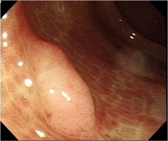
Appl.
Appl. Sci.
      Sci. 2020,
           2020, 10,
                 10, x404
                       FOR PEER REVIEW                                                                                           5 5of
                                                                                                                                     of 15
                                                                                                                                        15

     The images demonstrate that the MC has a particular dark brown pigmentation and presents a
     The
special    images
        black       demonstrate
               texture;              that the
                         places without       MC has a particular
                                            pigmentation             dark
                                                            are white.  Thebrown   pigmentation
                                                                             color textures         and or
                                                                                             of polyps     presents
                                                                                                              tumorsa
special black  texture; places  without    pigmentation   are white.  The  color textures of polyps
are obviously different from the surroundings, exhibiting lighter and more turbulent textures, and    or  tumors  are
obviously
most        different
      of them         from
                have no      the texture.
                          black   surroundings, exhibiting lighter and more turbulent textures, and most of
themWe have  no  black texture.
          analyze the GLCM for quantitative feature extraction and the 14 features of the GLCM. The
     We analyze
characteristics  of the study
                         GLCMare    fordivided
                                        quantitative   feature
                                                 into three     extraction
                                                             types: pattern,and   the 14 features
                                                                              brightness,            of thefeatures.
                                                                                            and texture       GLCM.
The characteristics
Analysis              of theon
          focuses mainly      study   are divided
                                 the texture        into three
                                              features,        types:
                                                         and the      pattern,
                                                                  results       brightness,
                                                                          are calculated      andthe
                                                                                          using    texture   features.
                                                                                                       colonoscopy
Analysis   focuses  mainly   on  the  texture  features, and  the results are calculated  using   the
image RGB channels. The method for verifying the results uses the Pearson correlation coefficient to   colonoscopy
image the
verify  RGBcorrelation
              channels. between
                           The method      for verifying
                                       features           the resultsresults.
                                                  and pathological     uses the  Pearson
                                                                               The         correlation
                                                                                    tool calculates    thecoefficient
                                                                                                             Pearson
to verify thecoefficients
correlation    correlationandbetween     features
                                   p values   usingandMSpathological
                                                           Excel and results.   The toolPackage
                                                                       IBM Statistical    calculates forthe
                                                                                                          thePearson
                                                                                                               Social
correlation  coefficients  and  p  values  using  MS  Excel and  IBM  Statistical Package   for the Social
Sciences (SPSS). A Pearson correlation coefficient close to 0.4 and a p of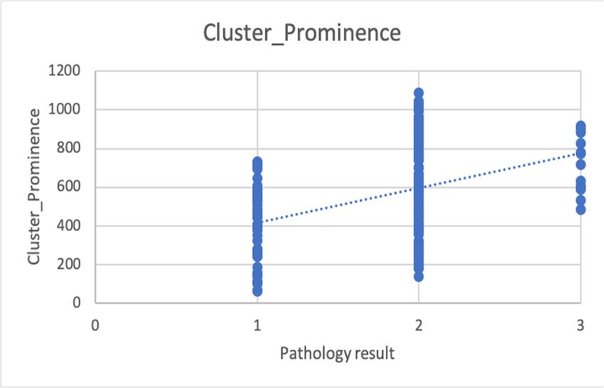
Appl. Sci. 2020, 10, 404                                                                              6 of 15

of computed tomography to simulate colonoscopy for polyp detection has also been studied [24].
In addition, one study analyzed pathological biopsies for colorectal cancer and normal colorectal
mucosa [25], and this technique can provide clinicians with valuable assistance. Because this represents
the earliest and the most mature image texture analysis method, this study analyzes the colorectal polyp
image texture characteristics of patients with MC. The GLCM has a total of 14 features: autocorrelation,
dissimilarity, energy, entropy, homogeneity, difference variance, difference entropy, information
measure of correlation, inverse difference normalized, inverse difference moment, cluster prominence,
cluster shade, contrast, and correlation. These features can be clinically applied to the analysis of
various images. For the analysis of medical images, the features are employed mainly to study
their correlations with various lesions. Of the 14 features analyzed in this study, only eight were
related to the final results: entropy, energy, correlation, dissimilarity, homogeneity, autocorrelation,
cluster_prominence, and cluster_shade.
       Entropy is a measure of the quantity of information that an image possesses. Texture information
also qualifies as image information. It is a measure of randomness. When all elements in the
co-occurrence matrix possess maximum randomness and all values in the spatial co-occurrence matrix
are almost equal, the elements in the co-occurrence matrix are dispersed, and the entropy (fluctuation)
is large. This represents the degree of nonuniformity or complexity of the texture in the image.
       Energy refers to the sum of the squares of the values of the GLCM elements, so it is also called
energy. This reflects the uniformity of the gray scale distribution of the image and the texture thickness.
If all values of the co-occurrence matrix are equal, the angular second moment (ASM) energy value is
small; conversely, if some of the values are large and other values are small, the ASM energy is high.
When the elements in the symbiotic matrix are concentrated, the ASM energy is high. Higher ASM
energy indicates more uniform and regularly varying texture pattern.
       Correlation is used to distinguish whether two objects have mutual correlations in shape and
other features, and then, the correlation value is used to determine the characteristics of the object
to locate the object. CorrelationM indicates the gray-level linear correlation between a pixel and its
neighbors, similar to Correlation.
       Dissimilarity is the degree of dissimilarity in gray-level value measurements for an image. It is
sensitive to the arrangement of gray-level values in space or the hue of the image.
       Homogeneity is used to reflect the homogeneity of image textures and to measure how much
image texture changes locally. A large value indicates a lack of variation between different regions of
the image texture, and the locality is largely uniform.
       Autocorrelation is the degree of similarity of the metric spatial GLCM elements in the row or
column direction. Therefore, the correlation value reflects the local grayscale correlation in the image.
When the matrix element values are similar, the correlation value is large; conversely, if the matrix
cell values differ greatly, the correlation value is small. If the image has a horizontal direction texture,
the correlation value of the horizontal direction matrix is greater than the correlation value of the
remaining matrix. The more vicious the image of the polyp, the higher the value of the relationship for
horizontal or vertical textures is.
       Cluster_prominence and cluster_shade indicate a lack of symmetry in the gray-level distribution.
Therefore, the more malignant a polyp, the more complex is the polyp texture and the
surrounding asymmetry.
       In this study, the gastroenterologist manually used a 100 × 100-pixel box to mark the polyps then
extracted and quantified the brightness features and texture features and analyzed the GLCM features
of the colonoscopy images to obtain some of the MC. If the final pathological results confirm that
texture features demonstrate Pearson correlation with pathological results, this model can be used as a
reference for clinicians. As long as a gastroenterologist performs a colonoscopy, polyps that may be
poorly pathologically differentiated can be treated immediately.

                                                  X X
                            Autocorrelation =                     px − µx py − µy /σx σy                 (1)
                                                     i    j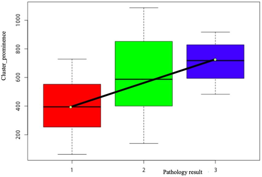
Appl. Sci. 2020, 10, 404                                                                                                                                       7 of 15

                                                  X                    X X
                                Contrast =                        n2                                       p(i, j) , i − j = n                                    (2)
                                                              n                    i                   j
                                                                  P P
                                                                       i       j ( i − µx )                            j − µy p(i, j)
                                    Correlation =                                                                                                                 (3)
                                                     σx σy
                                                 X X                4
                            Cluster prominence =      i + j − µx − µy p(i, j)                                                                                     (4)
                                                                               i                   j
                                                                  X X                                        4
                              Cluster shading =                                                i + j − µx − µy p(i, j)                                            (5)
                                                                           i           j
                                                                               X X
                                         Dissimilarity =                                                           p(i, j) i − j                                  (6)
                                                                                           i                   j
                                                                           X X
                                              Energy =                                                         p(i, j)2                                           (7)
                                                                                   i                   j
                                                                  X X
                                     Entropy = −                                           p(i, j) log(p(i, j))                                                   (8)
                                                                           i           j

                                                                  1            X X
                                    Homogeneity = −                    p(i, j)                                                                                    (9)
                                                             1+i−j                     i                   j
                                                           X
                                    Difference variance =       i2 px−y (i)                                                                                     (10)
                                                              i
                                                      X
                              Difference entropy = −      px+y (i) log px+y (i)                                                                                 (11)
                                                                                               i

                                          HXY−HXY1                       P P
    Information measure of correlation = max{HX,HY}   HXY = (8) HXY1 = − i j p(i, j) log px (i)py (j) HX =
                                                                                                                                                                (12)
                                      entropy of px , HY = entropy of py
                                                                                                       X X                                  1
                           Inverse difference normalized =                                                                                           p(i, j)    (13)
                                                                                                                       i           j   1+ i−j
                                                                                           X X                                          1
                           Inverse difference moment =                                                                                              p(i, j)     (14)
                                                                                                           i               j
                                                                                                                               1 + (i − j)2
where µx , µy , σx , and σy are the mean and standard deviation (SD) of the marginal distributions
of p(i,j|d,θ);                       X X                  X X
                                µx =    i   p(i, j), µy =  j   p(i, j)                         (15)
                                              i       j                                                            j           i
                                    X                 X                                                    X                           2 X
                            σ2x =        (i − ux )2               p(i, j), σ2y =                                           j − uy                   p(i, j)     (16)
                                     i                    j                                                        j                            i

3. Results
      Because some data came from the same patients at different ages, the age of the first discovery
was taken as the patient’s MC age. After removing duplicate patient medical records, we had 938
patients with MC diagnosed through colonoscopy in our hospital within six years; 694 (74%) were
female and 244 (26%) male. The incidence of female patients after correction was 2.84 times higher
than that of male patients. In total, 11 (1.2%), 341 (36.3%), 447 (47.7%), and 139 (14.8%) patients were
aged 76 years, respectively. Therefore, age wise, the most MC-affected of
patient group was of those aged >51 years; 62.5% of them were. Older patients were more likely to
experience constipation. These patients are more likely to be affected by MC following anthranoid
laxative use.
      Among the 938 patients, 438 patients had CEA data. The CEA cutoff point was 4.7 ng/mL.
Sixty-two people with CEAs exceeded the cutoff point, and compared the relationship between image
texture GLCM and CEAs. After unclear and unsuitable patient data were excluded, 370 patients were
finally analyzed.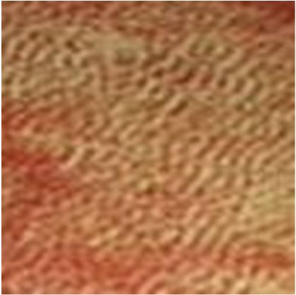
Appl. Sci. 2020, 10, 404                                                                                         8 of 15

     First, the correlation between CEAs and MC mucosal texture was analyzed. For example,
Pearson correlation between autocorrelation and CEAs was −0.005993648. Pearson correlation between
contrast and CEAs was −0.045998786. Finally, no correlation occurred between CEAs and the texture
characteristics of MC mucosa.
     Among the 370 patients, 181 patients had polyps and pathological results, and the differentiative
degree of polyps belonged to 130 of the adenomatous polyps. The ADR was 35.14% in 370 patients with
MC. This result was similar to the 35.88% ADR for all 1092 individuals. Patients with MC exhibited
an ADR similar to 34.7% cited by other studies in mainland China [1,26]. This also indicates that the
presence or absence of CEA detection is not directly related to ADR in patients with MC, but patients
with MC have a higher ADR than the general population does.
     All the images were then analyzed using the GLCM for texture features. Because these 181 patients
had polyps, each one had three type images for analysis. In total, 543 images were obtained. Table 1
presents the 181 patients’ data and the SPSS calculations and statistics.

          Table 1. Association between carcinoembryonic antigens (CEAs) and GLCMs texture features.

     Correlation (Number = 181)              Correlation-M         Correlation      Dissimilarity        Energy
                             Pearson             0.094                0.094            −0.073            0.001
       CEAs
                            Two-tailed
                                                 0.210                0.210             0.331            0.991
                           significance
      Correlation (number = 181)                Entropy          Homogeneity-M      Homogeneity
                             Pearson            −0.068                0.088             0.087              -
       CEAs
                            Two-tailed
                                                 0.361                0.237             0.244
                           significance

     Continuing to count the polyp pathological results, we observed that the texture features and
the classification of pathological results were related for certain characteristics. As discussed in other
research, the pathological results of polyps in patients with MC are classified into three grades according
to their benign and malignant degrees: The first grade includes benign hyperplastic polyp, Hamartoma
polyp, pseudopolyps, and inflammatory polyps. The second involves adenomas, including tubular
adenomas, tubulovillous adenomas, and villous adenomas. The third grade includes adenocarcinomas,
along with both carcinoids and carcinomas in situ. If patients with MC have malignant colorectal
adenocarcinomas, the textures of the endoscopy images are extremely disordered. The Pearson
correlation coefficient between features and polyp grades was calculated.
     First, the SPSS calculation demonstrated that the Pearson correlation coefficient was 0.390
(p < 0.001) for autocorrelation (Tables 2 and 3). It is illustrated in Figures 4 and 5.

                             Table 2. Association of autocorrelation with pathological grade.

                                            Correlation                              Autocorrelation
                                                           Pearson correlation             0.390
                   Polyp pathological grade (1–3)         Two-tailed significance        p < 0.001
                                                                 Number                     181

                           Table 3. Association of cluster_prominence with pathological grade.

                                          Correlation                               Cluster_Prominence
                                                         Pearson correlation               0.398
               Polyp pathological grade (1–3)           Two-tailed significance          p < 0.001
                                                               Number                       181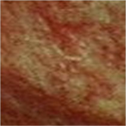
Appl. Sci. 2020, 10, 404                                                                               9 of 15
Appl. Sci. 2020, 10, x FOR PEER REVIEW                                                                9 of 15

                                                    (a)

                                                    (b)
     Figure 4. The correlations between autocorrelation and pathological results (a) scatter plot and
     Figure 4. The correlations between autocorrelation and pathological results (a) scatter plot and (b)
     (b) box-and-whisker plot. Pathology result 1 is hyperplastic polyps. Pathology result 2 is adenoma.
     box-and-whisker plot. Pathology result 1 is hyperplastic polyps. Pathology result 2 is adenoma.
     Pathology result 3 is colon adenocarcinoma.
     Pathology result 3 is colon adenocarcinoma.

     For cluster_prominence and cluster_shade, the Pearson correlation coefficient was 0.398 (p ≤
0.001; Table 3, Figure 5) and 0.396 (slightly linear; p value ≤ 0.001; Table 4 and Figure 6) respectively.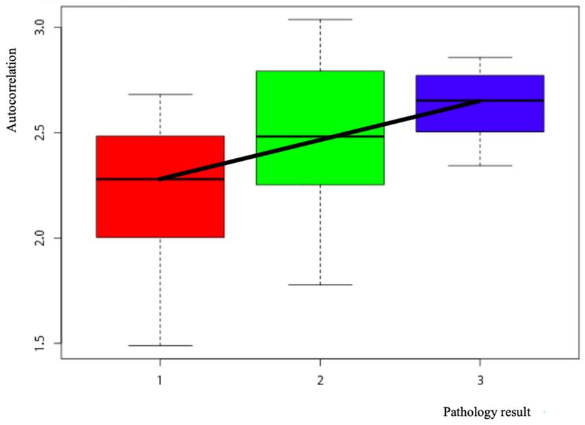
Appl. Sci. 2020, 10, 404                                                                               10 of 15
Appl. Sci. 2020, 10, x FOR PEER REVIEW                                                               10 of 15

                                                    (a)

                                                    (b)
      Figure 5. The correlations between cluster_prominence and pathological results (a) scatter plot and
     Figure 5. The correlations between cluster_prominence and pathological results (a) scatter plot and
      (b) box-and-whisker plot. Pathology result 1 is hyperplastic polyps. Pathology result 2 is adenoma.
     (b) box-and-whisker plot. Pathology result 1 is hyperplastic polyps. Pathology result 2 is adenoma.
      Pathology result 3 is colon adenocarcinoma.
     Pathology result 3 is colon adenocarcinoma.
     For cluster_prominence and cluster_shade, the Pearson correlation coefficient was 0.398 (p ≤ 0.001;
Table 3, Figure 5) and 0.396 (slightly linear; p value ≤ 0.001; Table 4 and Figure 6) respectively.
Appl. Sci. 2020, 10, x FOR PEER REVIEW 11 of 15
Appl. Sci. 2020, 10, 404 11 of 15
Table 4. Association of cluster_shade with pathological grade.
Correlation Cluster_shade
Table 4. Association of cluster_shade with pathological grade.
Pearson correlation 0.396
Correlation Cluster_Shade
Two-tailed
Polyp pathological grade (1–3) Pearson correlation 0.000, p < 0.05
0.396
Polyp pathological grade (1–3) significance
Two-tailed significance 0.000, p < 0.05
Number
Number 181
181
(a)
(b)
Figure 6. The correlations between cluster_shade and pathological results (a) scatter plot and
Figure 6. The correlations between cluster_shade and pathological results (a) scatter plot and (b) box-
(b) box-and-whisker plot. Pathology result 1 is hyperplastic polyps. Pathology result 2 is adenoma.
and-whisker plot. Pathology result 1 is hyperplastic polyps. Pathology result 2 is adenoma. Pathology
Pathology result 3 is colon adenocarcinoma.
result 3 is colon adenocarcinoma.Appl. Sci. 2020, 10, 404 12 of 15
Finally, Table 5 presents SPSS results for total Pearson correlation between all GLCM features.
Table 5. All GLCM features and pathology correlation.
Correlation Number = 181 Autocorrelation Cluster_Prominence Cluster_Shade
Pearson correlation 0.390 0.398 0.396
Polyp pathological
grade (1–3) Two-tailed
p < 0.001 p < 0.001 p < 0.001
significance
The features more related to the pathology result of polyps are autocorrelation, cluster_prominence,
cluster_shade, and so on. These features can be considered for colonoscopic examinations, when MC
and polyps are discovered, first for the gastroenterologist to predict possible pathological results.
Other features are furthermore weakly related to the pathological results, but the Pearson
correlations are small. The p values areAppl. Sci. 2020, 10, 404 13 of 15
cluster_prominence, and cluster_shade; other features such as contrast, correlationM, correlation, and
difference_variance also possess a certain degree of relevance. The five aforementioned texture features
should be applicable to clinical colonoscopy image analysis.
No evidence currently suggests that MC is directly related to malignancies. But MC is related to
adenoma [1] and adenoma is related to colorectal cancer [27]. To establish whether tumor markers
(such as CEAs, CA199, CA125, AFP, or CA724) are related to texture features after calculation may
require more data and image analysis studies. MC images require much clinical analysis, and the
results should be provided for gastroenterologists prescribing relevant laxatives, mainly because MC is
a reversible condition. For instance, if a patient who has MC with polyps exhibits particular textures or
colon mucosal changes under colonoscopy, doctors can terminate the use of the relevant medication
and prescribe different laxatives instead.
In addition, contrast mode reflects the clarity of the image and the degree of texture groove
depth. The previous study did not mention that longer use of a relevant drug caused darker contrast.
More data collection may confirm more correlations. Therefore, the longer drugs potentially able to
affect colon mucosa coloring are used, the more obvious the texture. The effects of intestinal bacteria
can be further analyzed in the future. In addition to GLCMs, other texture analysis methods such as
gray-level run length matrix (16 features), gray-level size zone matrix (16 features), neighboring gray
tone difference matrix (5 features), and gray-level dependence matrix (14 features) should be attempted.
If these methods can be used to analyze polyp texture, new knowledge and understanding may be
achieved. These quantitative image textures can also be combined in evaluating tumor malignancy or
cancer types in the future using machine learning-based systems.
Some endoscopy studies have applied computer-assisted diagnostic analysis, such as capsule
endoscopy, after capturing images of the intestines. The computer analysis of capsule endoscopes
often entails use of MATLAB, mainly employing the red (R) channel primarily to capture red bleeding
points or bleeding lesions [28]. However, colors other than red, such as black, green, and brown, are
rarely included in the search. Therefore, the analysis of mucosal images and polyps under endoscopy
is valuable [29]. The results of this study of MC suggest that in the future, endoscopy or colon-capsule
endoscopy can provide clinical assistance in MC and polyp detection.
5. Conclusions
MC polyp texture was related to the pathological results of GLCM feature analysis, especially in
the three features (autocorrelation, cluster_prominence, cluster_shade). In the future, photographs of
the polyps taken during colonoscopy may potentially be used to detect colon MC and polyps and the
five features for analysis employed to help gastroenterologists predict the possible pathological results
for polyps in advance. This can save the patients’ lives.
If this model can be developed, in the future, endoscopy doctors will be able to analyze uploaded
colonoscopy images on a computer and establish the correlation between the texture features of
different colorectal mucosa and clinical indicators, or even pathological results, then predict possible
outcomes. In addition to colonoscopy, similar characterization methods should be applicable to other
endoscopic imagery such as capsule endoscopic images. In short, this approach should be extensively
applied in the future. This method effectively improves the efficiency of the examination and saves
time, which is helpful for clinicians. This result should be used in the future to design an instant help
software to help the gastroenterologist.
Author Contributions: Conceptualization, C.-M.L.; data curation, C.-M.L.; methodology, C.-M.L.; validation,
C.-M.L.; writing—original draft, C.-M.L.; writing—review and editing, H.-J.Y.; investigation, H.-J.Y.; visualization,
H.-J.Y.; supervision, C.-C.C. (Chun-Chang Chen); resource, C.-C.C. (Chun-Chao Chang); software, Y.-H.Y.
All authors have read and agreed to the published version of the manuscript.
Funding: This research received no external funding.Appl. Sci. 2020, 10, 404 14 of 15
Acknowledgments: The authors would like to thank the Division of Gastroenterology and Hepatology, Department
of Internal Medicine, Taipei Medical University Hospital for financially supporting this research. This manuscript
was edited by Wallace Academic Editor to assist with English grammar correction.
Conflicts of Interest: The authors declare no conflict of interest.
References
1. Blackett, J.W.; Rosenberg, R.; Mahadev, S.; Green, P.H.R.; Lebwohl, B. Adenoma Detection is Increased in the
Setting of Melanosis Coli. J. Clin. Gastroenterol. 2018, 52, 313–318. [CrossRef] [PubMed]
2. Wang, S.; Wang, Z.; Peng, L.; Zhang, X.; Li, J.; Yang, Y.; Hu, B.; Ning, S.; Zhang, B.; Han, J.; et al. Gender, age,
and concomitant diseases of melanosis coli in China: A multicenter study of 6,090 cases. PeerJ 2018, 6, e4483.
[CrossRef] [PubMed]
3. Cowley, K.; Jennings, H.W.; Passarella, M. Who Turned Out the Lights? An Impressive Case of Melanosis
Coli. ACG Case Rep. J. 2015, 3, 13–14. [CrossRef] [PubMed]
4. Zhou, X.; Wang, P.; Zhang, Y.J.; Xu, J.J.; Zhang, L.M.; Zhu, L.; Xu, L.P.; Liu, X.M.; Su, H.H. Comparative
proteomic analysis of melanosis coli with colon cancer. Oncol. Rep. 2016, 36, 3700–3706. [CrossRef]
5. Yoshida, H.; Nappi, J.; MacEneaney, P.; Rubin, D.T.; Dachman, A.H. Computer-aided diagnosis scheme for
detection of polyps at CT colonography. Radiographics 2002, 22, 963–979. [CrossRef]
6. Karkanis, S.A.; Iakovidis, D.K.; Maroulis, D.E.; Karras, D.A.; Tzivras, M. Computer-aided tumor detection in
endoscopic video using color wavelet features. IEEE Trans. Inf. Technol. Biomed. 2003, 7, 141–152. [CrossRef]
7. Chang, C.C.; Chen, H.H.; Chang, Y.C.; Yang, M.Y.; Lo, C.M.; Ko, W.C.; Lee, Y.F.; Liu, K.L.; Chang, R.F.
Computer-aided diagnosis of liver tumors on computed tomography images. Comput. Methods Programs
Biomed. 2017, 145, 45–51. [CrossRef]
8. Zauber, A.G.; Winawer, S.J.; O’Brien, M.J.; Lansdorp-Vogelaar, I.; van Ballegooijen, M.; Hankey, B.F.; Shi, W.;
Bond, J.H.; Schapiro, M.; Panish, J.F.; et al. Colonoscopic polypectomy and long-term prevention of
colorectal-cancer deaths. N. Engl. J. Med. 2012, 366, 687–696. [CrossRef]
9. Walker, N.I.; Bennett, R.E.; Axelsen, R.A. Melanosis coli. A consequence of anthraquinone-induced apoptosis
of colonic epithelial cells. Am. J. Pathol. 1988, 131, 465–476.
10. Byers, R.J.; Marsh, P.; Parkinson, D.; Haboubi, N.Y. Melanosis coli is associated with an increase in colonic
epithelial apoptosis and not with laxative use. Histopathology 1997, 30, 160–164. [CrossRef]
11. Liu, Z.H.; Foo, D.C.C.; Law, W.L.; Chan, F.S.Y.; Fan, J.K.M.; Peng, J.S. Melanosis coli: Harmless pigmentation?
A case-control retrospective study of 657 cases. PLoS ONE 2017, 12, e0186668. [CrossRef] [PubMed]
12. Mellouki, I.; Meyiz, H. Melanosis coli: A rarity in digestive endoscopy. Pan Afr. Med. J. 2013, 16, 86.
[CrossRef] [PubMed]
13. Modi, R.M.; Hussan, H. Melanosis Coli After Long-Term Ingestion of Cape Aloe. ACG Case Rep. J. 2016, 3,
e157. [CrossRef] [PubMed]
14. The Paris endoscopic classification of superficial neoplastic lesions: Esophagus, stomach, and colon:
November 30 to December 1, 2002. Gastrointest. Endosc. 2003, 58, S3–S43. [CrossRef]
15. Biernacka-Wawrzonek, D.; Stepka, M.; Tomaszewska, A.; Ehrmann-Josko, A.; Chojnowska, N.; Zemlak, M.;
Muszynski, J. Melanosis coli in patients with colon cancer. Prz. Gastroenterol. 2017, 12, 22–27. [CrossRef]
16. Siegers, C.P.; von Hertzberg-Lottin, E.; Otte, M.; Schneider, B. Anthranoid laxative abuse-a risk for colorectal
cancer? Gut 1993, 34, 1099–1101. [CrossRef]
17. Chung-Ming Lo, P.-H.H.; Kevin Li-Chun, H. Computer-Aided Detection of Hyperacute Stroke Based on
Relative Radiomic Patterns in Computed Tomography. Appl. Sci. 2019, 9, 1668. [CrossRef]
18. Chang, R.F.; Lee, C.C.; Lo, C.M. Quantitative diagnosis of rotator cuff tears based on sonographic pattern
recognition. PLoS ONE 2019, 14, e0212741. [CrossRef]
19. Haralick, R.; Shanmugam, K.; Dinstein, I. Textural Features for Image Classification. IEEE Trans. Syst.
Man Cybern. 1973, 3, 610–621. [CrossRef]
20. Haralick, R. Statistical and structural approaches to texture. Proc. IEEE 1979, 67, 786–804. [CrossRef]
21. Vadakkenveettil, B.S.; Unnikrishnan, A.; Balakrishnan, K. Grey Level Co-Occurrence Matrices: Generalisation
and Some New Features. Int. J. Comput. Sci. Eng. Inf. Technol. 2012, 2, 151–157. [CrossRef]Appl. Sci. 2020, 10, 404 15 of 15
22. Alvarenga, A.V.; Pereira, W.C.; Infantosi, A.F.; Azevedo, C.M. Complexity curve and grey level co-occurrence
matrix in the texture evaluation of breast tumor on ultrasound images. Med. Phys. 2007, 34, 379–387.
[CrossRef] [PubMed]
23. Rahebi, J.; Hardalac, F. Retinal blood vessel segmentation with neural network by using gray-level
co-occurrence matrix-based features. J. Med. Syst. 2014, 38, 85. [CrossRef] [PubMed]
24. Summers, R.M. Challenges for computer-aided diagnosis for CT colonography. Abdom Imaging 2002, 27,
268–274. [CrossRef] [PubMed]
25. Stefanescu, D.; Streba, C.; Cartana, E.T.; Saftoiu, A.; Gruionu, G.; Gruionu, L.G. Computer Aided Diagnosis
for Confocal Laser Endomicroscopy in Advanced Colorectal Adenocarcinoma. PLoS ONE 2016, 11, e0154863.
[CrossRef] [PubMed]
26. Dik, V.K.; Moons, L.M.; Siersema, P.D. Endoscopic innovations to increase the adenoma detection rate during
colonoscopy. World J. Gastroenterol. 2014, 20, 2200–2211. [CrossRef] [PubMed]
27. Tezuka, F.; Chiba, R.; Iwama, N.; Takahashi, T. Development of the human colonic adenocarcinoma from
adenoma as a histopathologically continuous process. Tohoku J. Exp. Med. 1992, 168, 257–263. [CrossRef]
28. Kundu, A.K.; Fattah, S.A.; Rizve, M.N. An Automatic Bleeding Frame and Region Detection Scheme for
Wireless Capsule Endoscopy Videos Based on Interplane Intensity Variation Profile in Normalized RGB
Color Space. J. Healthc. Eng. 2018, 2018, 9423062. [CrossRef]
29. Sun, X.; Dong, T.; Bi, Y.; Min, M.; Shen, W.; Xu, Y.; Liu, Y. Linked color imaging application for improving the
endoscopic diagnosis accuracy: A pilot study. Sci. Rep. 2016, 6, 33473. [CrossRef]
© 2020 by the authors. Licensee MDPI, Basel, Switzerland. This article is an open access
article distributed under the terms and conditions of the Creative Commons Attribution
(CC BY) license (http://creativecommons.org/licenses/by/4.0/).You can also read