Face Alignment through Subspace Constrained Mean-Shifts
←
→
Page content transcription
If your browser does not render page correctly, please read the page content below
Face Alignment through Subspace Constrained Mean-Shifts

                                  Jason M. Saragih, Simon Lucey, Jeffrey F. Cohn
                                 The Robotics Institute, Carnegie Mellon University
                                            Pittsburgh, PA 15213, USA
                                       {jsaragih,slucey,jeffcohn}@cs.cmu.edu

                         Abstract                                 detection ambiguities as a direct result of its local represen-
                                                                  tation. As such, care should be taken in combining detec-
    Deformable model fitting has been actively pursued in         tion results from the various local detectors in order to steer
the computer vision community for over a decade. As a re-         optimization towards the desired solution.
sult, numerous approaches have been proposed with vary-               Our key contribution in this paper lies in the realization
ing degrees of success. A class of approaches that has            that a number of popular optimization strategies are all, in
shown substantial promise is one that makes independent           some way, simplifying the distribution of landmark loca-
predictions regarding locations of the model’s landmarks,         tions obtained from each local detector using a parametric
which are combined by enforcing a prior over their joint          representation. The motivation of this simplification is to
motion. A common theme in innovations to this approach            ensure that the approximate objective function: (i) exhibits
is the replacement of the distribution of probable landmark       properties that make optimization efficient and numerically
locations, obtained from each local detector, with simpler        stable, and (ii) still approximately preserve the true cer-
parametric forms. This simplification substitutes the true        tainty/uncertainty associated with each local detector. The
objective with a smoothed version of itself, reducing sensi-      question then remains: how should one simplify these local
tivity to local minima and outlying detections. In this work,     distributions in order to satisfy (i) and (ii)? We address this
a principled optimization strategy is proposed where a non-       by using a nonparametric representation that leads to an op-
parametric representation of the landmark distributions is        timization in the form of subspace constrained mean-shifts.
maximized within a hierarchy of smoothed estimates. The
resulting update equations are reminiscent of mean-shift but      2. Background
with a subspace constraint placed on the shape’s variabil-
ity. This approach is shown to outperform other existing          2.1. Constrained Local Models
methods on the task of generic face fitting.                         Most fitting methods employ a linear approximation to
                                                                  how the shape of a non-rigid object deforms, coined the
                                                                  point distribution model (PDM) [2]. It models non-rigid
1. Introduction                                                   shape variations linearly and composes it with a global rigid
                                                                  transformation, placing the shape in the image frame:
   Deformable model fitting is the problem of registering a
parametrized shape model to an image such that its land-                             xi = sR(x̄i + Φi q) + t,                      (1)
marks correspond to consistent locations on the object of
interest. It is a difficult problem as it involves an optimiza-   where xi denotes the 2D-location of the PDM’s ith land-
tion in high dimensions, where appearance can vary greatly        mark and p = {s, R, t, q} denotes the parameters of the
between instances of the object due to lighting conditions,       PDM, which consist of a global scaling s, a rotation R, a
image noise, resolution and intrinsic sources of variability.     translation t and a set of non-rigid parameters q.
Many approaches have been proposed for this with varying             In recent years, an approach to that utilizes an ensemble
degrees of success. Of these, one of the most promising is        of local detectors (see [2, 3, 4, 5, 16]) has attracted some
one that uses a patch-based representation and assumes im-        interest as it circumvents many of the drawbacks of holistic
age observations made for each landmark are conditionally         approaches, such as modeling complexity and sensitivity to
independent [2, 3, 4, 5, 16]. This leads to better general-       lighting changes. In this work, we will refer to these meth-
ization with limited data compared to holistic representa-        ods collectively as constrained local models (CLM)1 .
tions [10, 11, 14, 15], since it needs only account for local        1 This term should not be confused with the work in [5] which is a

correlations between pixel values. However, it suffers from       particular instance of CLM in our nomenclature.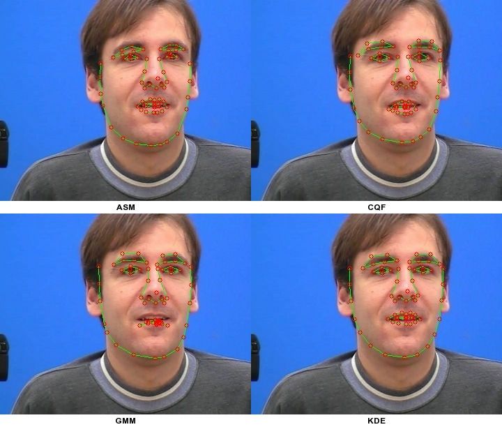
optimization proceeds by maximizing:
n
#
p({li = aligned}ni=1 | p) = p(li = aligned | xi ) (4)
i=1
with respect to the PDM parameters p, where xi is param-
eterized as in Equation (1) and dependence on the image I
is dropped for succinctness. It should be noted that some
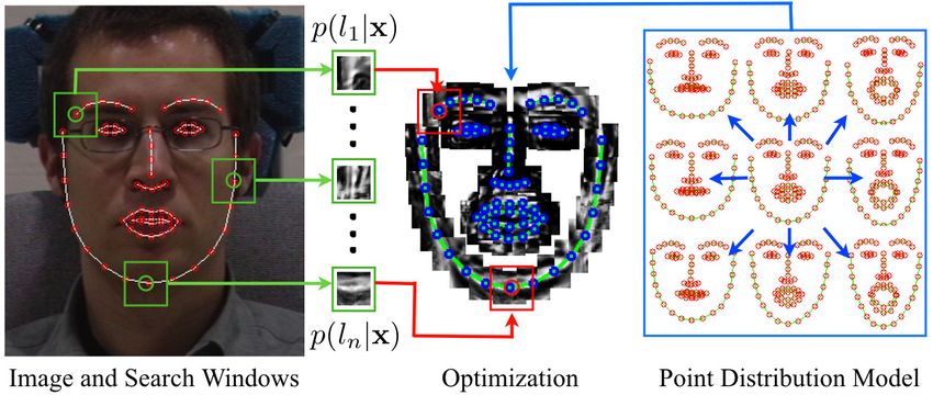
Figure 1. Illustration of CLM fitting and its two components: (i) forms of CLMs pose Equation (4) as minimizing the sum-
an exhaustive local search for feature locations to get the response mation of local energy responses (see §2.2).
maps {p(li = aligned|I, x)}n i=1 , and (ii) an optimization strategy The main difficulty in this optimization is how to avoid
to maximize the responses of the PDM constrained landmarks. local optima whilst affording an efficient evaluation. Treat-
ing Equation (4) as a generic optimization problem, one
may be tempted to utilize general purpose optimization
All instantiations of CLMs can be considered to be pur- strategies here. However, as the responses are typically
suing the same two goals: (i) perform an exhaustive local noisy, these optimization strategies have a tendency to
search for each PDM landmark around their current esti- be unstable. The simplex based method used in [4] has
mate using some kind of feature detector, and (ii) optimize been shown to perform reasonably for this task since it is
the PDM parameters such that the detection responses over a gradient-free based generic optimizer, which renders it
all of its landmarks are jointly maximized. Figure 1 illus- somewhat insensitive to measurement noise. However, con-
trates the components of CLM fitting. vergence may be slow when using this method, especially
for a complex PDM with a large number of parameters.
Exhaustive Local Search: In the first step of CLM fitting, a
likelihood map is generated for each landmark position by 2.2. Optimization Strategies
applying local detectors to constrained regions around the
current estimate. A number of feature detectors have been In this section, a review of current methods for CLM op-
proposed for this purpose. One of the simplest, proposed timization is presented. These methods entail replacing the
in [16], is the linear logistic regressor which gives the fol- true response maps, {p(li |x)}ni=1 , with simpler paramet-
lowing response map for the ith landmark2: ric forms and performing optimization over these instead
of the original response maps. As these parametric density
1 estimates are a kind of smoothed version of the original re-
p(li = aligned | I, x) = , (2) sponses, sensitivity to local minima is generally reduced.
1 + exp{α Ci (I; x) + β}
where li is a discrete random variable denoting whether the Active Shape Models: The simplest optimization strategy
ith landmark is correctly aligned or not, I is the image, x is for CLM fitting is that used in the Active Shape Model
a 2D location in the image, and Ci is a linear classifier: (ASM) [2]. The method entails first finding the location
within each response
! map for
" which the maximum was
Ci (I; x) = wiT I(y1 ) ; . . . ; I(ym ) + bi ,
! "
(3) attained: µ = µ1 ; . . . ; µn . The objective of the opti-
mization procedure is then to minimize the weighted least
with {yi }m squares difference between the PDM and the coordinates of
i=1 ∈ Ωx (i.e. an image patch). An advantage
of using this classifier is that the map can be computed us- the peak responses:
ing efficient convolution operations. Other feature detectors n
$
have also been used to great effect, such as the Gaussian Q(p) = wi "xi − µi "2 , (5)
likelihood [2] and the Haar-based boosted classifier [3]. i=1
Optimization: Once the response maps for each landmark where the weights {wi }ni=1 reflect the confidence over peak
have been found, by assuming conditional independence, response coordinates and are typically set to some func-
tion of the responses at {µi }ni=1 , making it more resistant
2 Not all CLM instances require a probabilistic output from the local towards such things as partial occlusion, where occluded
detectors. Some, for example [2, 5], only require a similarity measure or landmarks will be more weakly weighted.
a match score. However, these matching scores can be interpreted as the Equation (5) is iteratively minimized by taking a first or-
result of applying a monotonic function to the generating probability. For
example, the Mahalanobis distance used in [2] is the negative log of the der Taylor expansion of the PDM’s landmarks:
Gaussian likelihood. In the interest of clarity and succinctness, discussions
in this work assume that responses are probabilities. xi ≈ xci + Ji ∆p, (6)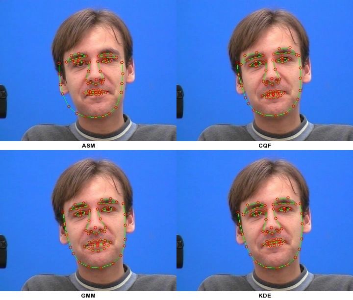
and solving for the parameter update:
             % n            &−1 n
               $                $
                       T
      ∆p =         wi Ji Ji        wi JTi (µi − xci ) ,       (7)
                 i=1                i=1

which is then applied additively to the current parameters:
p←p   ! + ∆p. Here,   " J = [J1 ; . . . ; Jn ] is the Jacobian and
xc = xc1 ; . . . ; xcn is the current shape estimate.                Figure 2. Response maps, p(li = aligned|x), and their approxi-
   From the probabilistic perspective introduced in §2.1, the        mations used in various methods, for the outer left eye corner, the
ASM’s optimization procedure is equivalent to approximat-            nose bridge and chin. Red crosses on the response maps denote the
ing the response maps with an isotropic Gaussian estimator:          true landmark locations. The GMM approximation has five cluster
                                                                     centers. The KDE approximations are shown for σ 2 ∈ {20, 5, 1}.
            p(li = aligned | x) ≈ N (x; µi , σi2 I),          (8)

where wi = σi−2 . With this approximation, taking the neg-           the solution of which is given by:
ative log of the likelihood in Equation (4) results in the ob-
                                                                                                   &−1
jective in Equation (5).
                                                                              % n                        n
                                                                               $                         $
                                                                      ∆p =             JTi Σ−1
                                                                                            i Ji                JTi Σ−1       c
                                                                                                                     i (µi − xi ) . (13)
Convex Quadratic Fitting: Although the approximation                             i=1                      i=1
described above is simple and efficient, in some cases it
may be a poor estimate of the true response map. Firstly, the
landmark detectors, such as the linear classifier described in       A Gaussian Mixture Model Estimate: Although the re-
§2.1, are usually imperfect in the sense that the maximum of         sponse map approximation in CQF may overcome some
the response may not always coincide with the correct land-          of the drawbacks of ASM, its process of estimation can be
mark location. Secondly, as the features used in detection           poor in some cases. In particular, when the response map is
consist of small image patches they often contain limited            strongly multimodal, such an approximation smoothes over
structure, leading to detection ambiguities. The simplest            the various modes (see the example response map for the
example of this is the aperture problem, where detection             eye corner in Figure 2).
confidence across the edge is better than along it (see exam-           To account for this, in [8] a Gaussian mixture model
ple response maps for the nose bridge and chin in Figure 2).         (GMM) was used to approximate the response maps:
   To account for these problems, a method coined con-                                              K
vex quadratic fitting (CQF) has been proposed recently [16].                                        $
                                                                         p(li = aligned | x) ≈            πik N (x; µik , Σik ),     (14)
The method fits a convex quadratic function to the negative
                                                                                                    k=1
log of the response map. This is equivalent to approximat-
ing the response map with a full covariance Gaussian:                where K denotes the number of modes and {πik }K      k=1 are
                                                                     the mixing coefficients for the GMM of the ith PDM land-
            p(li = aligned | x) ≈ N (x; µi , Σi ).            (9)
                                                                     mark. Treating the mode membership for each landmark,
The mean and covariance are maximum likelihood esti-                 {zi }ni=1 , as hidden variables, the maximum likelihood solu-
mates given the response map:                                        tion can be found using the expectation-maximization (EM)
        $                                    $                       algorithm, which maximizes:
Σi =         αix (x − µi ) (x − µi )T ; µi =   αix x,
                                                                                                   n $
                                                                                                     K
       x∈Ψxc                                       x∈Ψxc                                           #
             i                                           i
                                                       (10)                    p({li }ni=1 |p) =             pi (zi = k, li |xi ).   (15)
                                                                                                   i=1 k=1
where Ψxci is a 2D-rectangular grid centered at the current
landmark estimate xci (i.e. the search window), and:                   The E-step of the EM algorithm involves computing the
                      p(li = aligned | x)                            posterior distribution over the latent variables {zi }ni=1 :
            αix = '                           .              (11)
                    y∈Ψxc p(li = aligned | y)                                                  p(zi = k) p(li |zi = k, xi )
                              i
                                                                       p(zi = k | li , xi ) = 'K                                ,
With this approximation, the objective can be written as the                                   j=1 p(zi = j) p(li |zi = j, xi )
minimization of:                                                                                                               (16)
                       n
                                                                     where p(zi = k) = πik and:
                       $
          Q(∆p) =            "xci + Ji ∆p − µi "2Σ−1 ,       (12)
                       i=1
                                                   i                    p(li = aligned | zi = k, xi ) = N (xi ; µik , Σik ).         (17)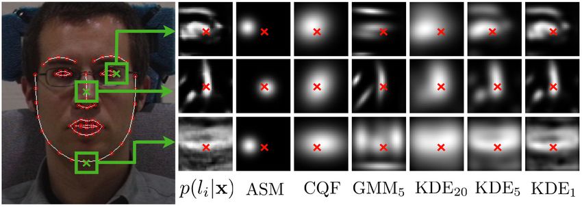
In the M-step, the expectation of the negative log of the        where αiµi is the normalized true detector response defined
complete data is minimized:                                      in Equation (11). With this representation the kernel centers
                 (      )n
                         #
                                                     *+          are fixed as defined through Ψxci (i.e. the grid nodes of the
  Q(p) = Eq(z) − log         p(li = aligned, zi |xi )   ,        search window). The mixing weights, αiµi , can be obtained
                            i=1                                  directly from the true response map. Since the response is
              ,n                                     (18)        an estimate of the probability that a particular location in the
where q(z) = i=1 pi (zi |li = aligned, xi ). Linearizing         image is the aligned landmark location, such a choice for the
the shape model as in Equation (6), this Q-function takes        mixing coefficients is reasonable. Compared to parametric
the form:                                                        representations, KDE has the advantage that no nonlinear
             n $
             $ K                                                 optimization is required to learn the parameters of its repre-
  Q(∆p) ∝              wik "Ji ∆p − yik "2Σ−1 + const, (19)      sentation. The only remaining free parameter is the variance
                                           ik
             i=1 k=1                                             of the Gaussian kernel, σ 2 , which regulates the smoothness
where wik = pi (zi = k|li = aligned, xi ) and yik = µik −        of the approximation. Since one of the main problems with
xci , the solution of which is given by:                         a GMM based representation is the computational complex-
         % n K                    &−1 n K                        ity and suboptimal nature of fitting a mixture model to the
           $$
                         T −1
                                       $$                        response maps, if σ 2 is set a-priori, then optimizing over
∆p =                wik Ji Σik Ji           wik JTi Σ−1
                                                     ik yik .    the KDE can be expected to be more stable and efficient.
         i=1 k=1                      i=1 k=1
                                                          (20)       Maximizing the objective in Equation (4) with a KDE
    Although the GMM is a better approximation of the re-        representations is nontrivial as the objective is nonlinear
sponse map compared to the Gaussian approximation in             and typically multimodal. However, in the case where no
CQF, it exhibits two major drawbacks. Firstly, the pro-          shape prior is placed on the way the PDM’s landmarks can
cess of estimating the GMM parameters from the response          vary, the problem reverts to independent maximizations of
maps is a nonlinear optimization in itself. It is only locally   the KDE for each landmark location separately. This is be-
convergent and requires the number of modes to be cho-           cause the landmark detections are assumed to be indepen-
sen a-priori. As GMM fitting is required for each PDM            dent, conditioned on the PDM’s parameterization. A com-
landmark, it constitutes a large computation overhead. Al-       mon approach for maximization over a KDE is to use the
though some approximations can be made, they are gener-          well known mean-shift algorithm [1]. It consists of fixed
ally suboptimal. For example, in [8], the modes are chosen       point iterations of the form:
as the K-largest responses in the map. The covariances are                                          -
                                                                                                       (τ )
                                                                                                                    .
                                                                                            αiµi N xi ; µi , σ 2 I
parametrized isotropically, with their variance heuristically        xi
                                                                       (τ +1)
                                                                              ←
                                                                                  $
                                                                                                          -             . µi ,
set as the scaled distance to the closest mode in the previous                                      i N x(τ ) ; y, σ 2 I
                                                                                         '
                                                                                µi ∈Ψxc    y∈Ψx  c
                                                                                                   αy        i
iteration of the CLM fitting algorithm. Such an approxima-                             i         i
                                                                                                                            (22)
tion allows an efficient estimate of the GMM parameters
                                                                 where τ denotes the time-step in the iterative process. This
without the need for a costly EM procedure at the cost of a
                                                                 fixed point iteration scheme finds a mode of the KDE, where
poorer approximation of the true response map.
                                                                 an improvement is guaranteed at each step by virtue of its
    The second drawback of the GMM response map ap-
                                                                 interpretation as a lower bound maximization [6]. Com-
proximation is that the approximated objective in Equa-
                                                                 pared to other optimization strategies, mean-shift is an at-
tion (15) is multimodal. As such, CLM fitting with the
                                                                 tractive choice as it does not use a step size parameter or a
GMM simplification is prone to terminating in local optima.
                                                                 line search. Equation (22) is simply applied iteratively until
Although good results were reported in [8], in that work the
                                                                 some convergence criterion is met.
PDM was parameterized using a mixture model as opposed
                                                                     To incorporate the shape model constraint into the opti-
to the more typical Gaussian parameterization, which places
                                                                 mization procedure, one might consider a two step strategy:
a stronger prior on the way the shape can vary.
                                                                 (i) compute the mean-shift update for each landmark, and
                                                                 (ii) constrain the mean-shifted landmarks to adhere to the
3. Subspace Constrained Mean-Shifts
                                                                 PDM’s parameterization using a least-squares fit:
   Rather than approximating the response maps for each                                    n /             /2
                                                                                                    (τ +1) /
                                                                                           $
PDM landmark using parametric models, we consider here                           Q(p) =      /xi − xi
                                                                                             /
                                                                                                           / .                (23)
the use of a nonparametric representation. In particular, we                               i=1
propose the use of a homoscedastic kernel density estimate
(KDE) with an isotropic Gaussian kernel:                         This is reminiscent of the ASM optimization strategy, where
                          $                                      the location of the response map’s peak is replaced with the
   p(li = aligned|x) ≈          αiµi N (x; µi , σ 2 I), (21)     mean-shifted estimate. Although such a strategy is attrac-
                          µi ∈Ψxc
                                  i
                                                                 tive in its simplicity, it is unclear how it relates to the global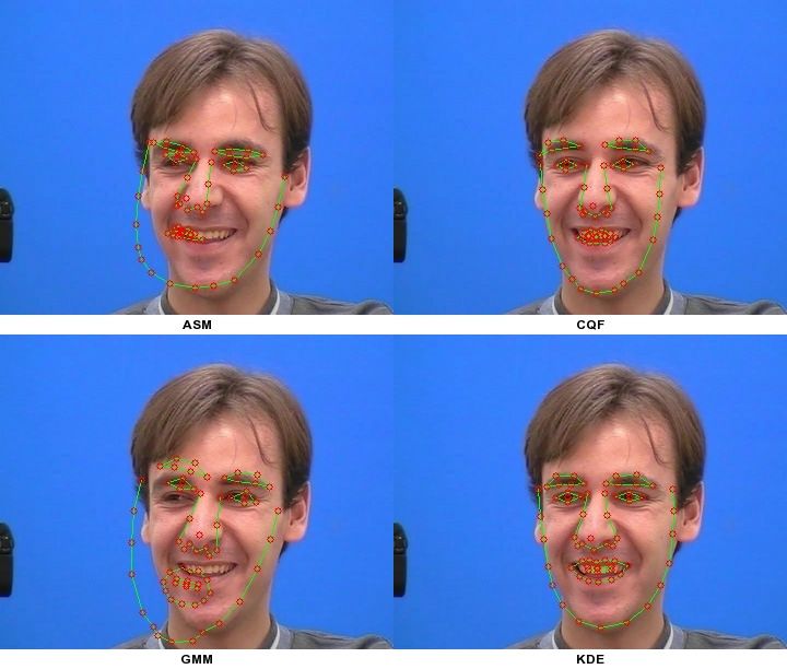
Algorithm 1 Subspace Constrained Mean-Shifts
Require: I and p.
 1: while not converged(p) do
 2:   Compute responses {Eqn. (2)}
 3:   Linearize shape model {Eqn. (6)}
 4:   Precompute pseudo-inverse of Jacobian (J† )
 5:   Initialize parameter updates: ∆p ← 0
 6:   while not converged(∆p) do
 7:      Compute mean-shifted landmarks {Eqn. (22)}
 8:      Apply subspace constraint {Eqn. (24)}                   Figure 3. Illustration of a the use of a precomputed grid for effi-
 9:   end while                                                  cient mean-shift. Kernel evaluations are precomputed between c
10:   Update parameters: p ← p + ∆p                              and all other nodes in the grid. To approximate the true kernel
11: end while                                                    evaluation, xi is assumed to coincide with c and the likelihood of
12: return p                                                     any response map grid location can be attained by a table lookup.

                                                                 tion is used to get within the convergence basin of the GMM
objective in Equation (4).
                                                                 approximation. However, such an approach is inelegant and
    Given the form of the KDE representation in Equa-
                                                                 affords no guarantee that the mode of the Gaussian approx-
tion (21), one can treat it simply as a GMM. As such, the
                                                                 imation lies within the convergence basin of the GMM’s.
discussions in §2.2 on GMMs are directly applicable here,
                                                                     With the KDE approximation in SCMS a more elegant
replacing the number of candidates K with the number of
                                                                 approach can be devised, whereby the complexity of the
grid nodes in the search window Ψxci , the mixture weights
                                                                 response map estimate is directly controlled by the variance
πik with αiµi , and the covariances Σik with the scaled iden-    of the Gaussian kernel (see Figure 2). The guiding principle
tity σ 2 I. When using the linearized shape model in Equa-       here is similar to that of optimizing on a Gaussian pyramid.
tion (6) and maximizing the global objective in Equation (4)     It can be shown that when using Gaussian kernels, there
using the EM algorithm, the solution for the so called Q-        exists a σ 2 < ∞ such that the KDE is unimodal, regardless
function of the M-step takes the form:                           of the distribution of samples [13]. As σ 2 is reduced, modes
                0
                  (τ +1)
                                                      1          divide and smoothness of the objective’s terrain decreases.
     ∆p = J† x1          − xc1 ; . . . ; x(τ
                                          n
                                             +1)
                                                 − xcn , (24)    However, it is likely that the optimum of the objective at
                                                                 a larger σ 2 is closest to the desired mode of the objective
                                                     (τ +1)
where J† denotes the pseudo-inverse of J, and xi          is     with a smaller σ 2 , promoting its convergence to the correct
the mean shifted update for the ith landmark given in Equa-      mode. As such, the policy under which σ 2 is reduced acts to
tion (22). This is simply the Gauss Newton update for the        guide optimization towards the global optimum of the true
least squares PDM constraint in Equation (23). As such, un-      objective.
der a linearized shape model, the two step strategy for max-         Drawing parallels with existing methods, as σ 2 → ∞
imizing the objective in Equation (4) with a KDE represen-       the SCMS update approaches the solution of a homoscedas-
tation shares the properties of a general EM optimization,       tic Gaussian approximated objective function. As σ 2 is re-
namely: provably improving and convergent. The complete          duced, the KDE approximation resembles a GMM approx-
fitting procedure, which we will refer to as subspace con-       imation, where the approximation for smaller σ 2 settings is
strained mean-shifts (SCMS), is outlined in Algorithm 1. In      similar to a GMM approximation with more modes.
the following, two further innovations are proposed, which
address difficulties regarding local optima and the compu-       Precomputed Grid: In the KDE representation of the re-
tational expense of kernel evaluations.                          sponse maps, the kernel centers are placed at the grid nodes
                                                                 defined by the search window. From the perspective of
Kernel Width Relaxation: The response map approxi-               GMM fitting, these kernels represent candidates for the true
mations discussed in §2.2 can be though of as a form of          landmark locations. Although no optimization is required
smoothing. This explains the relative performance of the         for determining the number of modes, their centers and
various methods. The Gaussian approximations smooth the          mixing coefficients, the number of candidates used here is
most but approximate the true response map the poorest,          much larger than what would typically be used in a general
whereas smoothing effected by the GMM is not as aggres-          GMM estimate (i.e. GMM based representations typically
sive but exhibits of a degree of sensitivity towards local op-   use K < 10, whereas the search window size typically has
tima. One might consider using the Gaussian and GMM              > 100 nodes). As such, the computation of the posterior
approximations in tandem, where the Gaussian approxima-          in Equation (16) will be more costly. However, if the vari-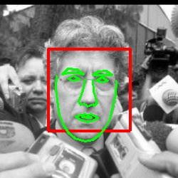
MultiPieFittingCurve                                                            XM2VTSFittingCurve
                       1                                                                               1
                                 ASM(88ms)                                                                        ASM(84ms)
                                 CQF(98ms)                                                                        CQF(93ms)
                     0.8                                                                              0.8
ProportionofImages

                                                                                 ProportionofImages
                               GMM(2410ms)                                                                      GMM(2313ms)
                                KDE(121ms)                                                                       KDE(117ms)
                     0.6                                                                              0.6

                     0.4                                                                              0.4

                     0.2                                                                              0.2

                       0                                                                               0
                           0       2        4         6        8        10                                  0      2        4      6        8   10
                                         ShapeRMSError                                                                   ShapeRMSError
                                            (a)                                                                            (b)
                     Figure 4. Fitting Curves for the ASM, CQF, GMM and KDE optimization strategies on the MultiPie and XM2VTS databases.

ance σ 2 is known a-priori, then some approximations can                           2360 frontal face images of 295 subjects for which ground
be made to significantly reduce computational complexity.                          truth annotations are publicly available but different from
   The main overhead when computing the mean-shift up-                             the 68-point markup we have for MultiPie. XM2VTS con-
date is in evaluating the Gaussian kernel between the current                      tains neutral expression only whereas MultiPie contains sig-
landmark estimate and every grid node in the response map.                         nificant expression variations. A 4-fold cross validation
Since the grid locations are fixed and σ 2 is assumed to be                        was performed on both MultiPie and XM2VTS, separately,
known, one might choose to precompute the kernel for var-                          where the images were partitioned into three sets of non-
ious settings of xi . In particular, a simple choice would be                      overlapping subject identities. In each trial, three partitions
to precompute these values along a grid sampled at or above                        were used for training and the remainder for testing.
the resolution of the response map grid Ψxci . During fitting                          On these databases we compared four types of optimiza-
one simply finds the location in this grid closest to the cur-                     tion strategies: (i) ASM [2], (ii) CQF [16], (iii) GMM [8],
rent estimate of a PDM landmark and estimate the kernel                            and (iv) the KDE method proposed in §3. For GMM, we
evaluations by assuming the landmark is actually placed at                         empirically set K = 5 and used the EM algorithm to es-
that node (see Figure 3). This only involves a table lookup                        timate the parameters of the mixture model. For KDE, we
and can be performed efficiently. The higher the granularity                       used a variance relaxation policy of σ 2 = {20, 10, 5, 1} and
of the grid the better the approximation will be, at the cost                      a grid spacing of 0.1-pixels in its efficient approximation. In
of greater storage requirements but without a significant in-                      all cases the linear logistic regressor described in §2.1 was
crease in computational complexity.                                                used. The local experts were (11 × 11)-pixels in size and
   Although such an approximation ruins the strictly im-                           the exhaustive local search was performed over a (15 × 15)-
proving properties of EM, we empirically show in §4 that                           pixel window. As such, the only difference between the var-
accurate fitting can still be achieved with this approxima-                        ious methods compared here is their optimization strategy.
tion. In our implementation, we found that such an approx-                         In all cases, the scale and location of the model was initial-
imation reduced the average fitting time by one half.                              ized by an off-the-shelf face detector, the rotation and non-
                                                                                   rigid parameters in Equation (1) set to zero (i.e. the mean
4. Experiments                                                                     shape), and the model fit until the optimization converged.
                                                                                       Results of these experiments can be found in Figure 4,
                                                                                   where the graphs (fitting curves) show the proportion of im-
Database Specific Experiments: We compared the various                             ages at which various levels of maximum perturbation was
CLM optimizations strategies discussed above on the prob-                          exhibited, measured as the root-mean-squared (RMS) er-
lem of generic frontal face fitting on two databases: (i) the                      ror between the ground truth landmarks and the resulting
CMU Pose, Illumination and Expression Database (Multi-                             fit. The average fitting times for the various methods on a
Pie) [7], and (ii) the XM2VTS database [12]. The Mul-                              2.5GHz Intel Core 2 Duo processor are shown in the legend.
tiPie database is annotated with a 68-point markup used                                The results show a consistent trend in the relative per-
as ground truth landmarks. We used 762 frontal face im-                            formance of the four methods. Firstly, CQF has the capac-
ages of 339 subjects. The XM2VTS database consists of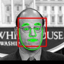
20
                                 ASM
                                 GMM
                        15        CQF
        ShapeRMSError

                                  KDE

                        10

                        5

                        0
                             0          1000             2000                 3000                 4000                 5000
                                                                  Frame
Figure 5. Top row: Tracking results on the FGNet Talking Face database for frames {0, 1230, 4200}. Clockwise from top left are fitting
results for ASM, CQF, KDE and GMM. Bottom: Plot of shape RMS error from ground truth annotations throughout the sequence.

ity to significantly outperform ASM. As discussed in §2.2             conducted as it requires the tedious process of annotating
this is due to CQF’s ability to account for directional un-           new images with the PDM configuration of the training set.
certainty in the response maps as well as being more ro-              Here, we utilize the freely available FGNet talking face se-
bust towards outlying responses. However, CQF has a ten-              quence3. Quantitative analysis on this sequence is possible
dency to over-smooth the response maps, leading to limited            since ground truth annotations are available in the same for-
convergence accuracy. GMM shows an improvement in ac-                 mat as that in XM2VTS. We initialize the model using a
curacy over CQF as shown by the larger number of sam-                 face detector in the first frame and fit consecutive frames us-
ples that converged to smaller shape RMS errors. However,             ing the PDM’s configuration in the previous frame as an ini-
it has the tendency to terminate in local optima due to its           tial estimate. The same model used in the database-specific
multimodal objective. This can be seen by its poorer per-             experiments was used here, except that it was trained on
formance than CQF for reconstructions errors above 4.2-               all images in XM2VTS. In Figure 5, the shape RMS error
pixels RMS in MultiPie and 5-pixels RMS in XM2VTS.                    for each frame is plotted for the four optimization strate-
In contrast, KDE is capable of attaining even better accu-            gies being compared. The relative performance of the var-
racies than GMM but still retains a degree of robustness              ious strategies is similar to that in the database-specific ex-
towards local optima, where its performance over grossly              periments, with KDE yielding the best performance. ASM
misplaced initializations is comparable to CQF. Finally, de-          and GMM are particularly unstable on this sequence, with
spite the significant improvement in performance, KDE ex-             GMM loosing track at around frame 4200, and fails to re-
hibits only a modest increase in computational complexity             cover until the end of the sequence.
compared to ASM and CQF. This is in contrast to GMM                       Finally, we performed a qualitative analysis of KDE’s
that requires much longer fitting times, mainly due to the            performance on the Faces in the Wild database [9]. It con-
complexity of fitting a mixture model to the response maps.           tains images taken under varying lighting, resolution, im-
                                                                      age noise and partial occlusion. As before, the model was
Out-of-Database Experiments: Testing the performance                  initialized using a face detector and fit using the XM2VTS
of fitting algorithms on images outside of a particular
database is more meaningful as it gives a better indication             3 http://www-prima.inrialpes.fr/FGnet/data/
on how well the method generalizes. However, this is rarely           01-TalkingFace/talking_face.html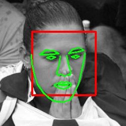
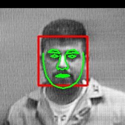
Figure 6. Example fitting results on the Faces in the Wild database using a model trained using the XM2VTS database. Top row: Male
subjects. Middle row: female subjects. Bottom row: partially occluded faces.

trained model. Some fitting results are shown in Figure 6.          [5] D. Cristinacce and T. F. Cootes. Feature Detection and
Results suggest that KDE exhibits a degree of robustness                Tracking with Constrained Local Models. In EMCV, pages
towards variations typically encountered in real images.                929–938, 2004.
                                                                    [6] M. Fashing and C. Tomasi. Mean Shift as a Bound Opti-
                                                                        mization. PAMI, 27(3), 2005.
5. Conclusion                                                       [7] R. Gross, I. Matthews, S. Baker, and T. Kanade. The
   The optimization strategy for deformable model fitting               CMU Multiple Pose, Illumination and Expression (Mul-
                                                                        tiPIE) Database.     Technical report, Robotics Institute,
was investigated in this work. Various existing methods
                                                                        Carnegie Mellon University, 2007.
were posed within a consistent probabilistic framework
                                                                    [8] L. Gu and T. Kanade. A Generative Shape Regularization
where they were shown to make different parametric ap-
                                                                        Model for Robust Face Alignment. In ECCV’08, 2008.
proximations to the true likelihood maps of landmark loca-
                                                                    [9] G. B. Huang, M. Ramesh, T. Berg, and E. Learned-Miller.
tions. A new approximation was then proposed that uses                  Labeled Faces in the Wild: A Database for Studying Face
a nonparametric representation. Two further innovations                 Recognition in Unconstrained Environments. Technical Re-
were proposed in order to reduce computational complexity               port 07-49, University of Massachusetts, Amherst, 2007.
and avoid local optima. The proposed method was shown to           [10] X. Liu. Generic Face Alignment using Boosted Appearance
outperform three other optimization strategies on the task of           Model. In CVPR, pages 1–8, 2007.
generic face fitting. Future work will involve investigations      [11] I. Matthews and S. Baker. Active Appearance Models Revis-
into the effects of different local detectors types and shape           ited. IJCV, 60:135–164, 2004.
priors on the optimization strategies.                             [12] K. Messer, J. Matas, J. Kittler, J. Lüttin, and G. Maitre.
                                                                        XM2VTSDB: The Extended M2VTS Database. In AVBPA,
                                                                        pages 72–77, 1999.
References                                                         [13] M. A. C.-P. nán and C. K. I. Williams. On the Number of
 [1] Y. Cheng. Mean Shift, Mode Seeking, and Clustering. PAMI,          Modes of a Gaussian Mixture. Lecture Notes in Computer
     17(8):790–799, 1995.                                               Science, 2695:625–640, 2003.
 [2] T. F. Cootes and C. J. Taylor. Active Shape Models - ‘Smart   [14] M. H. Nguyen and F. De la Torre Frade. Local Minima Free
     Snakes’. In BMVC, pages 266–275, 1992.                             Parameterized Appearance Models. In CVPR, 2008.
 [3] D. Cristinacce and T. Cootes. Boosted Active Shape Models.    [15] J. Saragih and R. Goecke. A Nonlinear Discriminative Ap-
     In BMVC, volume 2, pages 880–889, 2007.                            proach to AAM Fitting. In ICCV, 2007.
                                                                   [16] Y. Wang, S. Lucey, and J. Cohn. Enforcing Convexity for Im-
 [4] D. Cristinacce and T. F. Cootes. A Comparison of Shape
                                                                        proved Alignment with Constrained Local Models. In CVPR,
     Constrained Facial Feature Detectors. In FG, pages 375–
                                                                        2008.
     380, 2004.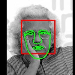
You can also read