Simplified Analysis of Measurement Data from A Rapid E. coli qPCR Method (EPA Draft Method C) Using A Standardized Excel Workbook - MDPI
←
→
Page content transcription
If your browser does not render page correctly, please read the page content below
water
Article
Simplified Analysis of Measurement Data from A
Rapid E. coli qPCR Method (EPA Draft Method C)
Using A Standardized Excel Workbook
Molly J. Lane 1 , James N. McNair 1 , Richard R. Rediske 1, *, Shannon Briggs 2 ,
Mano Sivaganesan 3 and Richard Haugland 3
 1   Annis Water Resources Institute, Grand Valley State University, Muskegon, MI 49401, USA;
     lanemoll@gvsu.edu (M.J.L.); mcnairja@gvsu.edu (J.N.M.)
 2   Michigan Department of Environment, Great Lakes, and Energy (EGLE), 525 W. Allegan St., Lansing,
     MI 48909, USA; BRIGGSS4@michigan.gov
 3   Center for Environmental Measurement and Modeling, Office of Research and Development, U.S. EPA,
     Cincinnati, OH 45268, USA; Sivaganesan.Mano@epa.gov (M.S.); haugland.rich@epa.gov (R.H.)
 *   Correspondence: redisker@gvsu.edu

 Received: 14 February 2020; Accepted: 6 March 2020; Published: 11 March 2020

 Abstract: Draft method C is a standardized method for quantifying E. coli densities in recreational
 waters using quantitative polymerase chain reaction (qPCR). The method includes a Microsoft
 Excel workbook that automatically screens for poor-quality data using a set of previously proposed
 acceptance criteria, generates weighted linear regression (WLR) composite standard curves, and
 calculates E. coli target gene copies in test samples. We compared standard curve parameter values
 and test sample results calculated with the WLR model to those from a Bayesian master standard
 curve (MSC) model using data from a previous multi-lab study. The two models’ mean intercept
 and slope estimates from twenty labs’ standard curves were within each other’s 95% credible or
 confidence intervals for all labs. E. coli gene copy estimates of six water samples analyzed by eight
 labs were highly overlapping among labs when quantified with the WLR and MSC models. Finally,
 we compared multiple labs’ 2016–2018 composite curves, comprised of data from individual curves
 where acceptance criteria were not used, to their corresponding composite curves with passing
 acceptance criteria. Composite curves developed from passing individual curves had intercept and
 slope 95% confidence intervals that were often narrower than without screening and an analysis
 of covariance test was passed more often. The Excel workbook WLR calculation and acceptance
 criteria will help laboratories implement draft method C for recreational water analysis in an efficient,
 cost-effective, and reliable manner.

 Keywords: E. coli; recreational water quality; methods development; qPCR; standard curve model

1. Introduction
      Quantitative real-time polymerase chain reaction (qPCR) has become a valuable tool for scientific
research due to its specificity, sensitivity, and analysis speed. The technique has been widely
implemented in environmental science and public health fields, where it is currently under regulatory
consideration as a means for the rapid testing of fecal indicator bacteria in recreational water samples.
Because contact with fecal contaminated water increases the likelihood of developing gastrointestinal
(GI) illnesses [1,2], public beaches are routinely monitored for the presence of Enterococcus or Escherichia
coli (E. coli) to alert beach managers and recreators to incidences of fecal contamination, thereby
reducing the risk of recreational exposure [3,4]. Furthermore, current United States Environmental
Protection Agency (U.S. EPA) guidelines for microbial recreational water quality are based on the

Water 2020, 12, 775; doi:10.3390/w12030775                                       www.mdpi.com/journal/water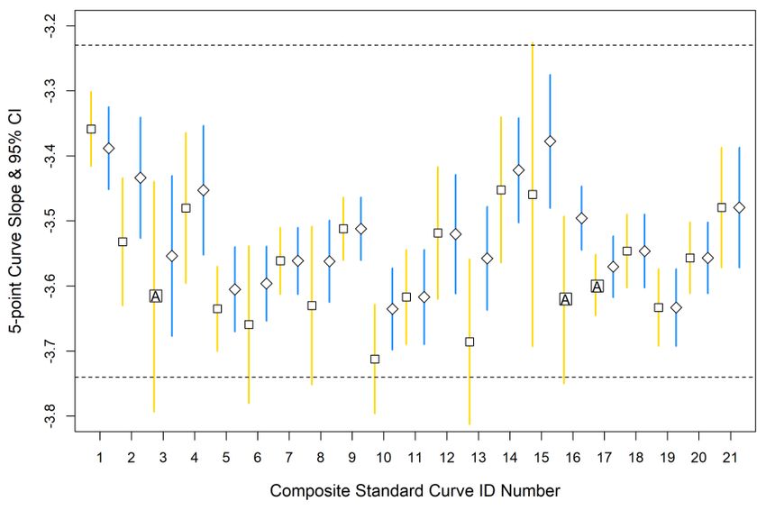
Water 2020, 12, 775                                                                                 2 of 15

risks of contracting GI illness associated with different levels of these organisms or a specific sequence
fragment of their deoxyribonucleic acid (DNA) [4].
      At present, there are no epidemiological studies directly demonstrating a relationship between
E. coli measurements from a qPCR method and swimming related illnesses. Previous studies have
demonstrated, however, that results from an E. coli qPCR method and an approved E. coli culture
method, where a health relationship has been established, can show a high degree of correlation and
lead to similar recreational beach management decisions [5]. Additional studies have been conducted
in 2016–2018 in the state of Michigan to similarly assess the relationships between E. coli culture
methods and an E. coli qPCR method (draft method C) developed by the U.S. EPA (S. Briggs and
R. Haugland, personal communications). Any water quality testing method that is intended to be
applied across many localities must be robust to the varying environmental conditions intrinsic to
water bodies (i.e., turbidity and organic content), easily performed by laboratory analysts, and shown
to produce reliable, consistent, and accurate results. Draft method C is being developed by the U.S.
EPA as a standardized qPCR method for the quantification of E. coli that would provide same-day
microbial water quality results. Quantification by qPCR is achieved by fitting a standard curve, also
called a calibration curve, to data consisting of the base-10 logarithms (log10 ) of a series of known
quantities of target DNA sequences (the standards) and their corresponding measured threshold cycles
(Ct values) [6,7]. The fitted standard curve is then used to estimate target gene copy quantities in
recreational water samples based on Ct measurements from DNA extracts of these samples.
      Early versions of draft method C used a hierarchical Bayesian standard curve model to generate a
master standard curve (MSC) [8]. While useful for accurately accounting for the uncertainty in E. coli
estimates, such determinations of uncertainty are currently not required for routine beach monitoring
and the Bayesian MSC model requires specialized statistical software and expertise that could make
it impractical for use by labs with limited statistical capabilities. Consequently, a more user-friendly
standard curve model was pursued.
      The current version of draft method C, being implemented in a Microsoft Excel workbook
provided in the supplemental material, uses a classical weighted linear regression (WLR) standard
curve model. The draft method C Excel workbook is designed to generate a composite standard curve
from the pooled Ct measurement data from a minimum of four independent individual standard
curves. The Excel workbook then uses the composite standard curve to automatically quantify mean E.
coli target gene copies in test sample DNA extracts, e.g., recreational water samples. Another feature
of the current version of draft method C that was not used in the previous Bayesian MSC model is a
set of quality control acceptance criteria proposed by Sivaganesan et al., [9]. The workbook requires
criteria to be met for the y-intercept (hereafter referred to as intercept) and slope of both individual
and composite standard curves, as well as for positive and negative controls that are included when
analyzing both standard curve and test sample plates. The Excel workbook also uses an analysis of
covariance (ANCOVA) model to evaluate intercept and slope values of individual standard curves
that meet the acceptance criteria to determine if any large deviations are present. The use of quality
assurance and quality control procedures, including the standard curve acceptance criteria, should
help to ensure that data quality is maintained [9,10].
      To increase U.S. EPA and end user confidence in the current version of draft method C, it was
considered important to demonstrate the comparability of the WLR model used in the Excel workbook
to the previously used Bayesian MSC model. Consequently, the first goal of this study was to determine
whether the WLR model yielded results that were comparable to those of the MSC model. This question
was first addressed by determining the similarity of mean composite standard curve intercept and
slope estimates obtained from the WLR and MSC models using the Ct values from the DNA standards
from a large multi-lab study conducted in 2016 [9]. Furthermore, the variability of draft method C
results was previously defined from quantified test sample estimates obtained using the Bayesian
MSC model in a separate 2016 study [11]. Thus, we further addressed the question by determining the
similarity of E. coli target gene copy estimates using MSC standard curves from the 2016 multi-lab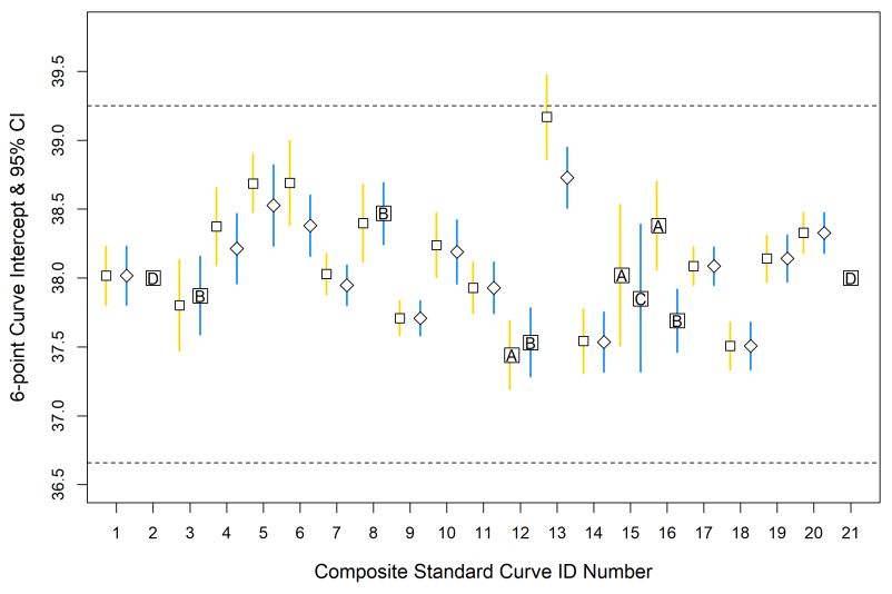
Water 2020, 12, 775                                                                               3 of 15

study [9] and WLR composite curves generated by the same labs in subsequent studies, together with
the same test sample measurement data from 2016 [11] for both. A second goal of this study was to
evaluate the impact of implementing the intercept and slope acceptance criteria on the variability and
reliability of WLR composite curves generated by multiple labs using the Excel workbook during
ongoing recreational water sample analyses in 2016–2018 with draft method C. These evaluations were
performed by comparing the variability of WLR standard curve intercept and slope estimates and
the ability of the contributing individual curves to pass the ANCOVA test before and after screening
individual standard curve data with the proposed acceptance criteria. The frequencies at which
the individual standard curves passed or failed also were used as a gauge of lab performance and
for troubleshooting logistical and technical problems with standards analyses during the ongoing
2016–2018 studies.

2. Materials and Methods

2.1. Participants
     The present study includes three assessments, each of which employed data from labs that
volunteered to participate. Comparison of the WLR and MSC models used data from the 2016 study [9],
which included a diverse group of twenty-one labs from across the midwestern and southeastern
United States (Table 1). Data for comparing test sample estimates and the impact of acceptance criteria
came from a subset of labs in the State of Michigan, which is the only state that has moved forward thus
far with draft method C in practice. Moreover, the decision to include labs for the test sample analysis
comparisons was based on the completeness of their accepted data sets from the 2016 study [11] and
whether ongoing WLR composite curves were available from these labs. Data from eight labs were
used for the test sample analysis comparisons and data from eleven labs were used for determining
the impact of acceptance criteria analysis. Government, university and county health department labs
were represented in all three assessments. Each lab was assigned a unique numeric code (1–21) to
maintain anonymity when presenting results.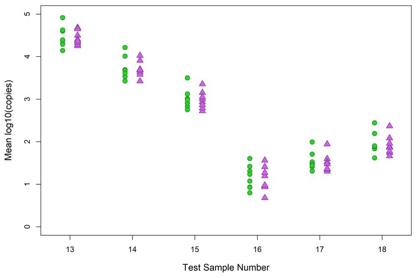
Water 2020, 12, 775                                                                                                                                                             4 of 15

      Table 1. Participating labs. List of labs participating in the three assessments conducted in the present study. An ‘x’ indicates that data from the respective lab (row)
      were used in the respective assessment (column). (WLR = Weighted Linear Regression; MSC = Master Standard Curve).

                                                                                                                                                   Acceptance Criteria Impact
                               Laboratory                                       Location               WLR vs. MSC       Test Sample Analysis
                                                                                                                                                          (2016–2018)
         Central Michigan District Health Dept., Assurance Water
                                                                        Gladwin, MI 48624, USA              x                                                  x
                                 Laboratory
                     City of Racine Public Health Dept.                   Racine, WI 53403, USA             x
            Ferris State University, Shimadzu Core Laboratory           Big Rapids, MI 49307, USA           x                     x                            x
          Georgia Southern University, Dept. of Environmental
                                                                       Statesboro, GA 30458, USA            x
                              Health Sciences
          Grand Valley State University, Annis Water Resources
                                                                        Muskegon, MI 49441, USA             x                     x                            x
                                  Institute
        Health Dept. of Northwest Michigan, Northern Michigan
                                                                         Gaylord, MI 49735, USA             x
                            Regional Laboratory
           Kalamazoo County Health and Community Services
                                                                       Kalamazoo, MI 49001, USA             x                     x                            x
                                 Laboratory
         Lake Superior State University, Environmental Analysis
                                                                      Sault St. Marie, MI 49783, USA        x                     x                            x
                                 Laboratory
                    Marquette Area Wastewater Facility                  Marquette, MI 49855, USA            x                                                  x
         Michigan State University, Department of Fisheries and
                                                                       East Lansing, MI 48824, USA          x
                                  Wildlife
        Northeast Ohio Regional Sewer District, Environmental and     Cuyahoga Heights, OH 44125,
                                                                                                            x
                        Maintenance Services Center                                USA
              Oakland County Health Division Laboratory                 Pontiac, MI 48341, USA              x                     x                            x
                 Oakland University, HEART Laboratory                  Rochester, MI 48309, USA             x                     x                            x
            U.S. EPA National Exposure Research Laboratory             Cincinnati, OH 45268, USA            x                     x                            x
         United States Geological Survey, Upper Midwest Water
                                                                         Lansing, MI 48911, USA             x                                                  x
                               Science Center
         U.S. National Parks Service, Sleeping Bear Dunes Water
                                                                         Empire, MI 49360, USA              x
                                 Laboratory
                Saginaw County Health Dept. Laboratory                  Saginaw, MI 48302, USA              x
                                                                       University Center, MI 48710,
            Saginaw Valley State University, Dept. of Chemistry                                             x                     x                            x
                                                                                  USA
         University of Illinois at Chicago, School of Public Health     Chicago, IL 60612, USA              x
         University of North Carolina at Chapel Hill, Institute of
                                                                      Morehead City, NC 28557, USA          x
                               Marine Sciences
        University of Wisconsin-Oshkosh, Environmental Research
                                                                        Oshkosh, WI 54901, USA              x
                                 Laboratory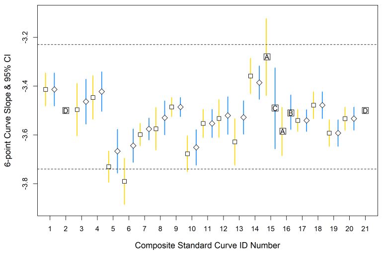
Water 2020, 12, 775                                                                                   5 of 15

2.2. qPCR Analyses
     The qPCR assays (EC23S857 E. coli [12] and the Sketa22 (salmon DNA sample processing control)),
methods of DNA extractions, and qPCR analysis methods used for all parts of this study are described
by Sivaganesan et al., [9] and Aw et al., [11]. Methods used to construct the Bayesian MSCs are described
in detail by Sivaganesan et al., [9] and methods used to construct the WLR standard curves are described
below. The standards used to generate the WLR and Bayesian MSC standard curve models were
prepared and quantified at the U.S. EPA Cincinnati laboratory, as described by Sivaganesan et al., [13].
Participating labs received five standards (where standard number 5 was the lowest concentration)
that were shipped overnight on dry ice from a central lab. A sixth standard was prepared on site by
most of the labs by 1:1 (v:v) dilution of standard 5 with AE buffer. Each year, all labs used a single lot of
TaqMan™ Environmental MM 2.0 (Thermo Fisher Scientific, Waltham, MA, USA) that was confirmed
to have little or no underlying E. coli DNA contamination for standard curve and test sample analysis.

2.3. Standard Curves in the Draft Method C Excel Workbook
     Upon completion of instrument analysis of the standards, data were exported and the resulting
Ct values copied into the draft method C Excel workbook where the WLR model was fitted. The WLR
model has the form
                                     Yijk = αi + βi log10 (Xj ) + εijk                          (1)

where Yijk is the observed Ct value for replicate k of standard concentration j in run i; αi and βi are the
intercept and slope, respectively, for run i; Xj is the known copy number (standard concentration) in
standard j, and εijk is the statistical error in the observed threshold cycle. Because variation among
observed Ct values in replicates of each standard is approximately inversely proportional to the
logarithm of the copy number, the model was fitted to data for each run i by weighted least-squares
linear regression to stabilize the variance, with multiplicative weight wj = log10 (Xj ) applied to squared
errors for each standard j. A separate WLR was fitted to Ct values from each individual standard
curve, and the externally Studentized residuals [14] (p. 20) were examined to identify and remove
up to two outliers from the triplicate analyses of standards from each individual standard curve’s
data set if needed. The WLR model was then re-fitted to the retained data for each analysis, and the
intercept and slope values for each individual standard curve were assessed for acceptability based
on the proposed standard curve acceptance criteria developed for draft method C (36.66 to 39.25 for
intercept, −3.23 to −3.74 for slope) [9]. The Excel workbook also screens for other quality control
parameters such as the positive control (calibrator) Sketa22 (18.58 to 22.01) and E. Coli assay (26.48
to 29.63) Ct values; and negative controls such as no-template control (NTC), un-spiked filter (filter
blank), and lower limit of quantification (LLOQ) Ct values, which are determined directly from each
composite standard curve and not the global value proposed in Sivaganesan et al., [9]. The LLOQ was
the Ct value of the estimated 95% confidence interval (CI) upper bound at the lowest concentration.
If an individual standard curve met these criteria it was considered ‘passing’; if a curve failed one or
more of the criteria, it was considered ‘failing’. The intercept and slope data for each passing standard
curve from each lab were then assessed by the workbook with an ANCOVA model to determine if
there was strong evidence (α = 0.01) that any parameter estimates differed among runs. If there was
no strong evidence of a difference (p > 0.01 for both parameters), results from the individual curves
were pooled, and a WLR model was fitted to estimate the composite curve intercept, slope, and 95%
CIs for each lab. The current version of the draft method C workbook requires a minimum of four
passing individual curves to generate the composite curve used to analyze recreational water samples.
However, for the purposes of our study, in six instances, four of which were from the 6-point standard
curves (Supplementary Table S1), the minimum of four individual standard curves was relaxed to
three to include data from all actively participating Michigan network labs.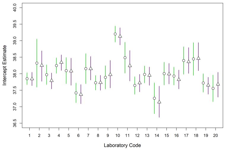
Water 2020, 12, 775                                                                                   6 of 15

2.4. Data Analysis

2.4.1. WLR and Bayesian MSC Standard Curve Model Comparisons
     In 2016, twenty-one labs (Table 1, column 3) analyzed four or five individual standard curves for
a total of ninety-one curves analyzed. Mean intercept and slope estimates from the Bayesian MSC
model for individual labs were taken from Sivaganesan et al., [9]; the 95% Bayesian Credible Intervals
(BCIs) are provided in the supplemental material (Supplementary Table S2). WLR composite curve
intercept and slope estimates were determined as described in Section 2.3. The ANCOVA evaluation
and standard curve acceptance criteria were applied to the WLR model only (not the Bayesian MSC
model) using the Excel workbook. Mean intercept and slope estimates, and corresponding 95% BCIs
and CIs, from the Bayesian MSC and WLR models, respectively, were plotted using R software (V 3.6.1,
Vienna, Austria) for a visual comparison of each lab’s results.

2.4.2. Comparison of Test Sample E. coli Estimates by the Two Models
     Data from eight labs were used for this assessment. Ct measurement data from one filter each,
analyzed in duplicate, of a six-sample (Table 2) subset of the eighteen water samples described in
Aw et al., [11] and corresponding positive control (calibrator) Ct data from three filters (analyzed in
duplicate producing six measurements) from the 2016 study were chosen for further analysis in our
study. In each case, data from only the first of three replicate test sample filters in the 2016 study were
selected in accordance with the common practice of analyzing only one filter per water sample for
beach monitoring in Michigan. The test sample data represented nearly the entire range of E. coli
concentrations examined in the 2016 study. Furthermore, test sample data were from labs that met all
draft method C quality control criteria for these samples and had ongoing 2016–2018 WLR composite
curves available for comparison. E. coli log10 target gene copy estimates were determined using the
mean standard curve intercept and slope values from the 2016 Bayesian MSC model and mean values
from one corresponding ongoing WLR composite curve (nearest in time to the 2016 study) from each
lab. E. coli target gene copy estimates were determined, as per the draft method C Excel workbook,
from the intercept and slope values and from the mean positive control (calibrator) and test sample Ct
values using the following formula:

                                Usmp = (Ysmp − (Ssmp − Scal ) − αstd )/βstd                              (2)

where Usmp is the estimated mean sample log10 copy number of the target gene, Ysmp is the mean
sample E. coli Ct, Ssmp is the mean sample Sketa22 Ct, Scal is the mean calibrator Sketa22 Ct, αstd is
the estimated intercept for the standard curve, and βstd is the estimated slope of the standard curve.
This formula adjusts the sample E. coli Ct value (Ysmp ) to remove any anomalous changes due to
interference or facilitation by the test sample matrix, as indicated by the difference between the sample
and positive control (calibrator) Sketa22 Ct values (|Ssmp − Scal | > 0), then uses this adjusted Ct value in
the inverted WLR regression equation to determine the corresponding log10 copy number of the target
gene in the sample (Usmp ). Mean E. coli target gene copy concentrations from the two models were
then plotted side-by-side using R Software (V3.6.1) and visually compared. Individual standard curve
acceptance criteria and the ANCOVA evaluation were assessed in the draft method C Excel workbook
for the WLR composite standard curves only.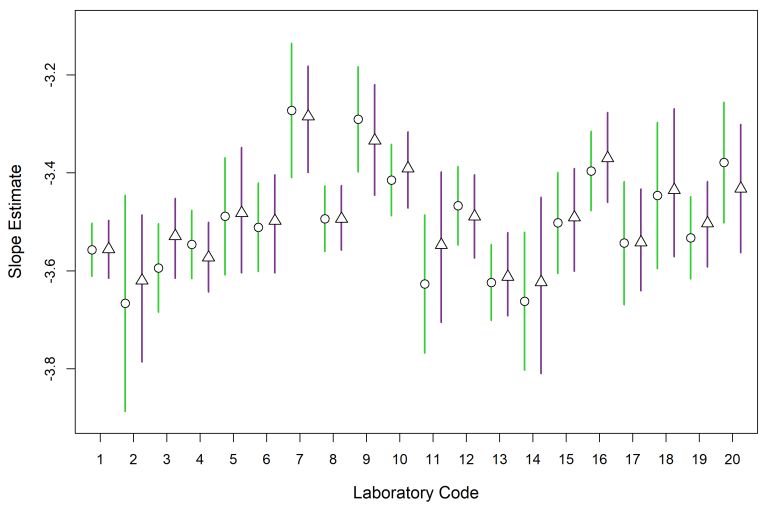
Water 2020, 12, 775                                                                                                           7 of 15

      Table 2. Test sample descriptions. Test sample ID’s, type and concentrations as described in Aw et al.,
      [11].

            Test Sample ID            Test Sample Type               Test Sample Concentration(E. coli/100 mL)
                   13                     Ambient                                       86,596
                   14                   Low Dilution                                    20,535
                   15                   High Dilution                                    2371
                   16                     Ambient                                  Not Determined +
                   17                    Low Spike                                       200 *
                   18                    High Spike                                      800 *
        +   Sample E. coli cell concentration not quantified. * Estimated E. coli cell concentration based on spike levels.

2.4.3. Impact of Acceptance Criteria on WLR Intercept and Slope Estimates
     Data from eleven labs were used for this assessment. For ongoing lab composite standard
curve development in 2016–2018, the acceptance criteria were automatically applied to the individual
standard curves by the draft method C Excel workbook. Acceptance criteria included ranges for
intercept (36.66 to 39.25) and slope (−3.23 to −3.74). Additionally, individual passing curves had
to pass an ANCOVA analysis (α = 0.01) as implemented with the Excel workbook. Curves were
generated using data from five standards as described in Sivaganesan et al., [9] however, an additional
sixth standard was also prepared (described in Section 2.2) and analyzed by most labs to extend the
method’s range of quantification. Twenty-one 5-point (using five standards) and nineteen 6-point
(using 6 standards) composite curves were created between 2016 and 2018 and were evaluated for this
portion of the study. The number of individual standard curves analyzed by the different labs each year
varied from four to ten (Table S1). Individual standard curves were used to generate composite 5-point
and 6-point standard curve in two ways: (1) using data from all individual curves without acceptance
criteria screening and (2) using only passing individual curves after acceptance criteria screening
was performed in the workbook. Thus, the number of individual standard curves used to create the
composite curves varied. WLR 5-point and 6-point composite standard curve mean intercept and slope
parameters and 95% CI intervals from the two methods described above were compiled and plotted
separately using R software (V3.6.1) to visually assess the impact of the proposed acceptance criteria.

3. Results

3.1. Bayesian MSC and WLR Standard Curve Model Comparisons
     The goal of these comparisons was to assess whether results from the simpler and more
user-friendly WLR model approximate those from the MSC model and thus can provide a suitable
replacement. All passing individual standard curves analyzed by the twenty-one labs in 2016 had
intercept and slope estimates that passed the ANCOVA test allowing a WLR composite standard curve
to be produced for every lab. However, lab code 21 was excluded from the model comparisons since it
was not used in the Bayesian MSC analysis [9].
     Estimates of the mean intercepts and the corresponding 95% CI and BCI calculated from WLR and
Bayesian MSC models were similar for each lab (Figure 1a). Furthermore, the mean values that would
be used in the standard curves from each model were within the uncertainty ranges of the other model
in each case. Similar results were observed for slope values (Figure 1b). Each lab’s mean intercept and
slope, and 95% confidence intervals can be found in Supplementary Table S3.
Water 2020, 12, 775 8 of 15
Water 2020, 12, 775 8 of 15
(a)
(b)
Figure 1.
Figure 1. Weighted
Weighted Linear
Linear Regression
Regression (WLR)
(WLR) and
and Master
Master Standard
Standard Curve
Curve (MSC)
(MSC) mean
mean intercept
intercept and
and
slope estimates.
slope estimates. Comparison of (a) mean intercept and (b) slope estimates of the 2016 standard curve
standard curve
composite WLR (green bar with open
composite open circle) and
and Bayesian
Bayesian MSC (purple bar with open triangles)
models. Open circles and triangles on bars indicate the mean least-squares and Bayesian
models. Bayesian intercept
intercept and
and
slope estimates,
slope estimates, respectively.
respectively. Vertical
Verticallines
lines represent
represent the
the WLR
WLR 95%
95% CI
CI (green)
(green) and
and Bayesian MSC 95%
BCI (purple).
BCI (purple).
3.2.
3.2. Comparison
Comparison of
of Test
Test Sample
Sample E.
E. coli
coli Estimates
Estimates by
by the
the Two
TwoModels
Models
The
The goal
goal of
of this
this analysis
analysis was
was to
to examine
examine the
the effects
effects of
of the
the two
two models
models onon mean test sample
mean test sample E.E.
coli estimates (Supplementary Table S4) and the between-lab variability of these estimates.
coli estimates (Supplementary Table S4) and the between-lab variability of these estimates. The mean The mean
estimates
estimatesof ofE.E.coli
colilog 1010target
log gene
target copies
gene from
copies the the
from different labs labs
different werewere
highly overlapping
highly for all for
overlapping water
all
samples using the standard curve intercept and slope values from the two models
water samples using the standard curve intercept and slope values from the two models (Figure 2).(Figure 2).Water 2020, 12, 775 9 of 15
Water 2020, 12, 775 9 of 15
Figure
Figure 2.
2. Test sample E.
Test sample E. coli
coli target
target gene
gene copy
copy results. Green circles
results. Green circles (WLR)
(WLR) and purple triangles
and purple triangles (MSC)
(MSC)
represent E. coli concentrations quantified with the two models. X-axis is the test sample identification
represent E. coli concentrations quantified with the two models. X-axis is the test sample identification
number.
number. Y-axis
Y-axis is
is the
themean
meanlog log10 E. coli copies per reaction.
10 E. coli copies per reaction.
3.3. Impact of Acceptance Criteria on WLR Intercept and Slope Estimates
3.3. Impact of Acceptance Criteria on WLR Intercept and Slope Estimates
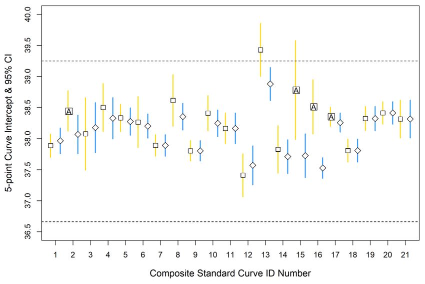
For ongoing sample analyses in 2016–2018, each individual curve’s intercept was required to meet
For ongoing sample analyses in 2016–2018, each individual curve’s intercept was required to
the intercept and slope acceptance criteria in addition to passing ANCOVA analysis, as described in
meet the intercept and slope acceptance criteria in addition to passing ANCOVA analysis, as
Section 2.4.3, before the development of composite curves. The impact of imposing the acceptance
described in Section 2.4.3, before the development of composite curves. The impact of imposing the
criteria, including the ANCOVA, on five-point individual standard curves was examined by visually
acceptance criteria, including the ANCOVA, on five-point individual standard curves was examined
assessing the variability in composite standard curve mean intercept and slope values before and
by visually assessing the variability in composite standard curve mean intercept and slope values
after screening using the above criteria. When acceptance criteria were not imposed, there were four
before and after screening using the above criteria. When acceptance criteria were not imposed, there
instances of intercept and three instances of slope values where the individual curves did not pass the
were four instances of intercept and three instances of slope values where the individual curves did
ANCOVA (Figure 3a,b). In contrast, when only passing individual standard curves were analyzed,
not pass the ANCOVA (Figure 3a and b). In contrast, when only passing individual standard curves
there were no instances of a failing ANCOVA. In one instance, the five-point composite standard curve
were analyzed, there were no instances of a failing ANCOVA. In one instance, the five-point
mean intercept value fell outside the global acceptance range (standard curve 13; Figure 3a) when
composite standard curve mean intercept value fell outside the global acceptance range (standard
individual standard curves were used without acceptance criteria screening but was within the global
curve 13; Figure 3a) when individual standard curves were used without acceptance criteria
acceptance range when individual curves were screened. No composite curve intercept or slope 95 %
screening but was within the global acceptance range when individual curves were screened. No
CI from individual standard curves passing the acceptance criteria fell outside the global acceptance
composite curve intercept or slope 95 % CI from individual standard curves passing the acceptance
ranges. The 95 % CIs also were often narrower for composite curve intercept and slope values when
criteria fell outside the global acceptance ranges. The 95 % CIs also were often narrower for composite
generated from passing individual standard curves compared to when the acceptance criteria were not
curve intercept and slope values when generated from passing individual standard curves compared
used to screen the curves.
to when the acceptance criteria were not used to screen the curves.
Individual and composite standard curve intercept and slope estimates using the sixth standard
with a lower quantity of target sequences (six-point curves) were also evaluated during ongoing
analyses in 2016–2018. Results were not available for curves 2 and 21 because the sixth standard was
not analyzed by that lab; and for curve 15 because there were insufficient passing individual standard
curves to perform the ANCOVA analysis (Figure 4). Three intercept and two slope values of composite
curves generated from unscreened individual standard curves did not pass the ANCOVA. Composite
curve intercept values from individual curves that passed the screening failed the ANCOVA four
times and the slope value failed once. In all instances except one (Figure 4b, curve 5), the composite
curve mean intercept and slope values and their 95% CIs fell within the global acceptance range of the
proposed criteria when the individual standard curves were screened and, as was observed for theWater 2020, 12, 775 10 of 15
five-point curve results, the 95% CI ranges were often narrower for composite curves generated from
only acceptable individual standard curves. The mean intercept and slope, and their lower and upper
bounds of the five-point and six-point composite curves, before and after data were screened with
acceptance
Water 2020, 12,criteria
775 are presented in Supplementary Table S5. 10 of 15
(a)
(b)
Figure 3.
Figure 3. Mean 5-point composite standard curves intercept
intercept and
and slope
slope estimates
estimates and
and 95
95 %% confidence
confidence
intervals (CIs).
intervals (CIs). (a) Mean intercept; and (b) mean slope estimates before (open squares with gold lines)
and after
and after(open
(opendiamonds
diamonds with
with blueblue lines)
lines) data data screening
screening with
with the the proposed
proposed acceptance
acceptance criteria.
criteria. Vertical
Vertical
lines lines represent
represent 95% CIs. Horizontal
95% CIs. Horizontal dashed lines dashed lines
represent therepresent
standard the standard
curve curve
acceptance acceptance
criteria range.
criteria range. Boxes with an inset “A” show individual standard curves without acceptance
Boxes with an inset “A” show individual standard curves without acceptance criteria enforced that did criteria
enforced
not pass thethat did notofpass
analysis the analysis
covariance of covariance
(ANCOVA) therefore(ANCOVA)
a compositetherefore a composite
curve value curve value
was not calculated in
wasExcel
the not calculated
workbook.in the Excel workbook.
Individual and composite standard curve intercept and slope estimates using the sixth standard
with a lower quantity of target sequences (six-point curves) were also evaluated during ongoing
analyses in 2016–2018. Results were not available for curves 2 and 21 because the sixth standard was
not analyzed by that lab; and for curve 15 because there were insufficient passing individual standard
curves to perform the ANCOVA analysis (Figure 4). Three intercept and two slope values of
composite curves generated from unscreened individual standard curves did not pass the ANCOVA.
Composite curve intercept values from individual curves that passed the screening failed theacceptance range of the proposed criteria when the individual standard curves were screened and,
as was observed for the five-point curve results, the 95% CI ranges were often narrower for composite
curves generated from only acceptable individual standard curves. The mean intercept and slope,
and their
Water lower
2020, 12, 775 and upper bounds of the five-point and six-point composite curves, before and
11after
of 15
data were screened with acceptance criteria are presented in Supplementary Table S5.
(a)
(b)
Figure 4.
Figure 4. Mean
Mean 6-point
6-point composite
composite standard
standard curves
curves intercept and slope
intercept and slope estimates
estimates and
and 95%
95% (confidence
(confidence
intervals) CIs. (a) Mean intercept; and (b) Mean slope estimates before data screening
intervals) CIs. (a) Mean intercept; and (b) Mean slope estimates before data screening (open squares (open squares
with gold
with goldlines)
lines)
andand after
after (open(open diamonds
diamonds withlines).
with blue blue Vertical
lines). lines
Vertical lines 95%
represent represent 95% CIs.
CIs. Horizontal
Horizontal
dashed linesdashed linesthe
represent represent
standard thecurve
standard curve acceptance
acceptance criteria
criteria range. range.
Boxes withBoxes with‘A’
an inset anshow
inset
‘A’ show individual
individual standard
standard curves curvesacceptance
without without acceptance criteriathat
criteria enforced enforced that
did not didthe
pass notANCOVA
pass the
ANCOVA
therefore a therefore
compositeacurvecomposite
valuecurve
would value would
not be not be calculated;
calculated; the box with theanbox with
inset ‘B’ an insetindividual
shows ‘B’ shows
individualcurves
standard standard
that curves that were
were screened screened
with with acceptance
acceptance criteria andcriteria andanalysis
failed the failed the analysis of
of covariance
covariance (ANCOVA);
(ANCOVA); the box with an theinset
box ‘C’
with an inset
indicates ‘C’ indicates
an insufficient an insufficient
number number ofstandard
of passing individual passing
individual
curves standard
to generate curves to generate
a composite curve; and a composite
boxes withcurve; and
an inset boxes
‘D’, withwas
no data an inset ‘D’, no data was
collected.
collected.
4. Discussion and Conclusions
4. Discussion and Conclusions
4.1. WLR and Bayesian MSC Standard Curve Model Comparisons
4.1. WLR
This and Bayesiancompared
assessment MSC Standard Curve Model
two standard curveComparisons
models: a simplified WLR model that is currently
being used in a draft method C Excel workbook; and the Bayesian MSC model that was previously
used to define the variability of draft method C results in a large multi-lab study [11]. While different
approaches were used to determine the uncertainty ranges of the intercept and slope estimates from the
two models: 95% CI for WLR; and 95% BCI for MSC, the magnitude of these ranges was the same or
similar in most instances and the ranges were highly overlapping for all labs (Figure 1, SupplementaryWater 2020, 12, 775 12 of 15
Table S4). Consistent with these observations, the mean intercept and slope estimates from the two
models were also highly similar for each of the labs. Given that only the mean intercept and slope
estimates are used for the quantification of test samples in draft method C, it is significant that the
mean values from each model were always within the uncertainty ranges of the other model for each of
the labs. These results suggest that E. coli target gene copies in test samples that are based on standard
curves generated by the WLR and MSC models will not show meaningful differences, thus providing
preliminary evidence to support the use of the WLR model as an adequate approximation of the MSC
model for standard curve development.
4.2. Comparison of Test Sample E. coli Estimates by the Two Models
Estimates of E. coli target gene copies from standard curve-based qPCR methods are dependent
on both the intercept and slope variables. Therefore, our independent comparisons of the intercept and
slope estimates from the WLR and MSC models do not fully predict the similarity of test sample results
that the two models would produce, nor do they reflect the performance of the workbook’s WLR
model in ongoing studies by the labs. To further address these questions, mean intercept and slope
values determined from the MSC model in the 2016 study and corresponding, selected WLR values
generated by the same labs from analyses of the same standards in subsequent studies in 2016–2018
were used to determine estimates of target gene copies in test samples from the 2016 study using
the same test sample measurement data from the 2016 study in each case. Because the target gene
copy estimates obtained from the MSC and WLR standard curves incorporated the differences in both
intercept and slope values from the two models and used ongoing 2016–2018 WLR curves for each lab,
the highly overlapping results among the different labs for each sample provided further support for
adopting the WLR model in the workbook for ongoing standard curve development.
4.3. Impact of Acceptance Criteria on WLR Intercept and Slope Estimates
Quantification of E. coli by qPCR requires a standard curve model and variation and error can be
introduced during each step of the analysis [15]. Factors such as storage time, storage temperature
of standards and reagents, precision of dilutions, and pipette calibration can influence the accuracy
of standard concentration measurements used to create the standard curve [8,16]. Additionally,
differences in equipment used within and between laboratories as well as the ability of analysts to
pipette uniformly contribute to variations in the individual standard curves. One way to reduce
variation is by imposing quality control procedures, such as standard curve acceptance criteria, to help
ensure results generated by different labs are maintained within a defined range.
When individual curves were not screened, the mean intercept and slope values of the composite
curves still fell within the acceptance ranges in most cases, however, the 95% CIs frequently extended
outside. The mean intercept and slope values of the 5-point composite curves as well as their 95%
CIs consistently fell within the proposed acceptance ranges when individual curves from ongoing
studies in 2016–2018 were screened. Furthermore, 95% CIs were equal or narrower for most five-point
composite standard curves after screening individual curves. The narrower intervals generated after
screening suggest less uncertainty in the mean parameter values.
ANCOVA analysis also was performed on the individual curves comprising each five- or six-point
composite curve in the workbook. Intercept and slope values of the individual standard curves cannot
be significantly different for the Method C workbook to generate composite curves. Several of the
five-point composite curves failed the ANCOVA analysis when the individual curves were not screened,
however, all five-point composite curves passed when the individual curves were screened with the
intercept and slope acceptance criteria. In contrast, several six-point composite curves failed ANCOVA
analyses even after screening individual curves with the acceptance criteria. Six-point standard
curves have been successfully used to extend the draft method C quantification range for developing
relationships between qPCR and culture data (R. Haugland, personal communication) but their use is
not presently considered to be essential for routine beach monitoring. The increased ANCOVA failureWater 2020, 12, 775 13 of 15
rate of six-point curves among the labs after screening could be related to the decentralized preparation
of the sixth standard by each lab and thus may highlight previous recommendations that reference
DNA be verified and provided by a single supplier [9,17].
4.4. Draft Method C Implementation
Although the MSC model can provide a better understanding of the sources of uncertainty in
these estimates [8], the results of this study suggest that the use of the WLR model will have little
effect on the determination of mean estimates of E. coli target gene copies in test samples in draft
method C. As such, the WLR model incorporated into the Excel workbook can be expected to provide
a reliable but simpler alternative to the MSC model for recreational water testing by draft method C.
Our results further suggest that the automatic incorporation of individual and composite standard
curve acceptance criteria in the workbook may reduce the uncertainty of quantifying E. coli target
gene copy estimates in some instances and at least should provide greater consistency in the results.
Largely due to resource limitations by many end-user labs, characterizing the uncertainty of test sample
estimates is not presently a priority in draft method C implementation for beach monitoring. However,
it could be important for other applications of the method and this issue has been addressed in recent
U.S. EPA microbial source tracking (MST) methods [10].
Use of either a composite WLR or a Bayesian MSC model in place of individual standard curves
on each reaction plate, which is typical of many qPCR methods [10,18,19], increases sample analysis
efficiency, reduces the costs of preparing or purchasing standards and increases the number of test
samples that can be analyzed on each plate. A previous report [16] suggested that the use of master (or
composite) curves may be most efficient for studies involving large numbers of continuous sample
analyses over time, which may be typical for beach monitoring programs, while generating standard
curves on each reaction plate may be more suitable for smaller-scale or more sporadic analyses which
could be the case for many MST studies. However, it is also recognized that care must be taken when
applying master or composite standard curves to test sample data from multiple plate runs. This issue
is partially addressed in draft method C by the analyses of positive control samples on each plate.
Acceptance criteria for these analysis results were also established in the 2016 multi-lab study [9,11] and
are incorporated into the draft method C workbook. Beyond this, guidance also has been established
for labs implementing draft method C wherein the minimum quantity of four acceptable individual
standard curves, used for composite curve development, should be obtained from a maximum of six
independent curve runs. With the incorporation of some flexibility into this guidance, e.g., curves
where known or suspected technical or logistical issues have been identified can be ignored, all the labs
performing ongoing recreational water sample analyses in 2016–2018 using draft method C (Table 1)
were able to meet this basic minimum requirement with their five-point curves.
Our findings support the use of draft method C with the Excel workbook and proposed acceptance
criteria as a rapid, standardized protocol for estimating E. coli densities in recreational waters. The Excel
workbook, WLR calculation, and acceptance criteria will help public laboratories and scientists perform
draft method C in an efficient and cost-effective manner that produces reliable data.
Supplementary Materials: The following are available online at http://www.mdpi.com/2073-4441/12/3/775/s1,
Table S1: Number of standard curves analyzed by each lab, Table S2: Intercept and slope 95% Bayesian MSC
Credible Intervals, Table S3: Mean intercept and slope values from Weighted Linear Regression (WLR) by lab, Table
S4: Test sample E. coli estimates, Table S5: Mean intercept and slope before and after data screening; Microsoft
Excel Workbook: Method C Workbook.
Author Contributions: The following statements should be used “conceptualization, R.H., M.S.; methodology,
M.S., R.H., J.N.M.; software, J.N.M. and M.J.L.; validation, all authors; formal analysis, J.N.M., M.J.L.; data curation,
R.H., M.L.; writing—original draft preparation, M.L., J.M., and R.R.R.; writing—review and editing, All authors;
supervision, R.H.; project administration, R.H., S.B.; funding acquisition, S.B., R.R.R.”. All authors have read and
agreed to the published version of the manuscript.
Funding: This research was funded by the following: The State of Michigan through the Real-time Beach
Monitoring Program, multiple years; The Michigan Department of Environment, Great Lakes, and Energy (EGLE),
grant number 2018-7214.Water 2020, 12, 775 14 of 15
Acknowledgments: We would like to thank all personnel from participating labs for dedicating their time to this
study. Information has been subjected to U.S. EPA peer and administrative review and has been approved for
external publication. Any opinions expressed in this paper are those of the authors and do not necessarily reflect
the official positions and policies of the U.S. EPA. Any mention of trade names or commercial products does not
constitute endorsement or recommendation for use.
Conflicts of Interest: The authors declare no conflict of interest and the funders had no role in the design of the
study; in the collection, analyses, or interpretation of data; in the writing of the manuscript, or in the decision to
publish the results”.
References
1. Health Effects Criteria for Fresh Recreational Waters. Available online: https://permanent.access.gpo.gov/
lps68259/frc.pdf (accessed on 8 March 2020).
2. Wade, T.J.; Calderon, R.L.; Sams, E.; Beach, M.; Brenner, K.P.; Williams, A.H.; Dufour, A.P. Rapidly Measured
Indicators of Recreational Water Quality Are Predictive of Swimming-Associated Gastrointestinal Illness.
Environ. Health Perspect. 2006, 114, 24–28. [CrossRef] [PubMed]
3. Department of Environmental Quality. Michigan Public Health Code Part 4. Water Quality Standards.
Available online: https://www.michigan.gov/documents/deq/wrd-rules-part4_521508_7.pdf (accessed on 7
November 2019).
4. Recreational Water Quality Criteria. Available online: https://www.epa.gov/sites/production/files/2015-10/
documents/rwqc2012.pdf (accessed on 30 October 2019).
5. Lavender, J.S.; Kinzelman, J.L. A Cross Comparison of QPCR to Agar-Based or Defined Substrate Test
Methods for the Determination of Escherichia Coli and Enterococci in Municipal Water Quality Monitoring
Programs. Water Res. 2009, 43, 4967–4979. [CrossRef]
6. Pfaffl, M.W.; Hageleit, M. Validities of mRNA Quantification Using Recombinant RNA and Recombinant
DNA External Calibration Curves in Real-time RT-PCR. Biotechnol. Lett. 2001, 23, 275–282. [CrossRef]
7. Rutledge, R.G. Mathematics of Quantitative Kinetic PCR and the Application of Standard Curves. Nucleic
Acids Res. 2003, 31, e93. [CrossRef] [PubMed]
8. Sivaganesan, M.; Seifring, S.; Varma, M.; Haugland, R.A.; Shanks, O.C. A Bayesian Method for Calculating
Real-Time Quantitative PCR Calibration Curves Using Absolute Plasmid DNA Standards. BMC Bioinf. 2008,
9, 120. [CrossRef] [PubMed]
9. Sivaganesan, M.; Aw, T.G.; Briggs, S.; Dreelin, E.; Aslan, A.; Dorevitch, S.; Shrestha, A.; Isaacs, N.; Kinzelman, J.;
Kleinheinz, G.; et al. Standardized Data Quality Acceptance Criteria for a Rapid Escherichia Coli QPCR
Method (Draft Method C) for Water Quality Monitoring at Recreational Beaches. Water Res. 2019, 156,
456–464. [CrossRef] [PubMed]
10. Shanks, O.C.; Kelty, C.A.; Oshiro, R.; Haugland, R.A.; Madi, T.; Brooks, L.; Field, K.G.; Sivaganesan, M. Data
Acceptance Criteria for Standardized Human-Associated Fecal Source Identification Quantitative Real-Time
PCR Methods. Appl. Environ. Microbiol. 2016, 82, 2773–2782. [CrossRef] [PubMed]
11. Aw, T.G.; Sivaganesan, M.; Briggs, S.; Dreelin, E.; Aslan, A.; Dorevitch, S.; Shrestha, A.; Isaacs, N.;
Kinzelman, J.; Kleinheinz, G.; et al. Evaluation of Multiple Laboratory Performance and Variability in
Analysis of Recreational Freshwaters by a Rapid Escherichia Coli QPCR Method (Draft Method C). Water Res.
2019, 156, 465–474. [CrossRef] [PubMed]
12. Chern, E.C.; Siefring, S.; Paar, J.; Doolittle, M.; Haugland, R.A. Comparison of Quantitative PCR Assays for
Escherichia Coli Targeting Ribosomal RNA and Single Copy Genes. Lett. Appl. Microbiol. 2011, 52, 298–306.
[CrossRef] [PubMed]
13. Sivaganesan, M.; Varma, M.; Siefring, S.; Haugland, R. Quantification of Plasmid DNA Standards for U.S.
EPA Fecal Indicator Bacteria QPCR Methods by Droplet Digital PCR Analysis. J. Microbiol. Methods 2018,
152, 135–142. [CrossRef] [PubMed]
14. Cook, R.D.; Weisberg, S. Diagnostics for Heteroscedasticity in Regression. Biometrika 1983, 70, 1–10. [CrossRef]
15. Baker, M. QPCR: Quicker and Easier but Don’t Be Sloppy. Nat. Methods 2011, 8, 207–212. [CrossRef]
16. Sivaganesan, M.; Haugland, R.A.; Chern, E.C.; Shanks, O.C. Improved Strategies and Optimization of
Calibration Models for Real-Time PCR Absolute Quantification. Water Res. 2010, 44, 4726–4735. [CrossRef]
[PubMed]Water 2020, 12, 775 15 of 15
17. Shanks, O.C.; Sivaganesan, M.; Peed, L.; Kelty, C.A.; Blackwood, A.D.; Greene, M.R.; Noble, R.T.; Bushon, R.N.;
Stelzer, E.A.; Kinzelman, J.; et al. Interlaboratory Comparison of Real-Time Pcr Protocols for Quantification
of General Fecal Indicator Bacteria. Environ. Sci. Technol. 2012, 46, 945–953. [CrossRef] [PubMed]
18. Converse, R.R.; Blackwood, A.D.; Kirs, M.; Griffith, J.F.; Noble, R.T. Rapid QPCR-Based Assay for Fecal
Bacteroides Spp. as a Tool for Assessing Fecal Contamination in Recreational Waters. Water Res. 2009, 43,
4828–4837. [CrossRef] [PubMed]
19. Noble, R.T.; Blackwood, A.D.; Griffith, J.F.; McGee, C.D.; Weisberg, S.B. Comparison of Rapid Quantitative
PCR-Based and Conventional Culture-Based Methods for Enumeration of Enterococcus Spp. and Escherichia
Coli in Recreational Waters. Appl. Environ. Microbiol. 2010, 76, 7437–7443. [CrossRef] [PubMed]
© 2020 by the authors. Licensee MDPI, Basel, Switzerland. This article is an open access
article distributed under the terms and conditions of the Creative Commons Attribution
(CC BY) license (http://creativecommons.org/licenses/by/4.0/).You can also read