Fast Iterative Five point Relative Pose Estimation
←
→
Page content transcription
If your browser does not render page correctly, please read the page content below
Fast Iterative Five point Relative Pose
                        Estimation

                             Johan Hedborg and Michael Felsberg

                            Linköping University Post Print

                     N.B.: When citing this work, cite the original article.

©2013 IEEE. Personal use of this material is permitted. However, permission to
reprint/republish this material for advertising or promotional purposes or for creating new
collective works for resale or redistribution to servers or lists, or to reuse any copyrighted
component of this work in other works must be obtained from the IEEE.

Johan Hedborg and Michael Felsberg, Fast Iterative Five point Relative Pose Estimation,
2013, IEEE Workshop on Robot Vision.

Postprint available at: Linköping University Electronic Press
            http://urn.kb.se/resolve?urn=urn:nbn:se:liu:diva-90102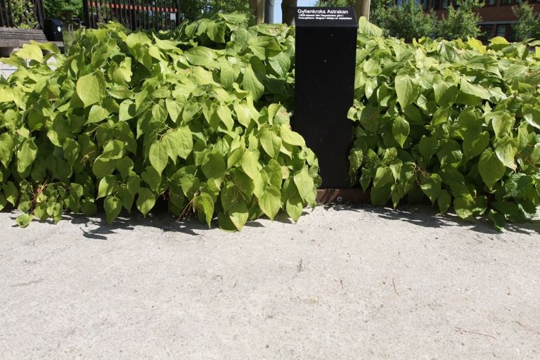
Fast Iterative Five point Relative Pose Estimation

                                            Johan Hedborg Michael Felsberg
                                               Computer Vision Laboratory
                                              Linköping University, Sweden
                                               https://www.cvl.isy.liu.se/

                         Abstract                                      the respective epipolar lines. By minimizing an error based
                                                                       on the epipolar distance instead of an error in 3D space, no
   Robust estimation of the relative pose between two cam-             structure estimation is required, thus leading to fewer un-
eras is a fundamental part of Structure and Motion meth-               known parameters and to a significant reduction in calcula-
ods. For calibrated cameras, the five point method together            tions.
with a robust estimator such as RANSAC gives the best re-
sult in most cases. The current state-of-the-art method for            1.1. Related work
solving the relative pose problem from five points is due to               In the case of calibrated cameras, the pose estimation
Nistér [9], because it is faster than other methods and in the        problem is most accurately solved using the minimal case
RANSAC scheme one can improve precision by increasing                  of five points within a robust estimator (RANSAC) frame-
the number of iterations.                                              work, [9, 17, 12]. The five point problem is a well un-
   In this paper, we propose a new iterative method, which             derstood topic and there exists a wide variety of solutions.
is based on Powell’s Dog Leg algorithm. The new method                 Among the first methods is the early work by [2] and more
has the same precision and is approximately twice as fast as           recent work can be found in [7, 18].
Nistér’s algorithm. The proposed method is easily extended
                                                                           As a consequence of using the five point solver within a
to more than five points while retaining a efficient error met-
                                                                       RANSAC loop, the speed of the solver is of great practical
rics. This makes it also very suitable as an refinement step.
                                                                       relevance because the accuracy can be improved by using
   The proposed algorithm is systematically evaluated on
                                                                       more iterations, [5]. Therefore, the current state-of-the-art
three types of datasets with known ground truth.
                                                                       method is due to Nistér [9], as his method is capable of cal-
                                                                       culating the relative pose within a RANSAC loop in video
                                                                       real-time. However, to achieve this level of performance, a
1. Introduction                                                        considerable implementation effort is required, [7].
   The estimation of the relative position and orientation                 Stewénius [18] improved the numerical stability of [9]
of two cameras based on the image content exclusively is               by using Gröbner bases to solve a series of third order poly-
the basis for a number of applications, ranging from aug-              nomials instead of solving a tenth order polynomial. How-
mented reality to navigation. In many cases, it is possible            ever, this gain in stability comes with a performance penalty
to estimate the intrinsic parameters of the camera prior to            due to a 10x10 eigenvector decomposition.
the pose estimation. This reduces the number of unknowns                   An alternative to algebraic solvers are non-linear op-
to five. This particular case is the problem considered in             timization methods, which find the solution iteratively,
this paper and the current state-of-the-art solution is the five       e.g. using the Gauss-Newton method, [14]. However, the
point solver presented by Nistér [9] combined with a pre-             Gauss-Newton method becomes unstable if the Hessian is
emptive scoring scheme, [10], in a RANSAC loop, [3].                   ill-conditioned. To compensate for that the authors pro-
   We propose to solve the five point problem iteratively              pose to include more than five points in the estimation of
using Powell’s Dog Leg (DL) method, [11]. We show that                 the pose, [14], section 4.2. The speed reported in [14] is
a non-linear DL solver with five parameters is faster than             prohibitively slower (about four orders of magnitude) than
the currently fastest five point solver [9]. The DL optimiza-          Nistér’s implementation.
tion method is a commonly used method for solving general                  In terms of evaluation, many authors have been using
non-linear systems of equations and least square problems.             synthetic data in order to have access to ground truth infor-
   Our formulation of the five point problem is based on               mation, [9, 18, 12]. Using additive Gaussian noise in these
the epipolar distance, [5], i.e. the distance of the points to         synthetic datasets does not necessarily lead to realistic eval-

                                                                   1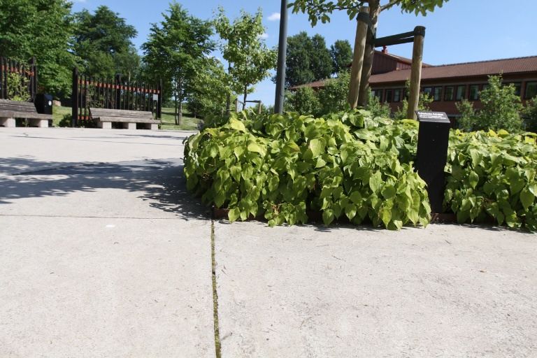
uation results. 2.2. Essential matrix estimation problem
1.2. Main contributions Equation 5 allows us to verify whether the image points
and the essential matrix are consistent, but in practice we
The main contributions of this paper are: need to estimate E from sets of points. Usually, these sets
• We propose a new iterative method for solving the five of points contain outliers and to obtain a robust estimate,
point relative pose problem using the Dog Leg algo- one usually uses RANSAC. Within the RANSAC loop, it is
rithm. preferable to use as few points as possible, [3]. The min-
• The new method is nearly a factor of two faster and at imum number of points is determined by the degrees of
least as accurate as the current state-of-the-art. freedom in E = R[t]× as (5) gives us one equation per
• We demonstrate the methods ability to generalize to correspondence. Hence we need five points.
more than five points and the increase in precision. The degrees of freedom also determine the dimension-
• We provide a novel type of dataset consisting of real ality of minimal parameterizations. For reasons of com-
image sequences and high accuracy ground truth cam- putational efficiency, we chose a parametrization with five
era poses (throw the authors homepage). angles w = [α β γ θ φ], further details are given in
The remainder of the paper is structured as follows. In Appendix A.
the subsequent section, we formalize the relative pose esti- Given five points, we aim at computing E(w) using an
mation problem and introduce our novel algorithm. In sec- iterative solver of non-linear systems of equations instead
tion three we describe the evaluation and in section four we of a closed form solution. For this purpose, we need to have
present and analyze the results. geometric error rather than a purely algebraic one. One pos-
sibility to define a geometric error is in terms of the distance
2. Methods between a point in one view xi and the epipolar line li from
the corresponding point x′i in the other view, [5]:
2.1. Problem formulation
ri (w) = li (w)xi , (6)
A 3D world point xw i is projected onto two images, re-
sulting in two corresponding image points xi and x′i . The where
T
projections are defined by x′ i E(w)
li (w) = (7)
||x i e1 (w) x′ Ti e2 (w)||2
′ T
xi ∼ P1 x w
i , P1 = K1 [I|0] (1)
and ej (w) are the column vectors of E(w). Note that the
x′i ∼ P2 x w
i , P2 = K2 [R12 |t12 ] , (2) symmetric variant of (6) is the Sampson distance, [13].
where ∼ denotes equality up to scale and the first camera Hence, we want to solve
defines the coordinate system.
r1 (w∗ )
Let R12 and t12 denote the rotation and the translation
r(w∗ ) = ... = 0 (8)
between camera 1 and 2. The cameras are related as, [2],
r5 (w∗ )
′T T
x K−1
2 EK−1
1 x =0 , (3)
and w∗ is a global minimizer of
where E = R12 [t12 ]× is the essential matrix, which con- 1
tains the relative rotation and translation between the views. σ(w) = ||r(w)||22 . (9)
2
The translation [tx ty tz ] is represented as a skew symmet-
ric cross product matrix 2.3. Iterative solution using Dog Leg
Equation 9 can be categorized as a non-linear least
0 −tz ty
squares problem, and solved by e.g. the Gauss-Newton
[t12 ]× = tz 0 −tx . (4)
method, [14]. We have instead chosen to apply an alter-
−ty tx 0
native method that combines Newton-Raphson (NR) and
If the internal camera parameters K1 , K2 are known, we steepest descent (SD), called Dog Leg (DL), because ”The
can assume that the image points are rectified, i.e. , they are Dog Leg method is presently considered as the best method
multiplied beforehand by K−1 −1
1 and K2 , respectively. In
for solving systems of non-linear equation.” [8]
that case, (3) becomes The combination of NR and SD is determined by means
of the radius ∆ of a trust region. Within this trust region,
T
x′ Ex = 0 . (5) we assume that we can model r(w) locally using a linear
model ℓ :
To simplify notation, we omit the subindex ·12 for the rota-
tion R and the translation t in what follows. r(w + h) ≈ ℓ (h) , r(w) + J(w)h , (10)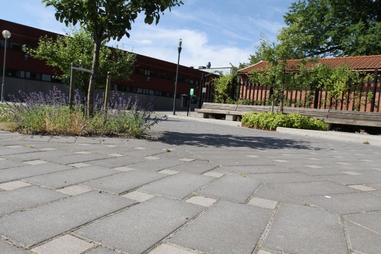
∂r         ∂r
where J = [ ∂w  1
                  . . . ∂w 5
                             ] is the Jacobian.                   are data independent and can easily be implemented on a
    The Newton-Raphson update hnr is obtained by solving          parallel computer, e.g. GPU.
J(w)h = −r(w) e.g. by Gauss elimination with pivoting.                There are some further parameters in the DL algorithm
If the update is within the trust region (khnr k2 ≤ ∆), it is     that have to be chosen. ∆0 is the start value for ∆, which is
used to compute a new potential parameter vector                  set to 1 in our implementation. An upper limit of the num-
                                                                  ber of iterations is defined to avoid a waste of computational
                     wnew = w + hnr .                     (11)    power in cases of that do not converge. In these cases, the
   Otherwise, compute the gradient g = JT r and the steep-        resulting pose estimate is usually inaccurate and will be ne-
est descent step hsd = −αg (for the computation of the step       glected anyway. We use an upper limit 5 for the number of
length α, see Appendix B). If the SD step leads outside the       iterations for DLinit. For DLconst we use a two step strat-
trust region (αkgk2 ≥ ∆), a step in the direction of steepest     egy: for the first 100 iterations the limit set to 8 and then it
descent with length ∆ is applied                                  is lowered to 6. The thresholds for kgk∞ , krk∞ , khk2 , and
                                                                  ∆ are set to 10−9 , 10−9 , 10−10 , and 10−10 , respectively.
                wnew = w − (∆/kgk2 )g .                   (12)
                                                                  2.5. The processing pipeline
   If the SD step is shorter than ∆, β times hnr + αg is
added to produce a vector of length ∆:                                In order to apply the algorithm from the previous section
                                                                  to image sequences, several steps have to be performed be-
            wnew = w − αg + (hnr + αg)β .                 (13)    fore. First of all, we need to calibrate the camera which is
                                                                  done with Zhang’s method, [19]. After this, distinct image
    In all three cases, the new parameter vector is only used
                                                                  regions are extracted using an interest point detector, [15].
in the next iteration (w = wnew ) if the gain factor ρ is posi-
                                                                      We use the KLT-tracker, [15], to obtain point correspon-
tive (for the computation of ρ see Appendix B). Depending
                                                                  dences over time. The KLT-tracker is basically a least-
on the gain factor, the region of trust is growing or shrink-
                                                                  squares matching of rectangular patches that achieves sub-
ing. The iterations are stopped, if kgk∞ , krk∞ , khk2 , or ∆
                                                                  pixel accuracy by gradient search. We use a translation-
is below a threshold or if a maximum number of iterations
                                                                  only model between neighboring frames. Tracking between
is reached.
                                                                  neighboring frames instead of across larger temporal win-
2.4. Initialization                                               dows improves the stability, especially with respect to scale
                                                                  variations that are present in forward motion. When track-
    As with any iterative method, the DL method needs a
                                                                  ing frame-by-frame, the changes in viewing angle and scale
starting point w0 . In the case of pose estimation for video
                                                                  are sufficiently small for tracking to work well. In order to
frames its often possible to quite accurately guess the posi-
                                                                  improve stability of tracked points, the track-retrack (cross-
tion of the next frame, because of physical limitations of
                                                                  check) has been applied in certain cases, [6]. All these
motion (visual odometry). A good prediction is that the
                                                                  steps were performed using Willow Garage’s OpenCV im-
camera motion is constant between frames. To create a
                                                                  plementations.
wider baseline for the pose estimation it is common not
to take subsequent frames but frames further apart. In this
                                                                  3. Evaluation setup
case, the motion until the second but latest frame is already
known and using the prediction described above, a good               We have evaluated our method on three types of data,
starting point for the pose estimation is obtained. This is       consisting of synthetic images, real images and the Notre
meant when referring to DLinit in the Result section.             Dame dataset [16]. Pose estimation methods are com-
    In certain cases, the initial position might be completely    monly tested on synthetic data with added artificial noise,
unknown, e.g. photo sharing sites. The main focus of this         [9, 12, 18, 17]. Since real data might differ significantly
work is however towards real-time video sequences imply-          from synthetic test data, we have also evaluated our method
ing that we have some knowledge of the previous pose. The         on a dataset with real images.
case without prior knowledge is still of occasional interest         The error metric used for our datasets are the difference
i.e. in an initial state or when one loses track resulting in     in angle of the translation direction between the ground
a completely unknown pose. In these cases we obtain con-          truth and the pose estimate. The direction is used because
vergence by first initiating the solver with a standard pa-       of the scale associated with the relative pose estimation is
rameter vector w = 0 (corresponding to a forward motion)          ambiguous. The Notre Dame data set is used to evaluate
for a number of RANSAC iterations. After these first itera-       how well it generalizes to N-points and in order to compare
tions, we initialize the solver with the currently best model     it with the very accurate and fast method of Hartley et al.
(largest RANSAC consensus set). This is referred to as DL-        [4] we use an error metric based on differences in rotation.
const in section 4. The major advantage of DLinit com-               In general, pose estimation methods behave differently
pared to DLconst is that the individual RANSAC iterations         on sideways motion and on forwards motion, [12, 18, 9]. In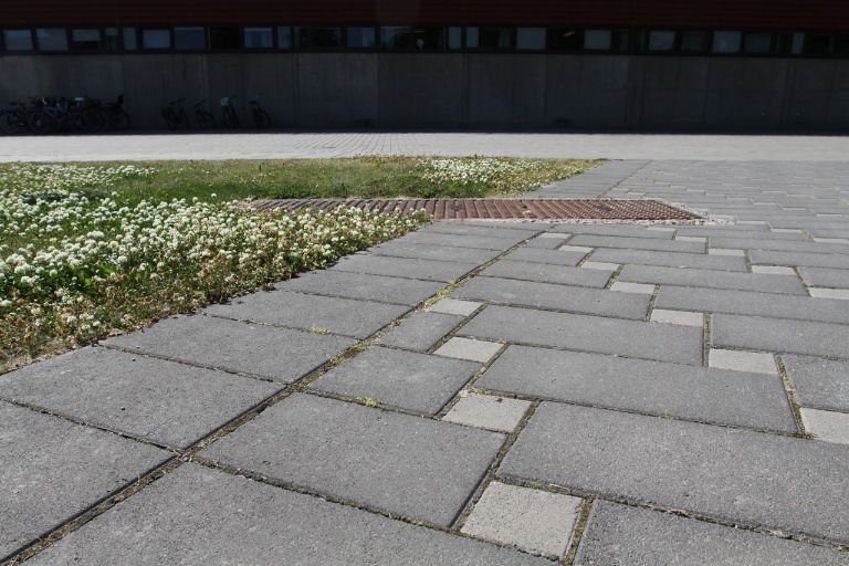
dataset 1 dataset 2 dataset 1 dataset 2
dataset 3 dataset 4 dataset 3 dataset 4
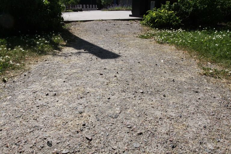
Figure 1. Forward motion, real data. Figure 2. Sideways motion, real data.
order to analyze both cases separately, we have divided the 3.3. The Notre Dame dataset
datasets into two parts, one for forward motion and one for
sideways motion. The full Notre Dame data set consists of 715 images
of 127431 3D points. The number of image pairs with
more than 30 point correspondences are 32051. The dataset
3.1. Synthetic data comes with already reconstructed cameras and points which
has been refined with bundle adjustment. As in [4] we have
We have tested the algorithm on a synthetic dataset,
chosen to use the bundle adjusted cameras as ground truth.
which consists of 1000 randomly positioned 3D world
points viewed by a camera moving both sideways and for-
wards. The world points were projected into the cameras 4. Results
and Gaussian noise (zero mean) was added to the projected
point positions. The noise variance is varied between 0 and The results are presented in Figures. 3-4 as box plots over
1, where standard deviation 1 is equivalent to one pixel in an 500 individual pose estimates. The boxes cover the sec-
image with the size 1024x1024. The horizontal view-angle ond and third quantile and the dots are considered outliers.
is set to 60 ◦ . This follows the methodology used in [9, 18]. Each pose estimate is produced by running a 500 iterations
RANSAC loop.
3.2. Real image sequences All methods are run on the same set of five points,
which is randomly selected before each RANSAC iteration.
The second evaluation dataset is constructed from real Therefore, in the ideal case, all methods should produce
images by applying a methodology motivated by [1]. For the same result for a fixed number of RANSAC iterations.
capturing the images, a 15 megapixel Canon 50D DLSR However, small deviations between the methods occur due
camera has been used, which is capable to capture 6.5 im- to sporadic failures. Failures in Nistér’s method are pre-
ages per second. The relatively low frame rate was com- sumably caused by the preemptive scoring scheme, where
pensated by moving the camera approximately one fourth all solutions are scored using a sixth point and the solution
of the wanted speed. By mounting the camera on a stable with the best score is chosen, [10]. Given that the sixth
wagon and pushing it forward we could get a smooth cam- point is an outlier, a wrong solution is likely to be cho-
era trajectory for the sequence. This allowed us to get ap- sen and a potentially better solution and larger consensus
proximate ground truth for the sequence by estimating the set is potentially disregarded, but with respect to the whole
pose for the high resolution images. A large quantity of RANSAC loop this is still the most efficient solution. The
points has been tracked (∼10K) and the pose has been esti- proposed method occasionally misses the correct solution
mated by using the five point method, [17] within a 10000 due to slow convergence or convergence to another solu-
RANSAC iterations. Examples for the acquired images are tion with the same consequences regarding the consensus
shown in Figure 1 (forward motion) and Figure 2 (sideways set. The failure cases/deviations between the methods can
motion). The dataset images for evaluation are obtained by be observed more frequently in hard cases such as the for-
down-sampling the images to 1 megapixel. ward case with higher amounts of noise.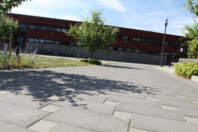
4.1. Synthetic data                                                                                                          Synthetic Scene Sidways 1−4

                                                                                                                Nister
                                                                                                          0.9
   Figure 3 shows the results on synthetic data. We have                                                        DLconst
                                                                                                                DLinit
evaluated all methods on 4 different noise levels with stan-                                              0.8

dard deviation 0.25, 0.50, 0.75, and 1 pixel.

                                                                      translation direction error (deg)
                                                                                                          0.7
   The size of the consensus set depends on the epipolar dis-
                                                                                                          0.6
tance threshold that is used when evaluating the solutions.
In order to get an appropriate fraction of points as inliers,                                             0.5

we need to adjust the threshold according to the noise level.                                             0.4
Without going into further details, the threshold has been
                                                                                                          0.3
scaled linearly with the noise. The noise level can be esti-
mated using e.g. the forward-backward tracking error.                                                     0.2

   According to the box plots, the proposed method per-                                                   0.1
forms nearly identical to the method of Nistér for all
                                                                                                           0
datasets if ti is initialized with the previous camera position                                                 0.25            0.5
                                                                                                                                      Noise level
                                                                                                                                                    0.75   1.0

(DLinit).                                                                                                                    Synthetic Scene Forward 1−4
   One small performance increase can be observed for the                                                       Nister
                                                                                                           4
forward case with large noise and the case of DLconst. This                                                     DLconst
                                                                                                                DLinit
is the hardest case to solve and a high loss of solutions                                                 3.5

during the RANSAC iteration is expected. The increase

                                                                      translation direction error (deg)
                                                                                                           3
of performance of DLconst is probably caused by select-
ing the currently best solution as initialization for the next                                            2.5

RANSAC iteration. However, the improvement is data de-                                                     2
pendent and not statistical significant.
                                                                                                          1.5
4.2. Real image sequences
                                                                                                           1
    In contrast to the synthetic data, the noise level in the
real data is approximately constant and therefore the same                                                0.5

threshold for the epipolar distance is used all cases.                                                     0
                                                                                                                0.25            0.5                 0.75   1.0
    Overall, the accuracy is nearly identical for all methods.                                                                        Noise level
Despite the quite similar performance for the same number
                                                                                                                          Figure 3. Synthetic data
of RANSAC iterations, the DL method is superior in the
way that it is faster than Nistér’s method, see next section.
    Figure 5 shows the difference in precision between             ations are computed, the better precision can be achieved,
Nistér’s and the proposed method. For each RANSAC                 [5]. This is why the method of [9] is still considered to
range of 100 iteration, it shows the error of the currently        be state-of-the-art, even if more accurate methods like [17]
best solution from Nistér’s algorithm minus the error of the      have been proposed later.
currently best solution from our method. Bars in the nega-             Our method is implemented in plain C/C++ code. It is all
tive range indicate that Nistér’s result is more accurate and     compiled and tested on a desktop PC with an Intel 2.66Ghz
bars in the positive range indicate that our results are better.   (W5320) CPU.
As can be seen, in all cases the median error is near zero.            The proposed method is compared with 2 implementa-
Note that the error difference is in the order of 10−6 to 10−8 ,   tions of Nistér’s algorithm, one which is contained in VW34
which is several orders of magnitude smaller than the error        (a library for real-time vision developed at Oxford’s Active
in the pose estimate (about 0.4 degree). Practically speak-        Vision Lab1 ). The second is from Richard Hartley and is to
ing, the methods perform equally well in terms of precision        our knowledge the fastest available implementation 2 .
for the evaluated datasets. One exception is observed for              To accurately compare our method with Nistér’s imple-
the forward motion and DLconst after 100 iterations, where         mentation, we have compiled our code on a Pentium III
one quantile lies significantly below 0 for datasets 3 and 4       desktop PC, with the same type of processor that is used
(not the median though). This is presumably caused by a            in [9]. The performance timings are then compared with
failed initialization using the DLconst strategy.                  the ones found in [9].
4.3. Speed                                                             The average speedups on our data sets are summarized
   The faster the method, the more RANSAC iterations can             1 http://www.robots.ox.ac.uk/ActiveVision/

be computed in the same time. The more RANSAC iter-                  2 http://users.cecs.anu.edu.au/                               hartley/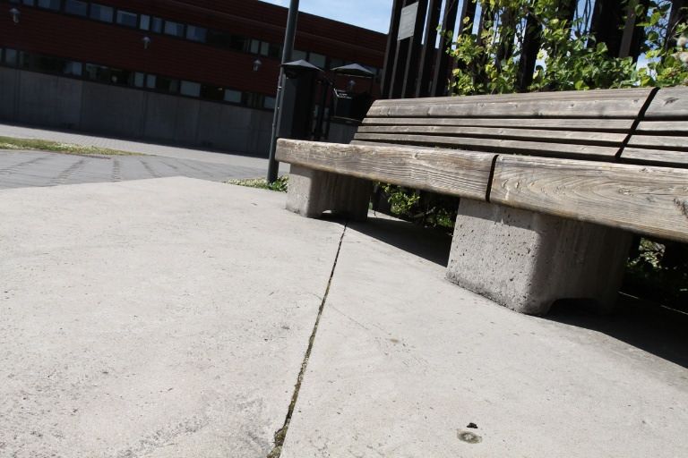
Real Scene Sideways 1−4 −8
x 10 Real data sideways motion, DLinit
2
Nister Dataset 1
DLconst Dataset 2
1.6 1.5
DLinit Dataset 3
Dataset 4
1.4
translation error difference (deg)
translation direction error (deg)
1
1.2
0.5
1
0
0.8
−0.5
0.6
−1
0.4
−1.5
0.2
0 −2
1 2 3 4 100 200 300 400 500
Dataset number Iterations count
Real Scene Forward 1−4 x 10
−7 Real data forward motion, DLconst
2
Nister
0.9
DLconst 1.5
DLinit
0.8
translation error difference (deg)
1
translation direction error (deg)
0.7
0.5
0.6
0.5 0
0.4 −0.5
0.3
−1
0.2
−1.5
0.1
−2
0 100 200 300 400 500
1 2 3 4 Iterations count
Dataset number
Figure 5. The bar plots shows the difference in precision of every
Figure 4. Real data
new best solution found whit in the RANSAC loop. Here we show
the best and the worst case for our method on real data.
Method i7 PIII 550
[9] x 121µs
Nistér(available) 16,5µs x in table 1. For a modern CPU and a currently available
VW34 34.8µs x code we are on average 2-2.5 times faster than the closed
Ours (mean) 7.0µs 72.1µs form solution. Compared with Nistér’s own implementation
on older hardware, we achieve an average speedup between
Table 1. Timings for different methods and implementations. The 1.5x and 1.9x.
time for our method is the mean over all tested datasets.
4.4. N-point generalization
Data type time Nistér(paper) Nistér(imp)
The approach in section 2.3 allows us to use more then
Realdata DLconst 7.5µs 1.6x 2.2x five points to solve the relative pose, with very minor
Realdata DLinit 6.5µs 1.9x 2.5x changes to the actual implementation. Instead of solving
Syntdata DLconst 7.7µs 1.5x 2.1x the square linear equation (LSQ) system J(w)h = −r(w)
Syntdata DLinit 7.1µs 1.7x 2.3x arising from (10), we need to solve the alternative LSQ
system J(w)T J(w)h = −J(w)T r(w) (a.k.a. the normal
Table 2. Average timings for each of the real and synthetic
datasets, using DLconst and DLinit. The Nistér(paper) column equations). This and the fact that the residual is defined
is the speed up compared with [9] on the PIII and Nistér(imp) is as an reprojection error (line to point distance in image),
the implementation freely available from Hartley renders our method an interesting alternative for overdeter-
mined relative pose problems.
The current state-of-the-art method for using more than
five points for determining rotations is due to Hartley et al.
2                                                             5. Conclusion
                                                                          We have presented a new iterative method for solving
      1.5                                                             the relative pose problem for five points. The method is
                                                                      based on Powell’s DogLeg algorithm and achieves at least
                                                                      the same accuracy as state-of-the-art methods on both syn-
        1                                                             thetic and real data. The proposed algorithm is approxi-
                                                                      mately twice as fast as Nistér’s method, depending on hard-
      0.5
                                                                      ware and implementation, which can be exploited within
                                                                      the RANSAC algorithm to increase the number of iterations
                                                                      and thus to further enhance accuracy. In addition, the pro-
        0                                                             posed method has approximately half the number of code
                Our           RANSAC           Bundle
                                                                      lines compared to the implementation from [4] which sim-
Figure 6. A box plot over the precision for three different method,   plifies implementation and maintenance of code.
our, standard five point solver within a RANSAC framework and
                                                                          In contrast to a closed for solver such as, [9] the pre-
2-view bundle adjustment. The line in the box marks the median
and the top and bottom of the boxes are the 25th and 75th per-
                                                                      sented method can solve the pose for more points than five
centiles.                                                             with very minor changes to the current implementation. We
                                                                      have showed that this generalization is highly competitive
                                                                      with the current state-of-the-art [4], having similar accuracy
[4]. The method consists of an L1-rotation averaging of sev-          while being considerably faster.
eral five-point pose estimates and the authors show how this
                                                                         Acknowledgements The authors gratefully acknowl-
can be used to fast and accurately estimate relative rotations
                                                                      edge funding from the Swedish Foundation for Strategic
for the Notre Dame dataset [16] under 3 minutes.
                                                                      Research for the project VPS, through grant IIS11-0081.
    We have compared the generalization to N-points of
                                                                      Further fundings have been received through the ECs 7th
our method to the result in [4]. Our approach consists of
                                                                      Framework Programme (FP7/2007-2013), grant agreement
two steps, first a small set of RANSAC iterations (20 with
                                                                      247947 (GARNICS), and from the project Extended Target
DLinit) are run with our method using five points. Then
                                                                      Tracking founded by Swedish Research Council.
the final pose/rotation is estimated using N points, where
N is the number of correspondences in the current image               Appendix A: parametrization of the essential ma-
pair. As in [4] we only use image pairs with more than 30             trix and computation of the Jacobian
correspondences.
    In our experiment, we use the full 715 images Notre                   The essential matrix can be factorized as E = R[t]× .
Dame data set to compare our N-point approach, [9] within             The rotation R is parametrized using angles,
a RANAC framework and the 2-view bundle adjustment.                   R(α, β, γ) = Rx (α)Ry (β)Rz (γ), where Rx (α) is the ro-
Table 4.4 compares our result to the one in [4]. The preci-           tation matrix around the x-axis and equally Ry , Rz for the
sion is shown as the increase in angular error compared to            y- and z-axis.
using a 2-view bundle adjustment approach. Both methods                   The motivation for choosing this particular represen-
has high precision and come within 20% of the angular er-             tation instead of other options, e.g. quaternions or Ro-
ror of the much heavier bundle approach. Hovever as seen              drigues parameters, is computational speed. Using angles
in table 4.4 our method is by far the fastest (7.5x faster than       reduces the number of arithmetic operations for computing
current state-of-the-art) while also retaining the best esti-         the derivatives by at least a factor of two.
mating (closest to the 2-view bundle adjustment).                         The translation vector t of the relative pose is only de-
                                                                      fined up to scale. In order to have a minimal representation,
              Data type        time      precision                    the translation vector is fixed to unit length by representing
                                                                      it in spherical coordinates
              Our               22s       15.9%
                                                                      t(θ, φ) = [sin(θ) cos(φ) sin(θ) sin(φ) cos(θ)]T .
              Hartley          168s       19.5%
                                                                          Parametrizing the essential matrix with w gives E(w) =
              2-view BA       11932s       0.0%
                                                                      R(α, β, γ)[t(θ, φ)]× . We further reformulate (5):
Table 3. Trimmings and precision for Hartley and 2-view BA are
                                                                                  T
from [4]. [4] does not use the same CPU model as here but has                  x′ Ex = Ẽq, where x = [x y 1]T and
the same clock frequency (2.6Ghz). The relative precision error
is defined as the increase in angular error as compared to 2-view
                                                                                                                 T
                                                                          q = x ′ x y ′ x x x ′ y y ′ y y x′ y ′ 1
bundle adjustment (in L1-norm).

                                                                      Ẽ = e11 e12 e13 e21 e22 e23 e31 e32 e33
The Jacobian now reads References
∂ri ∂ 1 [1] S. Baker, D. Scharstein, J. P. Lewis, S. Roth, M. J. Black,
= ( √ Ẽqi ) i, j ∈ {1 . . . 5} (14) and R. Szeliski. A database and evaluation methodology for
∂wj ∂wj s
optical flow. In IEEE ICCV, 2007.
[2] O. Faugeras and S. Maybank. Motion from point matches:
where Multiplicity of solutions. International Journal of Computer
Vision, 4(3):225–246, 1990.
s = (x′ e11 + y ′ e21 + e31 )2 + (x′ e12 + y ′ e22 + e32 )2 . [3] M. Fischler and R. Bolles. Random sample consensus: a
paradigm for model fitting, with applications to image analy-
The product rule gives sis and automated cartography. Communications of the ACM,
24(6):381–395, 1981.
∂ri 1 ∂ Ẽ 1 ∂s [4] R. Hartley, K. Aftab, and J. Trumpf. L1 rotation averaging
=√ ( − Ẽ)qi , where (15) using the weiszfeld algorithm. In IEEE CVPR, pages 3041
∂wj s ∂wj 2s ∂wj –3048, june 2011.
[5] R. Hartley and A. Zisserman. Multiple View Geometry in
Computer Vision. Cambridge University Press, 2nd edition,
∂s ∂e11 ∂e21 ∂e31 2003.
= 2(x′ e11 + y ′ e21 + e31 )(x′ + y′ + )
∂wj ∂wj ∂wj ∂wj [6] J. Hedborg, P.-E. Forssén, and M. Felsberg. Fast and accu-
∂e12 ∂e22 ∂e32 rate structure and motion estimation. In International Sym-
+ 2(x′ e12 + y ′ e22 + e32 )(x′ + y′ + ). posium on Visual Computing, number 5875 in Lecture Notes
∂wj ∂wj ∂wj in Computer Science, pages 211–222. Springer, 2009.
[7] H. Li and R. I. Hartley. Five-point motion estimation made
Appendix B: algorithmic details of DL easy. In ICPR (1), pages 630–633, 2006.
[8] K. Madsen, H. Nielsen, and O. Tingleff. Methods for non-
The optimal step length α for the gradient descent is de- linear least squares problems. Technical report, IMM, Tech-
termined as, [8] nical University of Denmark, April 2004. 2nd Edition.
[9] D. Nistér. An efficient solution to the five-point relative pose
kgk22 problem. IEEE TPAMI, 6(26):756–770, June 2004.
α= . (16)
kJ(w)gk22 [10] D. Nistér. Preemptive RANSAC for live structure and motion
estimation. Machine Vision and Applications, 16(5):321–
The gain factor is determined by comparing the factual 329, December 2005.
gain with the gain according to the model [11] M. J. D. Powell. A hybrid method for nonlinear equa-
tions. Numerical Methods for Nonlinear Algebraic Equa-
1 tions, page 87144, 1970.
L(h) = kr(w) + J(w)hk22 , (17) [12] V. Rodehorst, M. Heinrichs, and O. Hellwich. Evaluation of
2 relative pose estimation methods for multi-camera setups. In
ISPRS Congress, page B3b: 135 ff, 2008.
and
[13] P. D. Sampson. Fitting conic sections to ”very scattered”
data: An iterative refinement of the bookstein algorithm.
ρ = (σ(w) − σ(wnew ))/(L(0) − L(hdl )). (18) Computer Graphics and Image Processing, 1982.
[14] M. Sarkis, K. Diepold, and K. Huper. A fast and robust
If ρ > 0.75, the trust region radius ∆ is growing to solution to the five-pint relative pose problem using gauss-
max{∆, 3khdl k2 }. If ρ < 0.25, the trust region is shrinking newton optimization on a manifold. In Acoustics, Speech
to ∆/2. and Signal Processing, 2007, 2007.
[15] J. Shi and C. Tomasi. Good features to track. In IEEE CVPR,
The matrices handled here have so small dimensions that
Seattle, June 1994.
it is more effective to implement the linear algebra operation
[16] N. Snavely, S. M. Seitz, and R. Szeliski. Photo tourism:
yourself (using standard implementation scheme with fixed exploring photo collections in 3d. ACM Trans. Graph.,
looping) then to use optimized linear algebra packages, e.g. 25(3):835–846, July 2006.
Lapack, due to their large overhead. [17] H. Stewénius, C. Engels, and D. Nistér. Recent develop-
A further performance improvement is achieved by re- ments on direct relative orientation. ISPRS Journal of Pho-
ducing the number of trigonometric instructions that are togrammetry and Remote Sensing, 60:284–294, June 2006.
used. When updating w with h, many of the update steps [18] H. Stewénius, C. Engels, and D. Nistér. An efficient minimal
are very small and trigonometric updates can be computed solution for infinitesimal camera motion. In CVPR, 2007.
by using the sum of angles formula for sin() and cos() [19] Z. Zhang. A flexible new technique for camera calibration.
in combination with a Taylor expansion of sin(wj ) and IEEE Transactions on Pattern Analysis and Machine Intelli-
gence, 22(11):1330–1334, 2000.
cos(wj ).You can also read