Deep RBFNet: Point Cloud Feature Learning using Radial Basis Functions
←
→
Page content transcription
If your browser does not render page correctly, please read the page content below
Deep RBFNet: Point Cloud Feature Learning using
                                                       Radial Basis Functions

                                            Weikai Chen1 , Xiaoguang Han2 , Guanbin Li3 , Chao Chen3 , Jun Xing1 , Yajie Zhao1 , Hao Li1,4
                                                                       1
                                                                         USC Institute for Creative Technologies
                                                                  2
                                                                    The Chinese University of Hong Kong, Shenzhen
                                                                               3
                                                                                 Sun Yat-sen University
arXiv:1812.04302v2 [cs.CV] 6 Apr 2019

                                                                          4
                                                                            University of Southern California

                                                                                       Abstract

                                                  Three-dimensional object recognition has recently achieved great progress thanks
                                                  to the development of effective point cloud-based learning frameworks, such as
                                                  PointNet [1] and its extensions. However, existing methods rely heavily on fully
                                                  connected layers, which introduce a significant amount of parameters, making the
                                                  network harder to train and prone to overfitting problems. In this paper, we propose
                                                  a simple yet effective framework for point set feature learning by leveraging a
                                                  nonlinear activation layer encoded by Radial Basis Function (RBF) kernels. Unlike
                                                  PointNet variants, that fail to recognize local point patterns, our approach explicitly
                                                  models the spatial distribution of point clouds by aggregating features from sparsely
                                                  distributed RBF kernels. A typical RBF kernel, e.g. Gaussian function, naturally
                                                  penalizes long-distance response and is only activated by neighboring points. Such
                                                  localized response generates highly discriminative features given different point
                                                  distributions. In addition, our framework allows joint optimization of kernel
                                                  distribution and its receptive field, automatically evolving kernel configurations
                                                  in an end-to-end manner. We demonstrate that the proposed network with a
                                                  single RBF layer can outperform the state-of-the-art Pointnet++ [2] in terms of
                                                  classification accuracy for 3D object recognition tasks. Moreover, the introduction
                                                  of nonlinear mappings significantly reduces the number of network parameters and
                                                  computational cost, enabling significantly faster training and a deployable point
                                                  cloud recognition solution on portable devices with limited resources.

                                        1     Introduction
                                        Despite the dramatic advancement of deep learning techniques for image analysis, the reasoning
                                        about 3D geometric data remains largely unexplored. In 3D computer graphics and solid modeling,
                                        polygonal mesh remains the most popular form of three-dimensional content representation. However,
                                        the combinatorial irregularity and complexity of meshes have led to the nontrivial difficulty in
                                        developing an efficient learning framework, especially tailored to such data structure. Unlike mesh
                                        representations, point clouds are a simple and unified structure that offers great flexibility in terms
                                        of topological invariance. In addition, the rapid democratization of 3D sensors has rendered point
                                        clouds one of the most important and convenient data sources for high-level semantic understanding
                                        for a variety of object recognition tasks.
                                        The major challenge of learning point cloud features lies in its spatial irregularity and invariance to
                                        permutations, which make it infeasible for applying existing frameworks like convolutional neural
                                        networks (CNNs). Some early works attempt to rasterize 3D volumes into regular voxel grids in
                                        order to utilize 3D CNNs. However, such data transformation often leads to redundant computation
                                        and suffers from quantization artifacts that may interfere with the natural data invariance. The
                                        recently proposed PointNet [1] pioneers in directly applying deep learning to point clouds. Through
a series of feature transforms that are composed of fully connected layers, PointNet implicitly learns
high-dimensional feature representations of points in an isolated manner. Although the subsequent
pooling operation helps collecting a global signature for the input point cloud, it still fails to capture
local features by its design. The recently presented PointNet++ [2] addresses this issue by recursively
applying PointNet in a hierarchical fashion. Nonetheless, the spatial distribution of the input point
cloud is still not explicitly modeled by the proposed sampling and grouping paradigm. Though
PointNet and Pointnet++ have achieved impressive performances for 3D point cloud recognition, the
costly use of fully connected layers yields a considerable amount of parameters, making the network
cumbersome to train and prone to overfitting. Furthermore, it remains unclear how to interpret the
mechanism of MLPs and how they contribute to the extraction of meaningful features directly from
coordinates of unordered points.
We address the above issues by proposing a novel framework that
leverages the nonlinear activation encoded by RBF kernels. Our ap-
proach is inspired by surface reconstruction approaches in computer
graphics where a 2-manifold surface can be faithfully represented by
a sparse combination of RBF kernels [3]. Based on this paradigm,
unstructured 3D point clouds can be well modeled by a sparse yet
discriminative RBF-based representation, which can be learned ef-
fectively through our DeepRBFNet. In particular, instead of directly
passing point coordinates to fully connected layers, we first compute
the response of each point with respect to a sparse set of RBF kernels
scattered in 3D space. The nonlinear activation modulated by RBF
kernels brings several benefits. First, it enables explicit modeling
of the spatial distribution of point clouds. Due to the localized re- Figure 1: Spatial encoding by
sponse, a typical Gaussian-based RBF kernel can only be activated the activations of RBF kernels.
by points within its receptive field. Therefore, as illustrated in Fig- The activated kernels and its
ure 1, the activated pattern of RBF kernels can faithfully capture the receptive field (represented as
spatial point distribution. Furthermore, both the kernel center and sphere) are marked in red; oth-
the receptive field can be adaptively adjusted during optimization, erwise in green.
generating highly discriminative, yet robust features given different
input point clouds. Second, thanks to the effective feature extraction,
our approach outperforms the current state-of-the-art solutions in terms of performance even with
significantly less computational cost and inference time, which enables a deployable solution for
hardware with limited resources, such as mobile or embedded devices. Finally, our network is
significantly more robust to noises and incomplete data compared to other techniques thanks to the
sparseness of kernel representation.
Our proposed solution is specifically tailored for learning point cloud features, which is general
and independent of any existing structures. As the response of an RBF kernel only depends on the
distance from its origin, our network is invariant to point permutations. Furthermore, our approach
is flexible in considering different kernel functions, by combining which one could lead to more
informative features. Fusing output RBF convolution results of multiple kernels with point-wise MLP
can further boost the performance. Experimental results demonstrate that the network with a single
layer of RBF convolution achieves better classification accuracy than state-of-the-art approaches on
challenging 3D point cloud benchmarks. Moreover, our framework is capable of achieving much
faster training, due to the simplicity of its architecture and the effectiveness of its feature extraction
capabilities.

2   Related Work

Shape Descriptor using Distance Distribution. Distance distribution is one of the most common
handcrafted descriptors for characterizing global information of 3D shapes. It is first employed in [4]
to define a similarity metric between two shapes. Hamza and Krim [5] further apply geodesic distance
for 3D shape classification, making it possible to capture pose-invariant features. The inner-distance
was proposed in [6] to build shape descriptors that are robust to articulation but discriminative for part
structures. In our paper, the RBF kernels can be viewed as probing centers scattered in the 3D space.
By computing the response of each point with respect to the kernel center, the point coordinates can be
transformed to a nonlinear activation that solely depends on the distance distribution between points

                                                    2
and kernel centers. The resulting features are highly discriminative and thus enable our algorithm to
outperform state-of-the-art methods even with a relatively shallow network architecture.
RBF Network. Radial basis function network (RBFN) is a specific type of neural network that
uses radial basis functions as activation functions. It was firstly proposed by Broomhead and Lowe
[7] around three decades ago but has received very few attention in recent years. We refer the readers
to [8] and [9] for a fundamental introduction. Despite the fact that RBFN has been applied in a
variety of areas, e.g. face recognition [10], function approximation [11] and time series analysis [12],
it remains a virgin land to leverage RBFN for analyzing any form of geometric data. In fact, in
computer graphics, RBF has demonstrated its strong competency for reconstructing a 3D surface [3].
Our work is motivated by the fact that via carefully optimizing the center position and kernel size, a
set of RBF kernels can faithfully reconstruct smooth, manifold surface from non-uniformly sampled
point cloud data. The distance metric (Euclidean distance) for measuring spatial point distribution is
particularly suitable for RBF kernel to encode and learn from. We are the first to integrate RBFN
with current deep learning framework and prove its efficiency for feature representation learning on
point clouds.
Deep Learning on 3D Data. The 3D data can be represented in a variety of forms, leading to
multiple lines for 3D deep learning. Volumetric CNNs: As the pioneers in volumetric learning, [13]
and [14] first propose to apply 3D CNNs on the voxelized content. However, voxelization based
approach suffers from loss of resolution and high computational cost of 3D convolutions. FPNN
[15] converts 3D data into field representation to reduce information loss but is still limited to sparse
volume. Multiview CNNs: [16] and [17] strive to exploit the advances in 2D CNNs by rendering
3D shapes into multi-view images. Though dominating performance has been achieved on shape
retrieval and classification, it remains nontrivial to extend multi-view based approach to other 3D
tasks like point classification and shape completion. Octree/Kd-tree DNNs: To provide 3D CNNs
the ability to handle high-resolution input, efficient indexing structure like octree and kd-tree are
employed in [18, 19] and [20] respectively to reduces the memory cost. Though being more scalable
in parameter sharing than uniform grid, tree-structure based approaches are lacking the overlap of
receptive fields between different cells. Point DNNs: PointNet [1] is the first work to directly apply
deep learning on point set, in which MLPs are employed to extract per-point features, followed by a
maxpooling operation to obtain a global feature vector. As PointNet lacks the ability to capture local
context, PointNet++ [2] is later proposed to perform hierarchical feature extraction from grouped
points in different levels. However, the heuristic grouping and sampling scheme is designed for
combining feature from multiple levels and thus fails to explicitly model the spatial point distribution.
More recently, GeoNet [21] proposes to model the intrinsic structure of point cloud based on a novel
geodesic-aware representation. Our approach provides explicit modeling of the spatial distribution of
point cloud, which in turn generates more discriminative features for point cloud learning.

3     Method
3.1   Radial Basis Function

Radial basis function is a special class of functions, whose response de-
creases (or increases) monotonically with distance from its central point.      y
As its value only depends on input distance, a radial basis function can be
generally represented as:
                         Φ(x, c) = Φ(||x − c||),                         (1)

in which x and c indicate the input and the center of the RBF kernel
respectively. The distance metric is usually Euclidean distance (as shown                             x
in Equation 1) though other metric functions are also possible.
Gaussian function is one of the most commonly used RBF kernels. A Figure 2: Overlapping
typical Gaussian-based RBF function has the following response to the receptive fields.
input:
                                                  (x − c)2
                                 G(x, c) = exp(−           ).                           (2)
                                                     σ2
Its parameters include the origin c and the kernel size σ, which controls the scale of receptive
field of a 3D Gaussian kernel when interplaying with neighboring points. The Gaussian-like RBF

                                                   3
kernels are local given that significant response only falls in the neighborhood close to the origin.
It is more p
commonly used than the RBFs with a global response, e.g. a multiquadratic kernel
Φ(x, c) = 1 + 2 (x − c)2 , where is a scaling constant. The local kernels are more biologically
plausible due to its finite response. Other commonly used local kernels include: Markov function
Φ(x, c) = exp(− ||(x−c)||
1
σ2 ) and the inverse multiquadratic function (1 + σ 2 (x − c)2 )− 2 .
The localized response of RBF kernels is favorable in describing various spatial distributions. In
the forward pass of our network, only a sparse set of RBF kernels are highly activated, rendering
discriminative patterns for different point distributions. Yet the overlap between the receptive fields
of adjacent kernels provide more diverse response even only sparse points are presented as input. We
will demonstrate the robustness of our approach in Section 4.
3.2 Network Architecture
Vanilla network
max output
Input Mx1 score
pooling MLP
Spatial RBF feature map
global feature
transformation
FC 512
FC 128
1xM
FC l
...
Nx3
...
max output
MLP pooling score
...
MLP
NxM
RBF layer global feature
FC 512
FC 128
Nx3 Nx1024 1x1024
FC l
shared
...
...
...
Enhanced network
Figure 3: Two architectures of our deep RBFNet, including a vanilla version and an enhanced version. l
indicates number of classes.
The architecture of our network is visualized in Figure 3. We present two network structures: vanilla
network and its enhanced version, in which the latter further boosts the performance by introducing
a shared MLP layer before the max pooling operation. The vanilla network contains three key
components: a spatial transform module, a RBF feature extraction layer and a max-pooling layer to
aggregate signatures from the neighborhood of each kernel. We leverage the T-net structure in [1] for
the spatial transform module. By introducing a spatial transformer, we expect the input points to be
aligned in a canonical space such that the extracted feature is invariant to geometric transformations.
In particular, it predicts a 3 × 3 affine transformation matrix that could be directly applied to the point
coordinates.
RBF Feature Extraction. At the core of our framework is the RBF feature extraction layer that
generates nonlinear signatures given input point cloud. An RBF layer contains M RBF kernels, each
of which has two sets of parameters: the coordinates of the kernel center ci and the kernel size σi .
Given an input point xi , the RBF layer computes its response from all kernels. Specifically, the
activation value for point xi with respect to kernel κj can be computed via applying κj ’s kernel
function Φ(xi , κj ). Therefore, for N input points, the RBF layer will generate a feature map with
dimension N × M .
Both the kernel positions and kernel sizes in the RBF layer are optimized so that the resulting kernel
configuration is capable to capture the spatial distribution of the input point clouds. Compared
with fully connected layers, the widely employed component in previous point cloud classification
networks, that contain the quantity of parameters equal to the product of the number of neurons
in each hidden layer, a single RBF layer can produce more discriminative features with orders of
magnitude less parameters. We provide comparisons of performance and time and space complexity
with prior works in Section 4.2.
Feature Enhancement. In the vanilla structure of our network, the RBF layer is followed by a max
pooling operation to extract the most salient point feature for each kernel. Thanks to the locality of
kernel functions, only a sparse set of kernels will be activated given an input point cloud, generating
discriminative features even with such simple structure. To further enhance the features by leveraging
the shared receptive fields between kernels, we extend our network by adding a shared MLP layer
before the max pooling. The additional MLP contains 3 layers with layer sizes being 16, 128 and
41024 respectively. The fully connected layers allow the communication between different kernels
and can thus further boost the performance of our network. The additional MLP layer converts the
N × M feature map into a feature array with dimension N × 1024. The subsequent max pooling layer
then extracts a global feature of fixed length 1024 for the following linear classifier. The performance
on adding this MLP layer will be detailed in Section 4.
Extension to Additional Channels. Our framework is flexible to consider different kernel func-
tions as well as additional channels of input, e.g. local curvatures, point normals, point density and
semantic labels. As the inputs in different channels may have different data distribution, directly
concatenating them for feature learning would introduce the difficulty of defining a proper distance
metric for measuring the closeness between the input and kernel center. We therefore propose a
multi-channel RBF layer for accommodating multi-channel inputs. In particular, for each attribute of
the input, a separate set/channel of RBF kernels is created and initialized by randomly sampling from
the distribution of that attribute. The feature maps from each RBF channel are then concatenated
for further processing in the subsequent layers of network. To this end, features from different
domains are learnt independently via different channels of RBF layers. Our experimental results
have demonstrated that such strategy of dealing with multi-attribute input could further improve the
network performance.
4 Experiments
4.1 Datasets and Implementation Details
As a toy example, the MNIST dataset [22] is adopted for the classification task in Section 4.2. To
ensure the fairness of comparisons, we follow the same procedure proposed in PointNet [1] to convert
each digit into a 256 two-dimensional points. We also evaluate our algorithm on ModelNet40 [13],
the standard benchmark for the task of 3D object classification. ModelNet40 collects 3D models from
40 categories with training and testing sets split into 9843 and 2468 models respectively. Models from
this dataset have been normalized to [−1, 1] and aligned with a upright orientation. To simulate the
3D object recognition scenarios in real world, where the "facing" directions of objects are unknown,
we augment the data by randomly rotating the shapes horizontally. We also add random jitterings to
the point cloud to approximate the noises generated in real capturing scenarios. Note that we apply
the data augmentations to both training and testing data. Therefore, the orientations of input object
are unknown in the testing phase, providing more accurate evaluation of our trained network on the
real world data.
Our network is implemented with Tensorflow [23] on a NVIDIA GTX1080Ti graphics card. We
optimize the network using Adam optimizer [24] with an initial learning of 0.0002 and batch size of
32. The learning rate is decreased by 30% for every 20 epochs. We apply both batch normalization
and dropout (keep-probability is set to 0.7) for all the MLP layers. ReLU is used as the activation
for the fully connected layers. For the results reported in Section 4.2 and Section 4.3, the kernel
configurations are randomly initialized unless stated otherwise. In particular, the kernel origins are
initialized by randomly sampling inside a unit sphere centered at (0, 0, 0). We draw random samples
from a uniform distribution in the range of [0.01, 1] to initialize the kernel sizes.
4.2 Comparisons
We compare the classification accuracy of our algorithm with the state-of-the-art approaches using
various representations, e.g. multi-view images, points, kd-tree and octree, which are summarized
in Table 1. Our results reported in Table 1 are generated using only 300 RBF kernels. For the
ModelNet40, our vanilla network has achieved comparable performance with PointNet. However,
our approach requires significantly less training time (40 minutes) compared to PointNet (6 hours).
This is due to the nonlinearity introduced by our RBF convolution has enabled remarkably less
parameters than the PointNet structure. By consuming the additional attribute of point normal, the
instance classification accuracy of our enhanced model has surpassed the state-of-the-art method -
PointNet++ by 0.2% with the same input data size (5000 × 6). However, unlike PointNet++ which
requires 20 hours to converge, our network only needs 3 hours for training. In the MNIST dataset, our
enhanced network outperforms PointNet by 23% in terms of instance accuracy. Though PointNet++
5ModelNet40 MNIST
Method Input Format
Class Instance Time Input Err. Rate
MVCNN [16] images 80 views - 90.1 - - -
OctNet [19] octree 1283 83.8 86.5 - - -
O-CNN [18] octree 643 - 90.6 - - -
ECC [25] points 1000 × 3 83.2 87.4 - - 0.63
DeepSets [26] points 5000 × 3 - 90.0 - - -
Kd-Net [20] points 215 × 3 88.5 91.8 120h 1024 × 2 0.90
PointNet [1] points 1024 × 3 86.2 89.2 6h 256 × 2 0.78
PointNet++ [2] pts + nor 5000 × 6 - 91.9 20h 512 × 2 0.51
Ours (vanilla) points 1024 × 3 86.3 89.1 40min - -
Ours (enhanced) points 1024 × 3 87.8 90.2 2h 256 × 2 0.58
Ours (enhanced) pts + nor 5000 × 6 88.8 92.1 3h - -
Table 1: Results of object classification for methods using different 3D representations.
#params FLOPs/sample Inf. Time
PointNet 3.5M 440M 1 ms
PointNet++ 12.4M 1467M 4 ms
Subvol. [17] 16.6M 3633M -
MVCNN [16] 60.0M 62057M -
ours(val.) 2.2M 24M 0.09 ms
ours(enh.) 3.2M 218M 0.4 ms
Table 2: Comparisons of time and space complexity. FLOP stands for floating-point operation. "M"
stands for million while "ms" represents millisecond.
still performs sightly better than the enhanced model in MNIST classification, our approach can still
achieve comparable result using half of the points.
Time and Space Complexity Analysis. Table 2 summarizes the time and space complexity of our
networks and a representative set of related approaches, such as point cloud, volumetric [17] and
multi-view [16] based architectures. The time complexity is measured by FLOPs and inference time
per sample (column 2 and 3). Our enhanced model is orders more efficient in computational cost:
284x, 16x and 6.7x less FLOPs per sample than MVCNN [16], Subvolume [17] and PointNet++
respectively. In terms of inference time, our vanilla and enhanced network are 44x and 10x faster than
PointNet++. Regarding space complexity, our enhanced network uses 20x, 5x and 4x less parameters
compared to MVCNN, Subvolume and PointNet++ respectively.
4.3 Ablation Analysis
To further evaluate the effectiveness and robustness of our algorithm, we provide an ablation analysis
using different configurations. All the following evaluations are performed using Gaussian kernel,
1024 points as input and 300 kernels for feature extraction unless otherwise stated.
Effect of Adding an RBF Layer. Our network is extremely simple compared to prior frameworks
for point cloud classification. If not considering the spatial transform module, the introduction of RBF
layer is the only difference between our vanilla network and the classic MLP classifier. Therefore,
a natural question would be how the RBF layer could improve the performance for point cloud
classification. In our experiment, a MLP layer with only a spatial transformer can achieve nearly
100% accuracy in training set but performs extremely poor on the test set (4.5% accuracy), indicating
a strong overfitting to the training data. However, by introducing a single RBF layer with 300 kernels,
the performance is improved dramatically to the accuracy of 89.1%. The significant improvement of
performance has proven the strong competency of RBF layer in generating discriminative features
for understanding 3D point clouds.
60.9 0.9
0.8
0.8
Accuracy
Accuracy
0.7
0.7
enhanced enhanced
0.6 vanilla vanilla
0.6
0 200 400 600 800 1000 1000 800 600 400 200 0
Number of kernels Number of points
(a) (b) (c) (d)
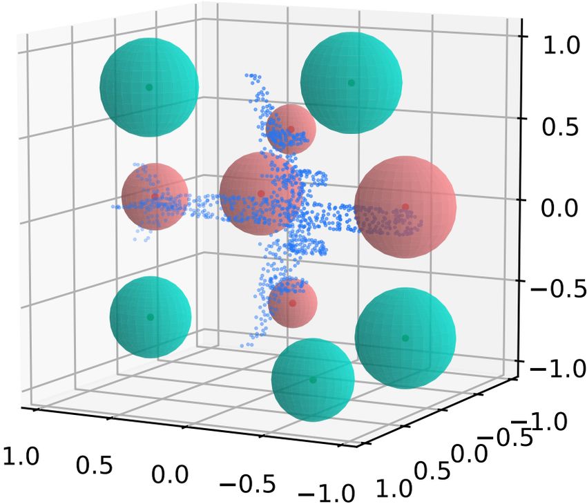
Figure 4: Accuracy curve with the corruption of (a) kernel number and (b) number of input points. (c)
and (d) visualize the kernel configurations when 5 and 300 kernels are used respectively. Each kernel
is displayed as a sphere, whose origin and radius decode the kernel center and size respectively.
-25% -50% -75% 0.05 0.1
PointNet 86.1 83.2 74.0 79.1 30.0
PointNet++ 89.5 87.9 86.5 82.3 45.1
ours(val.) 88.9 88.5 86.9 85.2 62.4
ours(enh.) 89.9 89.2 87.9 86.3 65.6
Table 3: Comparisons of classification accuracy on ModelNet 40. Left 3 columns: results with
random point dropout; right 2 columns: results with different Gaussian noise std..
Robustness to Noise and Incomplete Data. In the real-world capturing scenarios, the data ob-
tained from sensors is prone to be noisy and highly irregular. To validate the robustness of our
network to the non-uniform and sparse data, we train our network using 1024 points and test it
with random point dropout. Starting from 1024 points, we gradually decrease the amount of input
points. As shown in Figure 4b, when half of the points (512) are missing, the accuracy of both the
vanilla and enhanced network only drop by less than 1%. Our network can achieve more than 85%
accuracy when only 128 points are used: vanilla network - 85.3%; enhanced model - 87.8%. Our
approach is scalable to extremely sparse points. In particular, when only 32 input points are presented,
our enhanced network can still achieve 75.3% accuracy while the vanilla model reaches to 63.5%
accuracy.
We also compare the performance of our network with PointNet and PointNet++ when missing points
and noises are present (see Table 3). In the left part of Table 3 (left 3 columns), we compare the
classification accuracy in terms of varying degrees of random point dropout. The results demonstrate
that our approaches are much more robust than PointNet based networks especially when the
input point cloud becomes sparser. In the right two columns of Table 3, We compare the results
when Gaussian noise is added to each point independently. In particular, we test the candidate
approaches with the standard variation of Gaussian noises being 0.05 and 0.1 respectively. Our
solution significantly outperforms the PointNet structures. As shown in Table 3, our vanilla network
outperforms PointNet++ by more than 17% when the input point cloud is highly noisy (standard
deviation equals to 0.1).
Robustness to Kernel Density. As the nonlinear RBF kernels employed in our framework only
have localized response to the input points, one of our major concerns is whether the network scales
well to a sparse set of kernels. We test our approach with number of kernels ranging from 1 to 1000
as demonstrated in Figure 4a. To our surprise, the network works quite well even with two RBF
kernels - the vanilla and enhanced structure have achieved 76.7% and 84.8% accuracy respectively.
With five kernels, both networks have obtained accuracy higher than 84%: vanilla - 84.3%; enhanced
- 88.1%. When the number of kernels is further increased, the classification accuracy grows slowly
and achieves its maximum value at around 300. We visualize the optimized kernel distribution when
5 and 300 kernels are used for feature extraction in Figure 4c and Figure 4d respectively. As indicated
in the visualization, our method automatically increases the receptive field of kernels when kernel
density is small, enabling a faithful capture of the spatial point distribution even when extremely
sparse kernels are employed.
7Gs. Mk. IMQ Gs.+Mk. Gs.+IMQ
Vanilla 89.1 89.0 85.6 89.5 88.3
Enhan. 90.2 90.1 89.8 90.5 90.3
Table 4: Instance classification accuracy using various kernel functions and their combinations. "Gs."
stands for Gaussian while "Mk." stands for Markov.
Fix Center Fix Size Fix Both Optim. Both
Vanilla 88.6 75.2 72.9 89.1
Enhan. 89.5 87.5 86.8 90.2
Table 5: Effect of optimizing center position and receptive fields of kernels. Instance classification
accuracy (in percentage) is shown in the table.
Variations of Kernel Functions Our framework scales well to different types of kernel functions.
We investigate the performance of our algorithm by using three major types of RBF kernels: Gaussian,
Markov and Inverse Multiquadratic (IMQ). The three candidate kernel functions all have localized
activation but differ in the degrees of locality. In general, Gaussian kernel has the strongest localized
response, followed by the Markov function and the IMQ kernel. As demonstrated in Table 4, Gaussian
kernel has achieved the best classification accuracy in both versions of networks. The performance of
Markov function is comparable to that of Gaussian while the accuracy of IMQ is significantly lower
than the other two with the vanilla network. This suggests that more localized/nonlinear response
has stronger capability to extract more discriminative features. The enhanced structure, however,
has achieved high accuracy with all the three kernels. The additional MLP layer has boosted the
communication between the kernels, generating more effective features while providing stronger
robustness to the variations of learnt features.
Our approach is flexible to consider different kernels. In particular, similar to considering additional
input attributes , multiple channels of RBF layers are employed in which each channel employs a
unique kernel. The feature maps obtained from different channels are concatenated after the RBF
layer for further processing. As indicated in Table 4, it is interesting to observe that the mixture of
Gaussian and the other two kernels can produce even higher accuracy than applying them alone.
Importance of Optimizing Kernel Center and Nonlinearity. The center position and kernel size
are the two important parameters that completely determine the configuration of RBF layer. We
investigate the importance of each parameter by selectively fixing one of the components. Table 5
demonstrates the instance classification accuracy of four combinatorial settings. All the settings share
the same kernel initialization. As seen from the Table 5, optimizing both parameters have led to the
best performance while fixing both generates the worst results. If only optimizing kernel size (fixing
kernel centers), the accuracy of both networks only drop by less than one percent. However, in the
case of fixing the kernel sizes, the performance of both networks degrades significantly, especially
the vanilla structure. The experimental results indicate that an optimized nonlinearity of the RBF
kernels is the key to extracting discriminative features. As the initial kernel centers are randomly
dispersed inside the unit sphere, the kernels have been able to cover features from each local regions
via adjusting its receptive field. Hence, the optimization of kernel centers has less impact on the final
classification accuracy.
Robustness to Initial Kernel Distribution. As the capability to capture the spatial point distribu-
tion is the key to analyzing point clouds, we further validate the robustness of our algorithm to various
initial kernel distributions. We investigate five different scenarios: uniform distribution, random
sampling within a unit sphere, K-means clustering, overlapping kernels (all kernels are placed in
(0, 0, 0)) and random sampling from a local region. Figure 5 shows the kernel distribution before
and after optimization using the vanilla network. As seen from the results, our network strives
to scatter the initial points so as to capture features in a larger scale, especially when the initial
sampling is too crowded (see Figure 5d and Figure 5i). Hence our network is still capable to maintain
high classification accuracy when the initialization is strongly biased (88.7% for kernel overlapping;
8(a) (b) (c) (d) (e)
(f) Uniform (g) Random (h) K-means (i) Overlap (j) Local
Figure 5: Visualization of kernel distributions before (first row) and after (second row) optimization.
89.2% for localized initialization). As seen from Table 6, our approach is robust to different patterns
of initialization as long as kernels are dispersed in a global scale.
Uniform Rand. K-means Overlap Local
Vanilla 89.2 89.1 89.0 86.3 88.2
Enhan. 90.3 90.2 90.2 88.7 89.2
Table 6: Instance classification accuracy given different initial kernel initializations.
5 Conclusion
In this paper, we present deep RBFNet - a novel deep learning framework that utilizes nonlinear
mapping provided by RBF kernels for efficient learning of point cloud features. Unlike prior works
that obtain point features in an implicit manner, we explicitly model the spatial distribution of point
cloud by leveraging the localized nonlinearity of RBF kernels. The local receptive field of RBF kernels
enables discriminative patterns of activated kernels for different point distributions. Thanks to the
effective feature extraction, our approach has achieved comparable or even better performance in the
task of point cloud recognition comparing to the state-of-the-art methods. Furthermore, our algorithm
has reduced the number of network parameters by a considerable amount, enabling a remarkably
faster training than existing works. We also provide intuitive analysis towards understanding of our
networks.
References
[1] R Qi Charles, Hao Su, Mo Kaichun, and Leonidas J Guibas. Pointnet: Deep learning on
point sets for 3d classification and segmentation. In Computer Vision and Pattern Recognition
(CVPR), 2017 IEEE Conference on, pages 77–85. IEEE, 2017.
[2] Charles Ruizhongtai Qi, Li Yi, Hao Su, and Leonidas J Guibas. Pointnet++: Deep hierarchical
feature learning on point sets in a metric space. In Advances in Neural Information Processing
Systems, pages 5105–5114, 2017.
[3] Jonathan C Carr, Richard K Beatson, Jon B Cherrie, Tim J Mitchell, W Richard Fright, Bruce C
McCallum, and Tim R Evans. Reconstruction and representation of 3d objects with radial basis
functions. In Proceedings of the 28th annual conference on Computer graphics and interactive
techniques, pages 67–76. ACM, 2001.
[4] Robert Osada, Thomas Funkhouser, Bernard Chazelle, and David Dobkin. Shape distributions.
ACM Transactions on Graphics (TOG), 21(4):807–832, 2002.
9[5] A Ben Hamza and Hamid Krim. Geodesic object representation and recognition. In International
conference on discrete geometry for computer imagery, pages 378–387. Springer, 2003.
[6] Haibin Ling and David W Jacobs. Shape classification using the inner-distance. IEEE transac-
tions on pattern analysis and machine intelligence, 29(2):286–299, 2007.
[7] David S Broomhead and David Lowe. Radial basis functions, multi-variable functional interpo-
lation and adaptive networks. Technical report, Royal Signals and Radar Establishment Malvern
(United Kingdom), 1988.
[8] Mark JL Orr et al. Introduction to radial basis function networks, 1996.
[9] Gholam ali Montazer, Davar Giveki, Maryam Karami, and Homayon Rastegar. Radial basis
function neural networks: A review. Computer Reviews Journal, 1(1):52–74, 2018.
[10] Meng Joo Er, Shiqian Wu, Juwei Lu, and Hock Lye Toh. Face recognition with radial basis
function (rbf) neural networks. IEEE transactions on neural networks, 13(3):697–710, 2002.
[11] Yue Wu, Hui Wang, Biaobiao Zhang, and K-L Du. Using radial basis function networks for
function approximation and classification. ISRN Applied Mathematics, 2012, 2012.
[12] Roger D Jones, YC Lee, CW Barnes, GW Flake, K Lee, PS Lewis, and S Qian. Function
approximation and time series prediction with neural networks. In Neural Networks, 1990.,
1990 IJCNN International Joint Conference on, pages 649–665. IEEE, 1990.
[13] Zhirong Wu, Shuran Song, Aditya Khosla, Fisher Yu, Linguang Zhang, Xiaoou Tang, and
Jianxiong Xiao. 3d shapenets: A deep representation for volumetric shapes. In Proceedings of
the IEEE conference on computer vision and pattern recognition, pages 1912–1920, 2015.
[14] Daniel Maturana and Sebastian Scherer. Voxnet: A 3d convolutional neural network for real-
time object recognition. In Intelligent Robots and Systems (IROS), 2015 IEEE/RSJ International
Conference on, pages 922–928. IEEE, 2015.
[15] Yangyan Li, Soeren Pirk, Hao Su, Charles R Qi, and Leonidas J Guibas. Fpnn: Field probing
neural networks for 3d data. In Advances in Neural Information Processing Systems, pages
307–315, 2016.
[16] Hang Su, Subhransu Maji, Evangelos Kalogerakis, and Erik Learned-Miller. Multi-view convo-
lutional neural networks for 3d shape recognition. In Proceedings of the IEEE international
conference on computer vision, pages 945–953, 2015.
[17] Charles R Qi, Hao Su, Matthias Nießner, Angela Dai, Mengyuan Yan, and Leonidas J Guibas.
Volumetric and multi-view cnns for object classification on 3d data. In Proceedings of the IEEE
conference on computer vision and pattern recognition, pages 5648–5656, 2016.
[18] Peng-Shuai Wang, Yang Liu, Yu-Xiao Guo, Chun-Yu Sun, and Xin Tong. O-cnn: Octree-based
convolutional neural networks for 3d shape analysis. ACM Transactions on Graphics (TOG),
36(4):72, 2017.
[19] Gernot Riegler, Ali Osman Ulusoy, and Andreas Geiger. Octnet: Learning deep 3d represen-
tations at high resolutions. In Proceedings of the IEEE Conference on Computer Vision and
Pattern Recognition, volume 3, 2017.
[20] Roman Klokov and Victor Lempitsky. Escape from cells: Deep kd-networks for the recognition
of 3d point cloud models. In 2017 IEEE International Conference on Computer Vision (ICCV),
pages 863–872. IEEE, 2017.
[21] Tong He, Haibin Huang, Li Yi, Yuqian Zhou, Chihao Wu, Jue Wang, and Stefano Soatto.
Geonet: Deep geodesic networks for point cloud analysis. arXiv preprint arXiv:1901.00680,
2019.
[22] Yann LeCun, Léon Bottou, Yoshua Bengio, and Patrick Haffner. Gradient-based learning
applied to document recognition. Proceedings of the IEEE, 86(11):2278–2324, 1998.
10[23] Martín Abadi, Ashish Agarwal, Paul Barham, Eugene Brevdo, Zhifeng Chen, Craig Citro,
Greg S Corrado, Andy Davis, Jeffrey Dean, Matthieu Devin, et al. Tensorflow: Large-scale
machine learning on heterogeneous distributed systems. arXiv preprint arXiv:1603.04467,
2016.
[24] Diederik P Kingma and Jimmy Ba. Adam: A method for stochastic optimization. arXiv preprint
arXiv:1412.6980, 2014.
[25] Martin Simonovsky and Nikos Komodakis. Dynamic edge-conditioned filters in convolutional
neural networks on graphs. In Proc. CVPR, 2017.
[26] Manzil Zaheer, Satwik Kottur, Siamak Ravanbakhsh, Barnabas Poczos, Ruslan R Salakhutdinov,
and Alexander J Smola. Deep sets. In Advances in Neural Information Processing Systems,
pages 3394–3404, 2017.
11You can also read