Using hyperspectral imagery to investigate large scale seagrass cover and genus distribution in a temperate coast
←
→
Page content transcription
If your browser does not render page correctly, please read the page content below
www.nature.com/scientificreports
OPEN Using hyperspectral imagery
to investigate large‑scale seagrass
cover and genus distribution
in a temperate coast
Kenneth Clarke1, Andrew Hennessy1, Andrew McGrath2, Robert Daly3, Sam Gaylard4,
Alison Turner5, James Cameron5, Megan Lewis1 & Milena B. Fernandes 3,6*
Seagrasses are regarded as indicators and first line of impact for anthropogenic activities affecting the
coasts. The underlying mechanisms driving seagrass cover however have been mostly studied on small
scales, making it difficult to establish the connection to seagrass dynamics in an impacted seascape.
In this study, hyperspectral airborne imagery, trained from field surveys, was used to investigate
broadscale seagrass cover and genus distribution along the coast of Adelaide, South Australia. Overall
mapping accuracy was high for both seagrass cover (98%, Kappa = 0.93), and genus level classification
(85%, Kappa = 0.76). Spectral separability allowed confident genus mapping in waters up to 10 m
depth, revealing a 3.5 ratio between the cover of the dominant Posidonia and Amphibolis. The work
identified the absence of Amphibolis in areas historically affected by anthropogenic discharges, which
occasionally contained Posidonia and might be recovering. The results suggest hyperspectral imagery
as a useful tool to investigate the interplay between seagrass cover and genus distribution at large
spatial scales.
Seagrass meadows are hotspots for marine biodiversity, providing ecological functions that encompass biologi-
cal, geochemical and physical needs of marine life1. As a transition zone to the open ocean, seagrasses further
provide a variety of ecosystem services to humans. These include among others opportunities for recreation,
protection from erosion and sea level rise, carbon sequestration, offsetting of ocean acidification, and breeding
and nursery habitat for economically important species2–4. These functions and services are however threatened
by the high sensitivity of seagrasses to water q uality5, exacerbated by their generally high level of connectivity
with neighboring h abitats6. Successful management of these systems thus is intrinsically linked to a broader
understanding of the dynamics of meadows at the scale of the seascape (100 s m 2 to 1000 s of km2)7.
Remote sensing approaches provide an opportunity to inform management through integration of data at
meaningful spatial scales, but mapping of subtidal seagrasses is hindered by many factors including water reflec-
tion, scattering and absorption of light8. Despite these limitations, aerial photography and satellite imagery have
been used extensively to map change in seagrass meadows during the last century. Large worldwide losses have
been documented as a result of urbanization and land-use change9, while the curbing of anthropogenic pressures
has more recently seen a resurgence in regions as diverse as Chesapeake Bay, Southwest Florida estuaries, the
Baltic Sea, Atlantic coasts of Europe, and the Mediterranean S ea10–13. A combination of ecological and remote
sensing research indicates that complex mechanisms are associated with seagrass recovery, from small scale
dispersal to large scale connectivity, patch recruitment, rhizome elongation and patch coalescence, of individual
or multiple species7.
While at a broad geographical scale physical and chemical drivers define the dominant climax species in the
recovery sequence, time since disruption and species succession play a critical role in determining which species
are present at particular s tages14. As seagrasses are lost, denuded areas become more energetic and early recruit-
ment favours species with higher resistance to waves and currents, combined with high reproductive output15.
1
School of Biological Sciences, The University of Adelaide, Adelaide, SA 5005, Australia. 2Airborne
Research Australia, PO Box 335, Salisbury South, SA 5106, Australia. 3SA Water, GPO Box 1751, Adelaide,
SA 5001, Australia. 4South Australian Environment Protection Authority, GPO Box 2607, Adelaide,
SA 5001, Australia. 5Department for Environment and Water, GPO Box 1047, Adelaide, SA 5001,
Australia. 6College of Science and Engineering, Flinders University, GPO Box 2100, Adelaide, SA 5001,
Australia. *email: milena.fernandes@sawater.com.au
Scientific Reports | (2021) 11:4182 | https://doi.org/10.1038/s41598-021-83728-6 1
Vol.:(0123456789)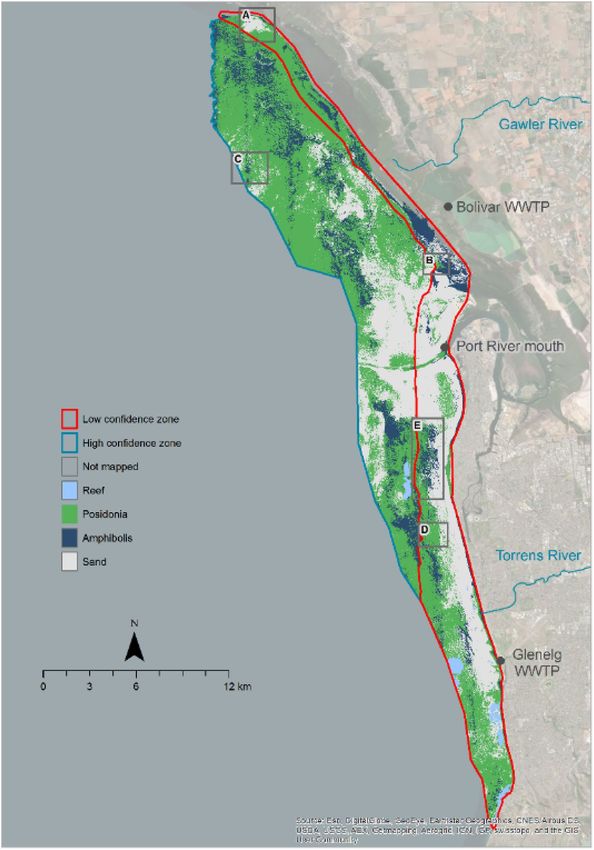
www.nature.com/scientificreports/
Reference (field) data
Mapped cover Seagrass Sand Total User’s accuracy (%)
Seagrass 30 1 31 97
Sand 0 9 9 100
Total 30 10 40
Producer’s accuracy (%) 100 90
Overall accuracy (%) 98
Table 1. Confusion matrix based on number of sites, and accuracy for the benthic cover classification.
These early colonisers act as ecosystem engineers and modify local conditions, allowing the establishment of
other species, which in time come to dominate the system. The susceptibility of individual species to external
drivers is thus an important determinant in the successional sequence and overall recovery t ime16. Changes in
seagrass cover however are usually mapped as seagrass presence or absence, with less information available to
determine mechanisms of change, such as the interplay between species, or the progression of cover density
(e.g. from sparse to dense). Progress in remote sensing technology has provided a pathway to investigate these
knowledge gaps, particularly through increased spatial and spectral resolution associated with the development
of multispectral and hyperspectral s ensors17.
In this study we used airborne hyperspectral imagery to investigate seagrass cover and genus distribution in
a coastal metropolitan region (Adelaide, South Australia) dominated by Posidonia and Amphibolis, two temper-
ate seagrass genera with distinct life history traits. Posidonia is considered a persistent genus highly resistant to
disturbance18. Once lost, recovery is compromised by comparatively low and unreliable seed production and
slow rhizome growth, among other factors. Amphibolis in contrast is considered an opportunistic genus, with
the ability to release seedlings that can rapidly colonise areas where seagrass loss resulted in increased hydro-
dynamic forcing19. As the seeds of Posidonia lack dormancy and Amphibolis relies on the dispersal of seedlings,
recovery is dependent on short windows of opportunity for the successful establishment of new r ecruits20. This
study investigated the benefits and limitations of the use of airborne hyperspectral imagery to differentiate these
seagrass genera in the seascape, and map overall seagrass cover. The data was then interpreted in terms of natural
or anthropogenic drivers driving seagrass spatial dynamics.
Results
The overall accuracy of benthic cover mapping was 98%, with only one sand site mapped as seagrass (Table 1).
Although this accuracy assessment was based on a relatively small number of sites, a high Cohen’s kappa coef-
ficient of 0.93 confirmed very strong agreement between field data and mapped cover. The classification revealed
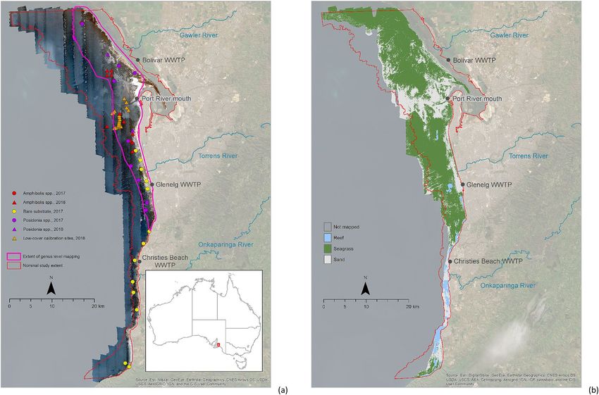
42,298 ha of seagrass (70% of the study area) and 18,395 ha of sand (Fig. 1b). Sand was mostly prevalent in the
vicinity of the Port River shipping channel, and in the first 1–2 km from shore north and south of the Torrens
River. Visual fragmentation of seagrass cover also occurred further offshore south of the Torrens River and off
the Gawler River.
The analysis of genus spectral separability was performed on the highest quality portions of the imagery
through the visual selection of reference sites, thus establishing separability under near ideal conditions. Jeffries-
Matusita (J-M) distance followed an approximately linear decline with water depth, starting with perfect separa-
bility at 1–2 m and decreasing to a minimum at 9 m (Fig. 2). True separability probably continues to decline with
depth, but an artefactual increase was calculated from 9 to 11 m due to the difficulty in locating reference sites in
this depth range. The genus level classification was thus limited to 10 m water depth. The smaller area mapped
to genus level (29,196 ha) in comparison to total benthic cover (60,693 ha) (Fig. 1a) highlights this sensitivity of
the genus classification to water depth.
Spectral differences between genera were further compromised by slight sensor saturation nearshore, leading
to a ‘low confidence zone’ in classification (Fig. 3). In this zone, original spatial patterns (e.g. annotation B in
Fig. 3) and visibly discernible differences between classes (e.g. annotation D) were sometimes lost. The addition
of a depth variable tended to degrade classification, while the inclusion of latitude and longitude improved class
discrimination, particularly in deeper regions where it prevented over-classification of Amphibolis. Other chal-
lenges encountered in the genus classification included the presence of suspended sediment nearshore leading
to sand over-classification (annotation A), and variation of image quality between adjoining flight lines resulting
in unsightly abrupt changes in classification (e.g. annotation C).
Despite limitations, overall accuracy of the genus classification was high at 85%, ranging from 80% in the low
confidence zone to 93% in the high confidence zone, with only a few Amphibolis sites classified as Posidonia, and
one sand site classified as Amphibolis (Table 2). The Cohen’s kappa coefficient of 0.76 further confirmed strong
agreement between field and mapped cover, varying between 0.69 in the low confidence zone to 0.86 in the high
confidence zone. The classification indicated dominance of Posidonia (53%) over sand (32%) or Amphibolis (15%)
(Fig. 3). Amphibolis was more prevalent at the landward edge of the seagrass distribution and at mid-depths
(~ 3–7 m in the north and 5–9 m in the south), but largely disappeared in a 5 km radius from the Port River
mouth, and off the Gawler and Torrens rivers.
Scientific Reports | (2021) 11:4182 | https://doi.org/10.1038/s41598-021-83728-6 2
Vol:.(1234567890)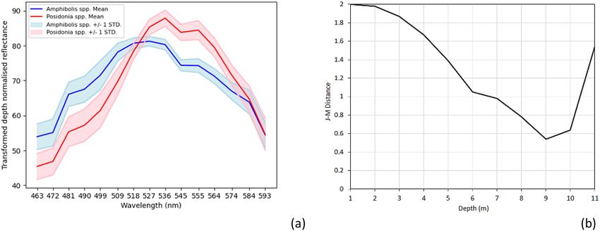
www.nature.com/scientificreports/
Figure 1. Sunglint corrected, pseudo true-colour image composite of the 2018 hyperspectral imagery (a), and
benthic cover classification of this imagery (b). On the left panel, the nominal study area is outlined in red, and
the extent of genus classification (Fig. 3) in purple. Field locations of large patches of homogeneous Amphibolis,
Posidonia and sand cover used for accuracy assessment are differentiated by year of record (circle = 2017,
triangle = 2018). Location of sites further investigated in 2018 to clarify suspected low cover are also presented.
Map created in ESRI ArcGIS 10.7; terrestrial ESRI Basemap World Imagery (https://www.esri.com/en-us/arcgis/
products/arcgis-enterprise).
Figure 2. Mean spectral signature of Amphibolis and Posidonia in shallow (1–2 m) waters (a), and spectral
separability indicated by Jeffries-Matusita (J-M) distance with water depth (b).
Scientific Reports | (2021) 11:4182 | https://doi.org/10.1038/s41598-021-83728-6 3
Vol.:(0123456789)www.nature.com/scientificreports/
Figure 3. Seagrass genus classification in 2018, with annotations A–E highlighting areas discussed in the text.
Map created in ESRI ArcGIS 10.7; terrestrial ESRI Basemap World Imagery (https://www.esri.com/en-us/arcgis/
products/arcgis-enterprise).
Scientific Reports | (2021) 11:4182 | https://doi.org/10.1038/s41598-021-83728-6 4
Vol:.(1234567890)www.nature.com/scientificreports/
Reference (field) data
Mapped cover Amphibolis Posidonia Sand Total User’s accuracy (%)
Study area
Amphibolis 10 0 1 11 91
Posidonia 4 14 0 18 78
Sand 0 0 5 5 100
Total 14 14 6 34
Producer’s accuracy (%) 71 100 83
Overall accuracy (%) 85
High confidence zone
Amphibolis 7 0 0 7 100
Posidonia 1 6 0 7 86
Sand 0 0 0 0 N/A
Total 8 6 0 14
Producer’s accuracy (%) 87 100 N/A
Overall accuracy (%) 93
Low confidence zone
Amphibolis 3 0 1 4 75
Posidonia 3 8 0 11 73
Sand 0 0 5 5 100
Total 6 8 6 20
Producer’s accuracy (%) 50 100 83
Overall accuracy (%) 80
Table 2. Confusion matrix based on number of sites, and accuracy for the genus level classification.
Discussion
The study presented here is arguably the most successful mapping of benthic exposure for the Adelaide metro-
politan coastline, covering a larger extent than previous s tudies21–24, and with high accuracy. The benthic cover
mapping (sand vs seagrass) had very high accuracy (98% overall accuracy, Kappa = 0.93), and the genus classifi-
cation had high accuracy (85% overall accuracy, Kappa = 0.76). These accuracies compare favourably with other
similar studies, typically ranging between 50 and 75%17,25. The mapping success is explained by the high spectral
resolution of the sensor in the range where water transparency is highest, combined with its high signal to noise
and high dynamic range, further improved by pre-processing to remove s unglint26 and normalize illumination
with depth25. Mapped seagrass cover however was conservative for both mapping products (benthic cover and
genus) because the image spatial resolution (2 m) and classification based on similarity to either sand or dense
seagrass spectral signatures hinders the detection of cm-scale patches of early colonization if these patches are not
the dominant class in a pixel. The mapping approach needs further tuning to the specific mapping goal, requiring
slightly different solutions for the benthic cover and the genus mapping. For example, tuning image acquisition
for genus classification requires careful consideration of signal integration time to allow genus discrimination
in deeper waters while minimising sensor signal saturation in the nearshore.
The benthic cover mapping revealed extensive seagrass meadows covering 70% of the study area. The genus
classification suggests that Posidonia and Amphibolis distribution is intertwined, with Amphibolis preferentially
found at the landward edge of meadows and at mid-depths. The map of genus cover corroborates observations of
an Amphibolis province around Point Malcolm (annotation E, Fig. 3) recorded more than a decade earlier using
multispectral satellite imagery27, and video transects, as well as the historical reconstruction of records going
back to the 1 970s28, suggesting these are long-term features of the Adelaide coast rather than a point in time
in the successional sequence. Although Amphibolis is considered an early colonizer in highly dynamic regions
through the development of deep vertical roots and wiry stems29, it can also become the climax species in areas
with high rates of physical d isturbance15.
The spatial pattern of Amphibolis distribution was disrupted in the vicinity of the Port River shipping chan-
nel, off the Gawler River, and nearshore north and south of the Torrens River, areas where existing seagrass was
largely classified as Posidonia. Previous studies28,30 have raised selective loss as a mechanism to explain Amphibolis
absence in a number of locations along the Adelaide coast affected by historically large nutrients and suspended
solids inputs. The genus has a low tolerance to reduced light conditions, particularly when driven by epiphyte
cover31,32, and its recovery in disturbed systems is considered notoriously difficult, even when loss is driven by
factors other than water quality33. Posidonia instead was observed in some areas largely classified as bare sand
for the last 2–3 d ecades21–24,34, e.g. the western boundary offshore of the Amphibolis province off Point Malcolm,
and in the nearshore embayment south of the Port River mouth. Video transects (Fig. 1a) confirm the presence of
Posidonia but mixed with Zostera and occasionally sparse Halophila and Pinna bicolor (razorfish). This potential
recovering trend follows the decommissioning of sludge outfalls in 199334,35, the closure of a soda ash factory in
the Port River in 2 01336 and continuous improvement of wastewater d ischarges37,38.
Scientific Reports | (2021) 11:4182 | https://doi.org/10.1038/s41598-021-83728-6 5
Vol.:(0123456789)www.nature.com/scientificreports/
In conclusion, the use of hyperspectral imagery provides improved monitoring of seagrass dynamics at the
scale of the seascape, achieving high spatial resolution and accuracy in the mapping of both benthic cover as well
as genus distribution. Where inputs from land had been historically high, Amphibolis is absent, but Posidonia
is still recorded and is likely recovering following a reduction in discharges. The data from this study provides
a baseline from which our understanding of the responses of individual genera can be further refined in the
future with subsequent mapping. Future mapping should also consider the inclusion of genera which although
comparatively rare in the seascape (e.g. Zostera) might play a critical successional role.
Methods
Study area. The study area covered 784 k m2 in coastal waters up to 17 m depth off Adelaide, South Australia
(Fig. 1a). The climate is Mediterranean and rainfall occurs primarily in winter38. These oligotrophic waters sup-
port vast meadows of Posidonia sinuosa, Posidonia angustifolia and Amphibolis antarctica28. The physical setting
is determined by prevailing waves from the southwest, generated by wind and oceanic swell39. The chemical
setting is currently driven by discharges from three wastewater treatment plants and three rivers, all in close
proximity to each other38. These inputs affect the light climate through suspended solids and phytoplankton in
the water column, and epiphytes growing on seagrass leaves40. Seagrass loss was first recorded from the 1950s,
peaking in the 1970s21–24. The total area of loss was estimated at over 6,200 ha by the late 2000s19. The first signs
of recovery started to appear in 201324.
Field data. Nineteen sites were surveyed between March and May 2017 through the regular monitoring
program of the South Australian Environment Protection Authority (EPA). Sites were selected between 2 and
15 m water depth by random sampling design using a 500 × 500 m grid overlayed on bathymetry, with the
number of sites and replication within sites (transects) based on the power afforded by results from previous
surveys41. At each 20 ha site, 10 random 50 m video transects were surveyed. Transects were undertaken using
a geo-referenced 450-line analogue video camera (Scielex) angled at 90 degrees to the seafloor. A live video feed
to a surface screen viewed by a trained operator ran directly from the camera into an audio and video encoding
system (Geostamp) which overlays a GPS location, direction, speed, date and time strings to the video and on
a hard drive. The set-up of the camera provided a field of view of approximately 1 m 2, allowing post-processing
to classify seagrass cover as either low (< 50%), medium (50–75%) or dense (> 75%) over 1 m increments. Loca-
tions used for accuracy assessment of image classification (Fig. 1a) were the centre point of a transect segment
covering an area of homogenous dense cover at least 26 m long. Locations with smaller spatial extents of dense
cover were used for image interpretation or definition of training areas. Field data spatial uncertainty was con-
servatively estimated as 12 m based on GPS uncertainty (< 10 m), and variable distance of camera from GPS
(< 2 m). The EPA transects were complemented by field surveys in 2018 to locate additional areas for accuracy
assessment of image classification, and to calibrate the classification in areas of suspected low cover (< 50%) in
21 additional sites of 4 transects in the vicinity of the Port River shipping channel (Fig. 1a).
Airborne imagery. Airborne imagery was acquired in late summer (8–9 March 2018). A Diamond HK-36
ECO-Dimona aircraft was fitted with a hyperspectral linescanner (modified Specim AISA Eagle 2) acquiring 62
spectral bands of 9.5 nm from 408.5 to 990.6 nm. The raw data was recorded with GNSS time for the centre of
the integration period for each captured frame. The spatial resolution was 2 m, and integration time 25 ms, an
interval selected to just reach sensor saturation on land and maximise the ability to image deeper waters. North–
South flight lines were oriented as near as practical to the direction of the solar azimuth to minimize cross-track
bidirectional reflectance and sunglint. The image swath was approximately 1900 m, with 1 km spacing between
tracks to allow for overlap. Supporting instrumentation included an RT-4003 precision navigation unit (Oxford
Technical Solutions) incorporating a dual-GNSS system and IMU rigidly mounted with the hyperspectral sen-
sor.
Post-processing combined the raw aircraft GNSS and IMU data with data from a deployed NovAtel DL-V3
GNSS ground station as well as publicly available base stations and post-hoc precision satellite ephemeris data.
Accurate frame timing allowed correlation with post-processed navigation data to deliver location and 3-axis
orientation of the optical axis for each frame. Imagery spatial uncertainty was conservatively estimated as 8 m
based on IMU position and orientation performance, instrument optics and timing accuracy of the hyperspectral
frames over the integration time. Raw hyperspectral frames were processed to at-sensor radiances using a 2015
radiometric calibration, with five seconds of dark-frame data collected at the end of each flight line. ATCOR-4
software42 was used to derive at-surface reflectances, assuming a standard library maritime atmosphere with
70 km visibility.
Imagery classification. Image processing and map production was performed across Python, ENVI and
ArcGIS. Sunglint removal and depth normalisation algorithms were implemented in Python. Spectral subset-
ting, imagery classification, majority filtering, and J-M distance were all performed in ENVI 5.3. Maps were
produced in ArcGIS 10.7.
Benthic cover classification. Imagery pre-processing involved sunglint removal26 and spectral subsetting to
exclude bands with poor signal-to-noise ratio interpreted as substantial visible random variation in brightness
within cover types. Bands 7 (463.0 nm) through to 21 (593.6 nm), and band 62 (990.6 nm) were retained.
After pre-processing, training areas of 5 × 5 pixels were defined for each substrate class in each flight line until
approximately 2,000 pixels were selected based on visual interpretation and field data. Training areas of 5 × 5
pixels encompassed an area large enough (100 m2) to locate with confidence given spatial uncertainty (< 12 m),
Scientific Reports | (2021) 11:4182 | https://doi.org/10.1038/s41598-021-83728-6 6
Vol:.(1234567890)www.nature.com/scientificreports/
and using 2,000 pixels identified 80 distinct training areas, a number that represents a good balance between
optimising training time and selecting enough appropriate training areas in the available field data. The bare
substrate class is referred to as sand, and the non-substrate class as seagrass. Explicit distinction of macroalgae
was not possible due to the absence of known macroalgae areas for classification training, but macroalgae cover
is expected to be small. The location of reefs was supplied as shapefiles by the Department for Environment and
Water of South Australia.
A Mahalanobis distance supervised classification was applied to each flight line, and classified imagery mosai-
cked into a single map. In areas of overlap priority was given to higher quality imagery, i.e. where wave action
was lowest, or where turbidity was lowest, or where sunglint was minimal, or in areas of sunglint, where sunglint
removal was more successful. The Mahalanobis classifier was chosen as the most successful after testing several
classifiers. As training areas had medium to dense seagrass, pixels classified as seagrass are estimated to con-
tain > 50% seagrass cover. Majority filtering (10 × 10 m) was used to reduce occasional pixel misclassification
related to wave action, turbidity and sunglint. Terrestrial and intertidal areas were masked, as well as all areas
of low- or no-confidence due to water depth, cloud cover or shadow, or suspended sediment, as well as areas of
seagrass wrack and breaking waves on beaches.
Genus classification. Genus classification included spectral subsetting and sunglint removal as described above,
as well as illumination difference normalisation with d epth25. Training areas of 5 × 5 pixels were defined for each
substrate class in each flight line based on visual interpretation and field data until approximately 1500–3000
pixels were selected (more for flight lines with more within- and between-class variability). The image was clas-
sified into Amphibolis, Posidonia and sand, using Support Vector Machine (SVM) supervised classification with
linear function kernels. The SVM classifier was chosen as the most successful after testing several classifiers.
The effect of including depth and latitude/longitude variables in the supervised classification was also tested.
The mosaicking of classified flight lines into a single map of genus cover included majority filtering (10 × 10 m)
and masking. In addition, the spectral separability of Amphibolis and Posidonia with bathymetric depth was
calculated by J-M distance for training spectra recorded at field data locations, with 0 indicating no separability
and 2 complete separation. The bathymetry40 was derived from the Adelaide Coastal Waters Study39 in the Port
Adelaide and Barker Inlet area, and from the Australian bathymetry and topography g rid43 elsewhere. Reference
sites of approximately 5 × 5 pixels were selected for both seagrass genera from 1 to 11 m water depth, including
9386 Amphibolis pixels and 14,025 Posidonia pixels.
Accuracy assessment. The combined 2017/2018 field dataset allowed accuracy assessment of the sand (n = 10)
versus seagrass classification (n = 30), as well as accuracy assessment of the genus classification into Amphibo-
lis (n = 14), Posidonia (n = 14), and sand (n = 6). Standard spatial accuracy statistics were computed, including
Overall accuracy (% of reference sites mapped correctly), Producer’s accuracy (% of real features mapped cor-
rectly), and User’s accuracy (% of classes mapped correctly). The Cohen’s kappa coefficient was also calculated,
with a value of 0 suggesting chance agreement between field and mapped data, and 1 complete agreement.
Data availability
The datasets generated during the current study are available from Figshare on https://doi.org/10.25909/14752
005.
Received: 5 February 2020; Accepted: 29 January 2021
References
1. York, P. H., Hyndes, G. A., Bishop, M. J. & Barnes, R. S. Faunal assemblages of seagrass ecosystems. In Seagrasses of Australia. Struc-
ture, Ecology and Conservation (eds A. W. D. Larkum, G. A. Kendrick, & P. J. Ralph) Ch. 17, 541–588 (Springer, Berlin, 2018).
2. Nordlund, L. M., Koch, E. W., Barbier, E. B. & Creed, J. C. Seagrass ecosystem services and their variability across genera and
geographical regions. PLoS ONE 11, e0163091 (2016).
3. Camp, E. F. et al. Mangrove and seagrass beds provide different biogeochemical services for corals threatened by climate change.
Front. Mar. Sci. 3, 52 (2016).
4. Gaylard, S. G., Waycott, M. & Lavery, P. S. Review of coast and marine ecosystems in temperate Australia demonstrate a wealth of
ecosystem services. Front. Mar. Sci. 7, 453 (2020).
5. Burkholder, J. M., Tomasko, D. A. & Touchette, B. W. Seagrasses and eutrophication. J. Exp. Mar. Biol. Ecol. 350, 46–72 (2007).
6. Kendrick, G. A. et al. Demographic and genetic connectivity: the role and consequences of reproduction, dispersal and recruitment
in seagrasses. Biol. Rev. 92, 921–938 (2017).
7. Kendrick, G. A. et al. Australian seagrass seascapes: present understanding and future research directions. In Seagrasses of Australia.
Structure, Ecology and Conservation (eds Anthony W.D. Larkum, Gary A. Kendrick, & Peter J. Ralph) Ch. 9, 257–286 (Springer,
Berlin, 2018).
8. Hossain, M. S., Bujang, J. S., Zakaria, M. H. & Hashim, M. The application of remote sensing to seagrass ecosystems: an overview
and future research prospects. Int. J. Remote Sens. 36, 61–114 (2015).
9. Waycott, M. et al. Accelerating loss of seagrasses across the globe threatens coastal ecosystems. Proc. Natl. Acad. Sci. USA 106,
12377–12381 (2009).
10. Lefcheck, J. S. et al. Long-term nutrient reductions lead to the unprecedented recovery of a temperate coastal region. Proc. Natl.
Acad. Sci. USA 115, 3658–3662 (2018).
11. Tomasko, D. et al. Widespread recovery of seagrass coverage in Southwest Florida (USA): temporal and spatial trends and manage-
ment actions responsible for success. Mar. Pollut. Bull. 135, 1128–1137 (2018).
12. Carmen, B. et al. Recent trend reversal for declining European seagrass meadows. Nat. Commun. 10, 3356 (2019).
13. Reise, K. & Kohlus, J. Seagrass recovery in the northern Wadden Sea?. Helgol. Mar. Res. 62, 77 (2008).
14. Kendrick, G. A., Holmes, K. W. & Niel, K. P. V. Multi-scale spatial patterns of three seagrass species with different growth dynamics.
Ecography 31, 191–200 (2008).
Scientific Reports | (2021) 11:4182 | https://doi.org/10.1038/s41598-021-83728-6 7
Vol.:(0123456789)www.nature.com/scientificreports/
15. Kirkman, H. Community structure in seagrasses in southern Western Australia. Aquat. Bot. 21, 363–375 (1985).
16. Rasheed, M. A. Recovery and succession in a multi-species tropical seagrass meadow following experimental disturbance: the role
of sexual and asexual reproduction. J. Exp. Mar. Biol. Ecol. 310, 13–45 (2004).
17. Fearns, P. R. C., Klonowski, W., Babcock, R. C., England, P. & Phillips, J. Shallow water substrate mapping using hyperspectral
remote sensing. Cont. Shelf Res. 31, 1249–1259 (2011).
18. Kilminster, K. et al. Unravelling complexity in seagrass systems for management: Australia as a microcosm. Sci. Total Environ.
534, 97–109 (2015).
19. Tanner, J. E. et al. Seagrass rehabilitation off metropolitan Adelaide: a case study of loss, action, failure, and success. Ecol. Manage.
Restor. 15, 168–179 (2014).
20. Sherman, C. D. et al. Reproductive, dispersal and recruitment strategies in australian seagrasses. In Seagrasses of Australia. Struc-
ture, Ecology and Conservation (eds Anthony W.D. Larkum, Gary A. Kendrick, & Peter J. Ralph) Ch. 8, 213–256 (Springer, Berlin,
2018).
21. Hart, D. Near-shore seagrass change between 1949 and 1996 mapped using digital aerial orthophotography, metropolitan Adelaide
area, Largs Bay-Aldinga, South Australia. A report prepared for the South Australian EPA. 12 (Department of Environment and
Natural Resources, Adelaide, South Australia, 1997).
22. Cameron, J. Near-shore seagrass change between 1995/6 and 2002 mapped using digital aerial orthophotography, metropolitan
Adelaide area, North Haven-Sellicks Beach, South Australia. 21 (South Australian Department for Environment and Heritage,
Adelaide, South Australia, 2003).
23. Cameron, J. Near-shore seagrass change between 2002 and 2007 mapped using digital aerial orthophotography, metropolitan
Adelaide area, Port Gawler-Marino, South Australia. 27 (Environment Protection Authority and Department for Environment
and Heritage, Adelaide, South Australia, 2008).
24. Hart, D. Seagrass extent change 2007–13 - Adelaide coastal waters. DEWNR technical note 2013/07. 19 (Department of Environ-
ment Water and Natural Resources, Adelaide, South Australia, 2013).
25. Pu, R., Bell, S., Baggett, L., Meyer, C. & Zhao, Y. Discrimination of seagrass species and cover classes with in situ hyperspectral
data. J. Coast. Res. 28, 1330–1344 (2012).
26. Hedley, J. D., Harborne, A. R. & Mumby, P. J. Simple and robust removal of sun glint for mapping shallow-water benthos. Int. J.
Remote Sens. 26, 2107–2112 (2005).
27. Blackburn, D. T. & Dekker, A. G. Remote sensing study of marine and coastal features and interpretation of changes in relation
to natural and anthropogenic processes. Final Technical Report. ACWS Technical Report No.6 prepared for the Adelaide Coastal
Waters Study Steering Committee. 177 (David Blackburn Environmental Pty Ltd and CSIRO Land and Water, Adelaide, South
Australia, 2006).
28. Bryars, S. & Rowling, K. Benthic habitats of Eastern Gulf St Vincent: major changes in benthic cover and composition following
European settlement of Adelaide. Trans. R. Soc S. Aust. 133, 318–338 (2009).
29. Kuo, J., Cambridge, M. L. & Kirkman, H. Anatomy and structure of australian seagrasses. In Seagrasses of Australia. Structure,
Ecology and Conservation (eds Anthony W.D. Larkum, Gary A. Kendrick, & Peter J. Ralph) Ch. 4, 93–125 (Springer, Berlin, 2018).
30. Neverauskas, V. P. Monitoring seagrass beds around a sewage sludge outfall in South Australia. Mar. Pollut. Bull. 18, 158–164
(1987).
31. Bryars, S., Collings, G. & Miller, D. Nutrient exposure causes epiphytic changes and coincident declines in two temperate Austral-
ian seagrasses. Mar. Ecol. Prog. Ser. 441, 89–103 (2011).
32. Neverauskas, V. P. Accumulation of periphyton biomass on artificial substrates deployed near a sewage sludge outfall in South
Australia. Est. Coast. Shelf Sci. 25, 509–517 (1987).
33. Burnell, O. W., Connell, S. D., Irving, A. D. & Russell, B. D. Asymmetric patterns of recovery in two habitat forming seagrass spe-
cies following simulated overgrazing by urchins. J. Exp. Mar. Biol. Ecol. 448, 114–120 (2013).
34. Westphalen, G. et al. A review of seagrass loss on the Adelaide metropolitan coastline. Adelaide Coastal Waters Study Technical
Report No. 2, August 2004. SARDI Aquatic Sciences Publication No. RD04/0073. 68 (South Australian Research & Development
Institute, Adelaide, South Australia, 2004).
35. Bryars, S. & Neverauskas, V. Natural recolonisation of seagrasses at a disused sewage sludge outfall. Aquat. Bot. 80, 283–289 (2004).
36. McDowell, L.-M. & Pfennig, P. Adelaide Coastal Water Quality Improvement Plan (ACWQIP) 162 (Adelaide, South Australia, 2013).
37. Cheshire, A. C. Adelaide Coastal Waters fore-sighting workshop report. Prepared for SA Environment Protection Authority. 102
(Science to Manage Uncertainty, Adelaide, South Australia, 2018).
38. Wilkinson, J. et al. Volumes of inputs, their concentrations and loads received by Adelaide metropolitan coastal waters. ACWS
Technical Report No. 18 prepared for the Adelaide Coastal Waters Study Steering Committee. 83 (Flinders Centre for Coastal and
Catchment Environments (Flinders University of SA), Adelaide, South Australia, 2005).
39. Pattiaratchi, C., Newgard, J. & Hollings, B. Physical oceanographic studies of Adelaide coastal waters using high resolution model-
ling, in-situ observations and satellite techniques – Sub Task 2 Final Technical Report. ACWS Technical Report No. 20 prepared
for the Adelaide Coastal Waters Study Steering Committee. 92 (School of Environmental Systems Engineering (The University of
Western Australia), Crawley, Australia, 2007).
40. van Gils, J., Erftemeijer, P. L. A., Fernandes, M. & Daly, R. Development of the Adelaide Receiving Environment Model. Deltares
report 1210877–000. 152 (Delft, the Netherlands, 2017).
41. Gaylard, S., Nelson, M. & Noble, W. The South Australian monitoring, evaluation and reporting program for aquatic ecosystems:
Rationale and methods for the assessment of nearshore marine waters. 70 (Environment Protection Authority, Adelaide, South
Australia, 2013).
42. Richter, R. & Schläpfer, D. Atmospheric/Topographic Correction for Airborne Imagery, ATCOR-4 User Guide, Version 4.2. 125
(DLR, Wessling, Germany, 2007).
43. Whiteway, T. Australian Bathymetry and Topography Grid. Record 2009/21. (Geoscience Australia, Canberra, 2009).
Acknowledgements
This project was funded by the South Australian Water Corporation (SA Water), the South Australian Environ-
ment Protection Authority (EPA) and the Department for Environment and Water (DEW). We are grateful to
M. Royal (DEW) for advice on study design, to W. Noble (EPA) for sharing and advising on field datasets, to
Tim Kildea (SA Water) for assistance with the collection of additional field data, and to the seabed rods program
team of the Coast and Marine Branch (DEW) for data and advice on genus distribution.
Author contributions
M.B.F. and K.C. led the writing of the original draft, M.B.F., J.C. and S.G. conceived the research, A.Mc.G.
designed airborne surveys, collected and processed imagery, K.C., A.H. and M.L. developed the methodol-
ogy for, and performed the benthic classifications, including accuracy assessment, S.G. provided field benthic
habitat data, R.D. collected and analysed additional field data, and provided GIS expertise, A.T. helped in the
Scientific Reports | (2021) 11:4182 | https://doi.org/10.1038/s41598-021-83728-6 8
Vol:.(1234567890)www.nature.com/scientificreports/
interpretation of genus distribution based on data from DEW’s long-term seabed rods program dive transects,
all authors contributed critically to the drafts and gave final approval for publication.
Competing interests
The authors declare no competing interests.
Additional information
Correspondence and requests for materials should be addressed to M.B.F.
Reprints and permissions information is available at www.nature.com/reprints.
Publisher’s note Springer Nature remains neutral with regard to jurisdictional claims in published maps and
institutional affiliations.
Open Access This article is licensed under a Creative Commons Attribution 4.0 International
License, which permits use, sharing, adaptation, distribution and reproduction in any medium or
format, as long as you give appropriate credit to the original author(s) and the source, provide a link to the
Creative Commons licence, and indicate if changes were made. The images or other third party material in this
article are included in the article’s Creative Commons licence, unless indicated otherwise in a credit line to the
material. If material is not included in the article’s Creative Commons licence and your intended use is not
permitted by statutory regulation or exceeds the permitted use, you will need to obtain permission directly from
the copyright holder. To view a copy of this licence, visit http://creativecommons.org/licenses/by/4.0/.
© The Author(s) 2021, corrected publication 2021
Scientific Reports | (2021) 11:4182 | https://doi.org/10.1038/s41598-021-83728-6 9
Vol.:(0123456789)You can also read