ERIC: Extracting Relations Inferred from Convolutions
←
→
Page content transcription
If your browser does not render page correctly, please read the page content below
ERIC: Extracting Relations Inferred from
                                                             Convolutions

                                                            Joe Townsend1[0000−0002−5478−0028] , Theodoros
                                                         1[0000−0003−2008−5817]
                                             Kasioumis                      , and Hiroya Inakoshi1[0000−0003−4405−8952]

                                             Fujitsu Laboratories of Europe LTD, 4th Floor, Building 3, Hyde Park Hayes, 11
arXiv:2010.09452v1 [cs.LG] 19 Oct 2020

                                                      Millington Road, Hayes, Middlesex, UB3 4AZ, United Kingdom
                                              {joseph.townsend,theodoros.kasioumis,hiroya.inakoshi}@uk.fujitsu.com

                                                 Abstract. Our main contribution is to show that the behaviour of ker-
                                                 nels across multiple layers of a convolutional neural network can be ap-
                                                 proximated using a logic program. The extracted logic programs yield
                                                 accuracies that correlate with those of the original model, though with
                                                 some information loss in particular as approximations of multiple layers
                                                 are chained together or as lower layers are quantised. We also show that
                                                 an extracted program can be used as a framework for further under-
                                                 standing the behaviour of CNNs. Specifically, it can be used to identify
                                                 key kernels worthy of deeper inspection and also identify relationships
                                                 with other kernels in the form of the logical rules. Finally, we make
                                                 a preliminary, qualitative assessment of rules we extract from the last
                                                 convolutional layer and show that kernels identified are symbolic in that
                                                 they react strongly to sets of similar images that effectively divide output
                                                 classes into sub-classes with distinct characteristics.

                                         1     Introduction
                                         As public concern regarding the extent to which artificial intelligence can be
                                         trusted increases, so does the demand for so-called explainable AI. While ac-
                                         countability is a key motivator in recent years, other motivations include un-
                                         derstanding how models may be improved, knowledge discovery through the
                                         extraction of concepts learned by the models but previously unknown to domain
                                         experts, means by which to test models of human cognition, and perhaps others.
                                             This has led to extensive research into explaining how models trained through
                                         machine learning make their decisions [1,2,3], and the field of Neural-Symbolic In-
                                         tegration covers this work with respect to neural networks [4,5,6,7,8]. The latter
                                         began by largely focussing on modelling the behaviour of multi-layer perceptrons
                                         or recurrent neural networks as symbolic rules that describe strongly-weighted
                                         relationships between neurons in adjacent layers [4,5]. More recent work strives
                                         to explain deeper networks, including convolutional neural networks (CNNs)
                                         [5,7,6,8]. Most of these methods identify important input or hidden features
                                         with respect to a given class or convolutional kernel [9,10,11,12,13,14,15], but
                                         methods that extract rule or graph-based relationships between key features are
                                         also emerging [16,17,18,19,20,21]. Moreover it has been shown that a CNN’s
2      J. Townsend et al.

kernels may correspond to semantically meaningful concepts to which we can
ascribe symbols or words [22].
    We show how the behaviour of a CNN can be approximated by a set of logical
rules in which each rule’s conditions map to convolutional kernels and therefore
the semantic concepts they represent. We introduce ERIC (Extracting Relations
Inferred from Convolutions), which assumes each kernel maps to an individual
concept, quantises the output of each kernel as a binary value, extracts rules
that relate the binarised kernels to each other and visualises the concepts they
represent. We also argue that the extracted rules simplify the task of identifying
key kernels for inspection (using for example importance methods described
above), as the number of kernels in a layer is often in the order of hundreds.
    Although related work which extracts graph-based approximations has also
made significant strides in this direction [19,20], so far nodes in the graph only
correspond to positive instances of symbols, e.g. “If feature X is observed...”,
and not negative, e.g. “If X is not observed...”. Propositional logic is able to
express both (X and ¬X). Furthermore our method is entirely post-hoc and
does not assume a convolutional architecture has been designed [17,18] or trained
[23] to learn semantically meaningful kernels. However ERIC is not necessarily
incompatible with such architectures either, allowing for flexible usage.
    We begin with a literature survey in section 2, and section 3 outlines ERIC’s
architecture. In section 4 we extract logic programs from multiple convolutional
layers and show that these programs can approximate the behaviour of the origi-
nal CNN to varying degrees of accuracy depending on which and how many layers
are quantised. Section 4 ends with an analysis of extracted rules and argues that
the kernels they represent correspond to semantically meaningful concepts. The
discussion in section 5 argues that the extracted rules faithfully represent how
the CNN ‘thinks’, compares ERIC to other methods from the literature and
also proposes future work. Section 6 presents our conclusion that kernels can
be mapped to symbols that, regardless of their labels, can be manipulated by a
logic program able to approximate the behaviour of the original CNN.

2     Background
2.1   Rule extraction from neural networks
Since at least the 1990s efforts have been made to extract interpretable knowl-
edge from neural networks, and during this period Andrews et al. defined three
classes of extraction method [4]. Pedagogical methods treat a network as a black
box and construct rules that explain the outputs in terms of the inputs. Decom-
positional methods extract separate rule sets for individual network parts (such
as individual neurons) so that collectively all rules explain the behaviour of the
whole model. Eclectic methods exhibit elements of both of the other classes.
    Another important distinction between different classes of extraction method
is the locality of an explanation [24,1]. Some extraction methods provide local ex-
planations that describe individual classifications, wheras others are more global
in that they provide explanations for the model as a whole.
ERIC: Extracting Relations Inferred from Convolutions          3

    Two important components for extracting rules from a network are quanti-
sation and rule construction [5,6]. Quantisation maps input, hidden and output
states of neural networks from the domain of real numbers to binary or categori-
cal values, for example by thresholding. Rule construction forms the rules which
describe the conditions under which these quantised variables take different val-
ues (e.g. true or false) based on the values of other quantised variables.

    In addition to measuring classification accuracy of an explainable approxi-
mation of a model, it is also common to record fidelity to the behaviour of the
original model. In other words, fidelity is the accuracy of the approximation with
respect to the outputs of the original model. Also, if a model is to be regarded as
‘explainable’, then there must be some means by which to quantify this quality.
Explainability is a subjective quality and at the time of writing there does not
appear to be a consensus on how to quantify it. Examples of the various ap-
proaches include counting extracted rules [4] or some assessment of how humans
respond to or interact with extracted rules presented to them [24,25].

     However explainability is quantified, it is often observed that there is a trade-
off between an extraction method’s explainability and its fidelity due to infor-
mation loss that results from quantifying continuous variables. The preference
of fidelity and accuracy over explainability or vice-versa may depend on the na-
ture of the task or a user’s preference [24]. If the model is advising a human
decision-maker such as a doctor who has to justify their decisions to others,
then explainability is key. For a task that is entirely automated but not safety-
critical to the extent that such accountability is required, then explainability can
be sacrificed for accuracy. That said, in the latter case, some explainability is
still useful as humans may discover new knowledge by analysing what the auto-
mated system has learned. In situations where accountability is a priority, one
may prefer network architectures that are themselves designed or trained with
explainability in mind. Solutions like these are often described as explainable-by-
design and for brevity we abbreviate these to XBD-methods. However in XBD
methods it may be more difficult to discover new knowledge as they explore a
more constrained search space during training.

    Early work largely focussed on multi-layer perceptrons (MLPs) with one or
very few hidden layers and also on recurrent neural networks. Research has
since grown into explaining ‘deeper’ neural networks of several to many layers,
be these MLPs that are deep in this particular sense [26,27,28] or more ad-
vanced architectures such as LSTMs [29], Deep Belief Networks [30] or CNNs
[16,17,18,19,20,21]. Remaining subsections only cover methods that extract ex-
planations from CNNs. The reader is referred to surveys in the literature regard-
ing other network types [5,7,6,8]. We also acknowledge generic methods that treat
arbitrary models as black boxes but do not cover them as they are pedagogical
and by nature cannot decompose neural networks. These are also surveyed in
the literature [2,3].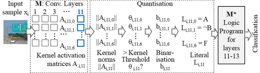
4       J. Townsend et al.

2.2   Feature importance

A lot of existing research presents ways to visualise what CNNs ‘see’ [9,10,11,12,13,14,15].
These methods generally identify the responsibility of input pixels (or neurons
in a hidden layer) with respect to activating the output neuron corresponding
to a given class. This usually involves tracing the signal back from that output
neuron, backwards through the network along stronger network weights until
arriving at the input image. This signal may be the output activation [10,31], a
gradient [9,32,33] or some other metric derived from the output [13,14]. These
ideas can be used to analyse what a specific kernel responds to [10]. Further-
more, Zhou et al. show that semantic concepts can be observed from an analysis
of a kernel’s receptive field in CNNs trained to recognise scenes, and that kernels
tend to have more semantic meaning at deeper network layers [22]. In related
work Simon et al provide a means of localising semantic parts of images [34].

2.3   Rule extraction from CNNs

Compared with methods for visualising important features as in section 2.2,
methods that model the relationships between these features are relatively few.
    Chen et al. introduce an XBD-model that includes a prototype layer that
is trained to recognise a set of prototype components so that images can be
classified by reference to these component parts. In other words, the CNN is
trained to classify images in a human-like manner. For example, one kernel
learns the concept of wing, another learns the concept of beak, and when an
input image is classified the explanation can be given as wing ∧ beak → bird.
    The prototype method, and currently our own, assumes a one-to-one rela-
tionship between kernels and symbols. However it has been observed that this
may not be the case [35]. It may be that the relationship between kernels and
semantic concepts is in fact many-to-many. Zhang et al. disentangle concepts
represented in this way and represent disentangled concepts and their relation-
ship to each other in a hierarchical graph in which each layer of the hierarchy
corresponds to a layer of the CNN [19,20]. However, the disentangled graphs
in their current form show limited expressivity in that explanations are only
composed of positive instances of parts. We extract rules in which conditions
may be positive or negative. The work was extended to an XBD approach in
which a CNN is trained with a loss function that encourages kernels to learn
disentangled relations [23], and this was then used to generate a decision tree
based on disentangled parts learned in the top convolutional layer [21].
    Bologna and Fossati extract propositional rules from CNNs [18]. First they
extract rules that approximate the dense layers, with antecedents corresponding
to the outputs of individual neurons in the last convolutional layer, and then
extract rules that summarise the convolutional layers, with antecedents mapped
to input neurons. This work is to some extent XBD as it assumes that some layers
of the original model are discretised. Only the dense layer rules are actually used
for inference, with convolutional rules only used to provide explanations. The
complexity of working with invdidual neurons as antecedents is cited as the
ERIC: Extracting Relations Inferred from Convolutions 5
Fig. 1. ERIC Pipelines for inference and rule extraction.
reason for this decision. Other work described above (and ours) overcomes this
by mapping symbols to groups of neurons (e.g. prototype kernels or disentangled
parts). One advantage over the disentanglement method is that extracted rules
may include negated antecedents.
3 ERIC Architecture
ERIC is a global explanation method that extracts rules conditioned on posi-
tive and negative instances of quantised kernel activations and is able to extract
these rules from multiple convolutional layers. ERIC assumes CNNs have stan-
dard convolution, pooling and dense layers, and is indifferent with respect to
whether the CNN has been trained with explainability in mind. ERIC is mostly
decompositional in that rules explain kernel activations but partly pedagogical
in that we only decompose a subset of convolutional layers and the output dense
layer, and treat remaining layers as black boxes. Fig. 1 presents an overview of
the architecture as two pipelines sharing most modules. We explain the inference
module first in section 3.2 in order to formalise the target behaviour of extracted
programs. All modules of the extraction pipeline are explained in section 3.3.
3.1 Preliminaries
Let us consider a set of input images x indexed by i and a CNN M whose layers
are indexed by l = 1, . . . , lo . Every layer has kernels indexed by k = 1, . . . , Kl .
Ai,l,k ∈ Rh×w denotes an activation matrix output for a kernel, where h, w are
natural numbers. Note that we treat the term kernel as synonymous with filter
and we do not need to consider a kernel’s input weights for our purposes in this
paper. Let o refer to the softmax layer at the output of M , with index lo . Let
lLEP denote the index of a special layer we call the Logical Entry Point, the
layer after which and including we approximate kernel activations.
Let bi,l,k ∈ {1, −1} denote a binary truth value associated with Ai,l,k as in eq.
1 and 2. bi,l,k may be expressed as positive and negative literals Li,l,k ≡ (bi,l,k =
1) and ¬Li,l,k ≡ (bi,l,k = −1) respectively. A set of rules indexed by r at layer l6 J. Townsend et al.
Fig. 2. Inference: kernel outputs at a designated layer are quantised and input to a
logic program that approximates remaining layers. Input sample from Places365 [36].
is denoted Rl = {Rl,r = (Dl,r , Cl,r )}r , where Dl,r and Cl,r are sets of conjoined
literals in the antecedents (conditions for satisfying the rule) and consequents
(outcomes) of Rl,r respectively. For example, Dl,r = Li,l−1,3 ∧ ¬Li,l−1,6 ∧ Li,l−1,7
and Cl,r = Li,l,2 ∧ Li,l,3 ∧ Li,l,5 . Cl,r may only contain positive literals as we
assume default negation, i.e. by default all bi,l,k = −1 (¬Li,l,k ) unless some Cl,r
determines otherwise.
3.2 Inference
Inference is summarised in fig. 2. Eq. 1 and 2 formalise the process by which
we infer a binary approximation bi,l,k for activation tensor Ai,l,k for any kernel.
An extracted program approximates convolutional layers after and including
layer lLEP , at which point kernel activations are mapped to binary values via
a quantisation function Q(Ai,l,k , θl,k ) so that these activations may be treated
as the input to logic program M ∗ (eq. 1). Q(Ai,l,k , θl,k ) is explained in detail
later in subsection 3.3. The truths of all kernels in all following layers (bi,l,k for
l > lLEP ) are derived through logical inference on the truths of binarised kernels
from the previous layer bi,l−1 according to a set of layer-specific rules Rl (eq. 2).
bi,lLEP ,k = Q(Ai,lLEP ,k , θlLEP ,k ) (1)
(
1 depending on Cl,r for all k if ∃r(Dl,r = T rue)
bi,l,k = (2)
−1 otherwise (default negation)
3.3 Rule extraction
Rule extraction is implemented as a pipeline of 5 modules (fig. 1). First is the
original model M for which we want to extract an approximation M ∗ . We do
not need to say much about this except that ERIC assumes M has already
been trained. Next in the quantisation stage we obtain binarisations for all
kernels after and including layer lLEP based on activations obtained for training
data. We then extract rules which describe the relationship between kernelsERIC: Extracting Relations Inferred from Convolutions 7
by reference to their binarisations. Then to interpret the meanings of individual
kernels we first visualise each kernel as one or more images that represent what
inputs the kernels strongly react to, before each kernel is assigned a label based
on manual inspection, a process we plan to automate in future work.
Quantisation Our quantisation function Q is defined in eq. 3, where θl,k is a
kernel-specific threshold and norm function k · k is the l1 norm1 . Intuitively, we
say that a kernel is active when its norm breaches a threshold specific to that
kernel. Note that for the initial rule extraction process we quantise all extractable
layers l ≥ lLEP but for inference we only need to quantise kernels at lLEP .
(
1 if kAi,l,k k > θl,k
Q(Ai,l,k , θl,k ) = (3)
−1 otherwise
We define a kernel’s threshold as the mean norm of its activations with respect
to the training data xtr , as in eq 4. To this end we make a forward pass of xtr in
order to obtain {Atr i,l,k }i,l,k , activations for each kernel 1 ≤ k ≤ Kl at each layer
lLEP ≤ l < lo for each input training sample 1 ≤ i ≤ n.
Pn tr
i=1 kAi,l,k k
θl,k = (4)
n
We can now use the quantisation function (eq. 3) to obtain binarisations of
all kernel activations according to eq. 5. Where a convolutional layer outputs
to a pooling layer, we take Ai,l,k from the pooled output. As also shown in eq.
5, we also need to treat output neurons as kernels of dimension 1 × 1 so that
btr tr
i,lo = M (xi ). This enables us to extract rules that map kernel activations at
layer lo − 1 to the output classifications as inferred by M .
(
otr
i,k if l = l
o
bi,l,k = (5)
Q(Atri,l,k ) otherwise
Rule extraction We now extract rules that describe the activation at each
kernel at every layer l given activations at layer l − 1. Thus, the following is
applied layer-wise from lo to lLEP . We use a tree-based extraction algorithm
similar to the C4.5 algorithm [37] to extract rules which describe conditions for
which each kernel evaluates as true. As we assume default negation, we do not
need to extract rules that describe when a kernel is false. Let us denote the
training data Zl = {(z i , ti ) | i = 1, ..., n} where z i ∈ {T rue, F alse}2Kl−1 and
ti ∈ {T rue, F alse}. Note that the length of z l is twice the number of kernels at
layer l − 1 because each kernel has positive and negative literals. zl−1,k0 = T rue
if it corresponds to a positive literal and its binary value is 1 or if it represents
a negative literal and its binary value is -1. It is False otherwise. C4.5 generates
a decision tree up to maximum depth d. Each path from the root of the tree to
1
Preliminary experiments found that l1 norm yielded higher fidelity than l2 norm.8 J. Townsend et al.
a leaf node represents a separate rule and nodes branch on rule conditions (i.e.
antecedents). The maximum number of antecedents per rule is equal to d+1. C4.5
uses entropy as a branch selection criterion but based on a marginal improvement
in fidelity observed in preliminary tests we chose to use gini index. Extraction
can become intractable as more layers and therefore kernels are introduced due
to combinatorial explosion. This can be moderated by reducing d or increasing
another parameter α that we introduce for this purpose. Let P, Q represent sets
of training instances that satisfy the path of conditions leading to a parent node
and child node, respectively. We stop branching if |Q|/|P | < α. If a leaf node
represents multiple outcomes, we set the consequence to the modal value of Q.
Finally, we simplify extracted programs by merging rules with complementary
literals (A ∧ B → C and A ∧ ¬B → C become A → C) and rules with identical
antecedents but different consequents (A → B and A → C become A → B ∧ C).
Kernel visualisation and labelling To visualise what a kernel sees, we select
the m images from xtr which activate that kernel most strongly with respect to
kAtr m
i,l,k k. We denote this visualisation as x̂l,k . A label is assigned to a kernel based
m
on x̂l,k , which for the time being we do manually based on visual inspection but
in future work plan to automate. For the time being, to defend the arguments
of the paper, it is not so much the labels that are important as the distinction
between the subsets of image that each kernel responds most strongly to.
4 Experiments
In sections 4.1 and 4.2 we outline the classification task and CNN configuration
we use for our experiments. We then extract rules from a single convolutional
layer in section 4.3 and then multiple convolutional layers in section 4.4. In
section 4.5 we visualise and label kernels and in section 4.6 analyse some of the
rules with these labels assigned to the antecedents.
4.1 Task
We chose to classify road scenes from the places365 dataset [36] for a number of
reasons. First, we felt that a scene dataset was appropriate as scenes can easily
be described by reference to symbolic entities within them which themselves
could be described by a separate classifer (i.e. the kernel classifier) with a large
vocabulary of labels. We selected a handful of 5 scenes to simplify the task
given the complexity of rule extraction, and opted for roads in order to create
a scenario where the distinction between scenes is particularly important (due
to regulations, potential hazards, etc). We wanted to demonstrate ERIC on a
multi-class task and on multiple combinations of class. 3 is the minimum required
for multi-class case and gives us 53 = 10 combinations of scenes (table 1).
ERIC: Extracting Relations Inferred from Convolutions             9

Table 1. Accuracies of the original model M and extracted program M ∗ , with the
number of unique variables (positive or negative literals) and rules for each M ∗ , and
the size of M ∗ measured as the total number of antecedents across all rules. Results are
shown for all sets of 3/5 classes: Desert road, Driveway, Forest, Highway and Street.

                    Original M        Program M ∗       M − M∗             M ∗ stats
         Classes   Train Val. Test   Tr. Val. Te.     Tr. Val. Te.     Vars Rules Size
         De,Dr,F   98.5 88.5 90.2    83.5 79.7 81.6   15.0 8.8 8.6      50    31 171
         De,Dr,H   97.5 82.7 83.6    77.2 73.5 75.0   20.3 9.2 8.6      44    32 176
         De,Dr,S   99.6 92.9 93.3    78.7 74.9 76.1   20.9 18.0 17.2    44    34 183
         De,F,H    95.0 80.8 81.5    85.0 80.7 81.4   10.0 0.1 0.1      48    36 196
         De,F,S    99.0 94.8 94.7    91.0 89.4 90.3   8.0 5.4 4.4       33    25 127
         De,H,S    97.7 84.9 86.2    80.6 78.0 78.7   17.1 6.9 7.5      42    36 194
         Dr,F,H    96.9 82.5 83.0    83.3 80.0 81.0   13.6 2.5 2.0      47    31 167
         Dr,F,S    97.9 89.7 90.9    73.4 68.9 69.6   24.5 20.8 21.3    47    33 181
         Dr,H,S    99.0 88.0 88.1    79.8 76.7 78.0   19.2 11.3 10.1    47    36 197
         F,H,S     97.7 86.9 87.1    73.8 71.2 71.6   23.9 15.7 15.5    56    34 185

      Fig. 3. Original CNN accuracy compared to accuracy of extracted model M ∗

4.2     Network Model

For each combination of classes we train VGG16 (as defined for Tensorflow using
Keras [38]) from scratch over 100 epochs using Stochastic Gradient Descent, a
learning rate of 10−5 , categorical crossentropy and a batch size of 32.

4.3     Extraction from a single layer

We set α = 0.01 so that branching stops if a branch represents less than 1% of
the samples represented by its parent node. We iterate the logical entry point
lLEP ∈ [Conv8 . . . Conv13] and tree depth d ∈ [1 . . . 5] and observe the effects
on accuracy, fidelity and the size of the extracted program. Size is measured as
the sum length (number of entecedents) of all rules and is our metric for inter-
pretability on the basis that larger programs take longer to read and understand.
In all figures we average over all results except the variable we iterate over.
    Fig. 3 compares the average accuracy across all depths and layers for each
class combination with the accuracy of the original model. The line of best fit
shows that the accuracy of the extracted model is consistent with respect to that
10 J. Townsend et al.
Fig. 4. Accuracies, fidelities and program sizes obtained from single-layer extraction.
of the original model. In the validation set, accuracy drops by about 15% in each
case. However average validation accuracy drops by an average of 10% for the
optimal selection of depth and layer (table 1). In summary, the loss in accuracy
can be moderated by adjusting extraction parameters.
Fig. 4 shows how accuracy, fidelity and program size are affected as we ad-
just the extraction layer and tree depth. Accuracy and fidelity both improve as
tree depth (and therefore rule length) is increased, demonstrating that extrac-
tion benefits from quantising more kernels. However, the cost of this is a larger
logic program. Accuracy and fidelity both show a general increase as rules are
extracted from higher layers. This is to be expected since 1) deeper layers are
known to represent more abstract and discriminative concepts, and 2) by dis-
cretising one layer we also discard all the information encoded in any following
layers. However, there is a spike at layer 10. Layers 10 and 13 of VGG16 pass
through max-pooling filters, suggesting that pooling before quantisation may
also be beneficial to accuracy. The choice of extraction layer has small but neg-
ligible effect on program size. However in our case all extraction layers have 512
kernels and results may differ when extracting from smaller or larger layers.
Optimal validation accuracies were found for conv13 and a tree depth of 5.
Table 1 presents accuracies for all class combinations based on this configuration.
The best validation accuracy was found for Desert Road, Forest Road and Street
and table 2 shows example rules extracted for this case. Note that literals are
composed of two letters because an alphabet of A-Z is insufficient for all 512
kernels, and they can be renamed in the kernel labelling stage anyway. We carry
the optimal parameters and scenario forward for all further tests.
4.4 Extraction from multiple layers
Given the higher complexity of extracting knowledge from multiple layers at
once, we do not iterate different values for tree depth but fix it at 5. We also
increase the value of α to 0.1 to enforce stricter stopping conditions and prevent
combinatorial explosion caused by observing relations between kernels at adja-
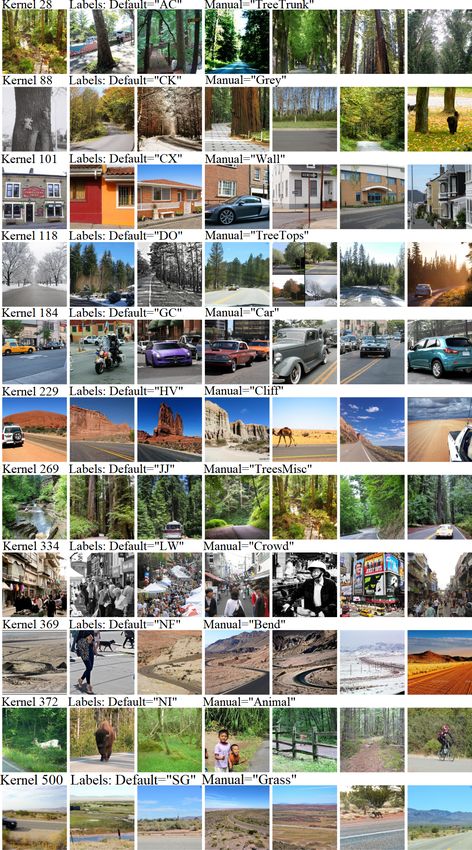
cent layers. Fig. 5 shows the effect of incrementally adding layers starting from
layer 13 only, then adding layer 12, and so on up to layer 8. Accuracy drops as
more layers are added, presumably due to an increase in information loss as moreERIC: Extracting Relations Inferred from Convolutions 11
Fig. 5. Accuracies, fidelities and program sizes yielded from multi-layer extraction.
and more kernels are quantised. Nonetheless accuracies are reasonable. However,
the size of the logic program increases exponentially as more layers are added,
emphasising the importance of adjusting d and α to moderate this.
4.5 Visualisation and labelling
It can be difficult to know which kernels to examine when inspecting large CNNs
such as VGG16 which has 512 in one layer. We have shown that using rule
extraction this number can be reduced (the best case is 33 in table 1). For now
we assign labels manually with the intention of automating this process in future
work. We label kernels represented by rules extracted for layer 13, with m = 10.
That is, we choose a kernel’s label based on the 10 images that activate it most
strongly with respect to l1 norm values obtained from a forward pass of the
training set. Fig 6 presents 7/10 images2 from x̂1013,k selected for 11 kernels.
The kernels clearly partition classes into further sub-classes with noticable
similarities within them, supporting the findings of Zhou et al. [22]. Images for
kernels 101, 184 and 334 are all taken from the street class but focus on different
things: 101 seems to focus on walls mostly free from occlusion, 184 mostly on
cars and 334 on crowds of people. Kernels 229, 369 and 500 mostly respond to
the desert class but again distinguish between different features: 229 responds
strongly to cliffs or mountains, 369 to bends in roads and 500 to desert with grass
patches. The remaining kernels respond mostly to forest images but differences
were less clear. Kernel 28 responds when tree trunks are more visible and 118
2
Limited space made it difficult to show all 10 without compromising clarity.
Table 2. 6/25 Extracted rules for classes = {desert road, forest road, street}.
1 LW ∧ ¬SG → street
7 CX ∧ ¬LW ∧ N I ∧ P O ∧ ¬SG → street
10 ¬CK ∧ DO ∧ ¬HV ∧ JB ∧ N I → f orest
13 ¬AC ∧ CK ∧ ¬DO ∧ N I ∧ ¬SG → f orest
17 ¬AC ∧ ¬DO ∧ ¬JJ ∧ SG → desert
25 AC ∧ ¬DO ∧ ID ∧ SG → desert12 J. Townsend et al.
Fig. 6. Kernel visualisations. All images from Places365 dataset [36]ERIC: Extracting Relations Inferred from Convolutions 13
Fig. 7. Misclassifications: a forest road misclassified as a desert road, a street misclas-
sified as a forest, and a forest misclassified as a street. Images from Places365 [36].
when the tree tops are visible. 88 was more difficult to choose a label for but we
chose grey due to significant grey regions in some images. 269 was also difficult
to choose for. A common feature appears to be something in the centre of the
image such as cars on two occasions, a lake on another and planks of wood in
another. It may be that the kernel has picked up on a regularity not immediatly
clear to human observers; an example of the need for a symbol for a possibly
new concept to which we assign TreesMisc as a surrogate.
However we label the kernels, the initial 3-class dataset does not have the
labels necessary to distinguish between these sub-classes even though the CNN
is capable of doing so to the extent that, as we show in sections 4.3 and 4.4, they
can be quantised and included in rules that approximate the CNN’s behaviour.
4.6 Test images
We now inspect some of the explanations given for classifications made on the
test set, assigning the labels in fig. 6 to the rules in table 2. Rule 1 translates
as Crowd ∧ ¬Grass → street, i.e. “if you encounter people and no grass then
you are in a street”. Of course, in reality there are other situations where people
may be found without grass, and some empty streets may have grass patches, so
we as humans would not conclude we are in a street with this information alone.
However, in this particular “Desert, Forest or Street” case on which the CNN
was trained, one is significantly less likely to encounter people in the former two
categories. Thus, this is enough information for the CNN to identify the location.
Rule 7 translates as Grey ∧ T reeT ops ∧ Animal → f orest. Animals may appear
in streets, as would a grey surface, but when they appear together with trees it
is more likely to be a forest. Rule 17 translates as ¬T reeT runk ∧ ¬T reeT ops ∧
¬T reesM isc ∧ Grass → desert, i.e. “if there is grass but no trees then it must
be a desert”. Again, there are many places with grass but no trees (e.g. a field)
but in this particular task the CNN has no other concept of grass without trees.
Fig. 7 shows three images for which both the original and approximated
models made identical misclassifications. In the first example rule 17 misclassifies
a forest road as a desert road. Although trees are present they are perhaps
too few to activate the tree-related kernels, satisfying the negated tree-based
antecedents. Grass by the road satisfies the other antecedent. In the second
case rule 10 (T reeT runk ∧ ¬W all ∧ T reeT ops ∧ ¬Crowd ∧ ¬Animal → f orest)14 J. Townsend et al.
confuses a street for a forest road as there are no animals in the street and
many trees occlude the walls of the houses. The image from the forest set is
misclassified as a street according to rule 1 as there are people and no grass.
5 Discussion and future work
ERIC quantises the outputs of kernels in a CNN and relates these kernels to each
other as logical rules that yield lower but reasonable accuracy. Our inspection
of these kernels supported existing findings that most exhibit a strong response
to sets of similar images with common semantic features [22]. We hope to au-
tomate the process of labelling these symbols in future work, likely integrating
existing methods for mapping kernels or receptive fields to semantic concepts
[34,22,19,20]. However these methods have finite sets of labels originally pro-
vided by humans with finite vocabularies. It may be that knowledge extraction
methods will find new and important symbols for which we need to invent new
words. ERIC provides a framework for discovering symbols that are important
enough to distinguish between classes but for which no labels yet exist.
Although the rules in section 4.6 are not paths of reasoning humans are likely
to take, they nonetheless suffice to approximate the behaviour of the original
CNN. It would be unreasonable for a human to assume they are in a street just
because they see people and no grass, but for a CNN that has only seen streets,
forests and desert roads, it is a reasonable assumption. Being able to explain
how a machine ‘thinks’ does not necessarily mean that it thinks like a human.
An empirical comparison of performance of methods listed in the background
also remains to be addressed in future work, but for now we comment on how
they differ in terms of features. ERIC is a global explanation model that extracts
rules in which antecedents are composed of positive and negative instances of
quantised kernel activations, and is able to extract these rules from multiple
convolutional layers. ERIC lacks some features that may be of benefit such as
the ability to disentangle features and thus overcome assumptions regarding one-
to-one relationships between kernels and concepts. However relationships defined
using the disentanglement method do not include negated symbols as ERIC does.
Both methods have potentially mutually beneficial features and adapting ERIC
to disentangle representations would be an interesting future step.
Finally, although ERIC is not yet compatible with architectures designed for
explainability, we expect it would be compatible with weight matrices that have
been trained for explainability. We would like to test this hypothesis and use
ERIC as a framework for assessing how this affects fidelity and explainability.
6 Conclusions
We have shown that the behaviour of kernels across multiple convolutional layers
can be approximated using a logic program, and the extracted program can be
used as a framework in which we can begin to understand the behaviour of
CNNs and how they think. More specifically, it can be used to identify kernelsERIC: Extracting Relations Inferred from Convolutions 15
worthy of deeper inspection and their relationships with other kernels in the
form of logical rules. Our own inspections show that the kernels in the last
convolutional layer may be associated with concepts that are symbolic in the
sense that they are visually distinct from those represented by other kernels.
Some of these symbols were more interpretable from a human perspective than
others. However regardless of what labels we assign, we have shown that these
kernels can be used to construct symbolic rules that approximate the behaviour
of the CNN to an accuracy that can be improved by adjusting rule length and
the choice of layer or layers to extract from, at the cost of a larger and therefore
less interpretable but nonetheless symbolic logic program. In the best case, we
saw an average 10% drop in accuracy compared with the original model.
References
1. Ribeiro, M.T., Singh, S., Guestrin, C.: Why should I trust you?: Explaining the pre-
dictions of any classifier. In: Proceedings of the 22nd ACM SIGKDD International
Conference on Knowledge Discovery and Data Mining, ACM (2016) 1135–1144
2. Gilpin, L.H., Bau, D., Yuan, B.Z., Bajwa, A., Specter, M., Kagal, L.: Explaining
explanations: An overview of interpretability of machine learning. In: 2018 IEEE
5th International Conference on Data Science and Advanced Analytics (DSAA),
IEEE (2018) 80–89
3. Guidotti, R., Monreale, A., Ruggieri, S., Turini, F., Giannotti, F., Pedreschi, D.:
A survey of methods for explaining black box models. ACM computing surveys
(CSUR) 51 (2018) 93
4. Andrews, R., Diederich, J., Tickle, A.B.: Survey and critique of techniques for
extracting rules from trained artificial neural networks. Knowledge-based systems
8 (1995) 373–389
5. Jacobsson, H.: Rule extraction from recurrent neural networks: A taxonomy and
review. Neural Computation 17 (2005) 1223–1263
6. Townsend, J., Chaton, T., Monteiro, J.M.: Extracting relational explanations from
deep neural networks: A survey from a neural-symbolic perspective. IEEE trans-
actions on neural networks and learning systems (2019)
7. Zhang, Q., Zhu, S.: Visual interpretability for deep learning: a survey. Frontiers
of Information Technology & Electronic Engineering 19 (2018) 27–39
8. Lamb, L., Garcez, A., Gori, M., Prates, M., Avelar, P., Vardi, M.: Graph neu-
ral networks meet neural-symbolic computing: A survey and perspective. arXiv
preprint arXiv:2003.00330 (2020)
9. Simonyan, K., Vedaldi, A., Zisserman, A.: Deep inside convolutional net-
works: Visualising image classification models and saliency maps. arXiv preprint
arXiv:1312.6034 (2013)
10. Zeiler, M.D., Fergus, R.: Visualizing and understanding convolutional networks.
In: European conference on computer vision, Springer (2014) 818–833
11. Springenberg, J.T., Dosovitskiy, A., Brox, T., Riedmiller, M.: Striving for simplic-
ity: The all convolutional net. arXiv preprint arXiv:1412.6806 (2014)
12. Bojarski, M., Choromanska, A., Choromanski, K., Firner, B., Jackel, L., Muller,
U., Zieba, K.: Visualbackprop: efficient visualization of cnns. arXiv preprint
arXiv:1611.05418 (2016)16 J. Townsend et al.
13. Bach, S., Binder, A., Montavon, G., Klauschen, F., Müller, K., Samek, W.: On
pixel-wise explanations for non-linear classifier decisions by layer-wise relevance
propagation. PloS one 10 (2015) e0130140
14. Samek, W., Binder, A., Montavon, G., Lapuschkin, S., Müller, K.: Evaluating the
visualization of what a deep neural network has learned. IEEE transactions on
neural networks and learning systems 28 (2017) 2660–2673
15. Shrikumar, A., Greenside, P., Kundaje, A.: Learning important features through
propagating activation differences. arXiv preprint arXiv:1704.02685 (2017)
16. Frosst, N., Hinton, G.: Distilling a neural network into a soft decision tree. arXiv
preprint arXiv:1711.09784 (2017)
17. Chen, C., Li, O., Tao, D., Barnett, A., Rudin, C., Su, J.K.: This looks like that: deep
learning for interpretable image recognition. In: Advances in Neural Information
Processing Systems. (2019) 8930–8941
18. Bologna, G., Fossati, S.: A two-step rule-extraction technique for a cnn. Electronics
9 (2020) 990
19. Zhang, Q., Cao, R., Wu, Y.N., Zhu, S.: Growing interpretable part graphs on
convnets via multi-shot learning. In: Thirty-First AAAI Conference on Artificial
Intelligence. (2017)
20. Zhang, Q., Cao, R., Shi, F., Wu, Y.N., Zhu, S.: Interpreting CNN knowledge via an
explanatory graph. In: Thirty-Second AAAI Conference on Artificial Intelligence.
(2018)
21. Zhang, Q., Yang, Y., Ma, H., Wu, Y.N.: Interpreting cnns via decision trees. In:
Proceedings of the IEEE Conference on Computer Vision and Pattern Recognition.
(2019) 6261–6270
22. Zhou, B., Khosla, A., Lapedriza, A., Oliva, A., Torralba, A.: Object detectors
emerge in deep scene CNNs. arXiv preprint arXiv:1412.6856 (2014)
23. Zhang, Q., Nian Wu, Y., Zhu, S.: Interpretable convolutional neural networks. In:
Proceedings of the IEEE Conference on Computer Vision and Pattern Recognition.
(2018) 8827–8836
24. Percy, C., d’Avila Garcez, A.S., Dragicevic, S., França, M.V., Slabaugh, G.G.,
Weyde, T.: The need for knowledge extraction: Understanding harmful gambling
behavior with neural networks. Frontiers in Artificial Intelligence and Applications
285 (2016) 974–981
25. Ribeiro, M.T., Singh, S., Guestrin, C.: Anchors: High-precision model-agnostic
explanations. In: AAAI Conference on Artificial Intelligence. (2018)
26. Zilke, J.R., Mencı́a, E.L., Janssen, F.: Deepred–rule extraction from deep neural
networks. In: International Conference on Discovery Science, Springer (2016) 457–
473
27. Schaaf, N., Huber, M.F.: Enhancing decision tree based interpretation of deep neu-
ral networks through l1-orthogonal regularization. arXiv preprint arXiv:1904.05394
(2019)
28. Nguyen, T.D., Kasmarik, K.E., Abbass, H.A.: Towards interpretable deep neural
networks: An exact transformation to multi-class multivariate decision trees. arXiv
preprint arXiv:2003.04675 (2020)
29. Murdoch, W.J., Szlam, A.: Automatic rule extraction from long short term memory
networks. arXiv preprint arXiv:1702.02540 (2017)
30. Tran, S.N., d’Avila Garcez, A.S.: Deep logic networks: Inserting and extracting
knowledge from deep belief networks. IEEE transactions on neural networks and
learning systems (2016)ERIC: Extracting Relations Inferred from Convolutions 17
31. Zhou, B., Khosla, A., Lapedriza, A., Oliva, A., Torralba, A.: Learning deep fea-
tures for discriminative localization. In: Computer Vision and Pattern Recognition
(CVPR), 2016 IEEE Conference on, IEEE (2016) 2921–2929
32. Denil, M., Demiraj, A., De Freitas, N.: Extraction of salient sentences from labelled
documents. arXiv preprint arXiv:1412.6815 (2014)
33. Selvaraju, R.R., Cogswell, M., Das, A., Vedantam, R., Parikh, D., Batra, D.: Grad-
cam: Visual explanations from deep networks via gradient-based localization. In:
Proceedings of the IEEE international conference on computer vision. (2017) 618–
626
34. Simon, M., Rodner, E., Denzler, J.: Part detector discovery in deep convolutional
neural networks. In: Asian Conference on Computer Vision, Springer (2014) 162–
177
35. Xie, N., Sarker, M.K., Doran, D., Hitzler, P., Raymer, M.: Relating input concepts
to convolutional neural network decisions. arXiv preprint arXiv:1711.08006 (2017)
36. Zhou, B., Lapedriza, A., Khosla, A., Oliva, A., Torralba, A.: Places: A 10 million
image database for scene recognition. IEEE Transactions on Pattern Analysis and
Machine Intelligence (2017)
37. Quinlan, J.R.: C4.5: Programming for machine learning. The Morgan Kaufmann
Series in Machine Learning, San Mateo, CA: Morgan Kaufmann 38 (1993) 48
38. Chollet, F., et al.: Keras. https://github.com/fchollet/keras (2015)You can also read