Analyse Success Model of Split Time and Cut-Off Point Values of Physical Demands to Keep Category in Semi-Professional Football Players - MDPI
←
→
Page content transcription
If your browser does not render page correctly, please read the page content below
applied
           sciences
Article
Analyse Success Model of Split Time and Cut-Off
Point Values of Physical Demands to Keep Category
in Semi-Professional Football Players
Jesus Vicente Gimenez 1,2 , Luis Jimenez-Linares 3 , Jorge Garcia-Unanue 4, * ,
Javier Sanchez-Sanchez 1 , Leonor Gallardo 4 and Jose Luis Felipe 1
 1    School of Sport Sciences, Universidad Europea de Madrid, Edificio Juan Mayorga, C/Tajo, s/n, Villaviciosa de
      Odón, 28670 Madrid, Spain; intertato_@hotmail.com (J.V.G.);
      javier.sanchez2@universidadeuropea.es (J.S.-S.); joseluis.felipe@universidadeuropea.es (J.L.F.)
 2    International University of Valencia (VIU), 46002 Valencia, Spain
 3    School of Computer Science, Department of Information Technologies and Systems, University of Castilla-La
      Mancha, 13017 Ciudad Real, Spain; luis.jimenez@uclm.es
 4    IGOID Research Group, Department of Physical Activity and Sport Sciences, University of Castilla-La
      Mancha, Avenida Carlos III, s/n, Campus Tecnológico Fábrica de Armas, Laboratorio Gestión Deportiva,
      45071 Toledo, Spain; leonor.gallardo@uclm.es
 *    Correspondence: jorge.garciaunanue@uclm.es

 Received: 10 June 2020; Accepted: 29 July 2020; Published: 31 July 2020

 Abstract: The aim of this study was to analyse different success models and split time on cut-off
 point values on physical demands to keep category in semi-professional football players. An ad
 hoc observational controlled study was carried out with a total of ten (840 match data) outfield
 main players (25.2 ± 6.3 years, 1.79 ± 0.75 m, 74.9 ± 5.8 kg and 16.5 ± 6 years of football experience)
 and monitored using 15 Hz GPS devices. During 14 official matches from the Spanish division B
 in the 2016/2017 season, match data were coded considering the situational variable (score) and
 classified by match results (winning, losing or drawing). The results show significant differences
 between high-intensity attributes criteria that considered split time in velocity zones of 0–15 min
 (p = 0.043, ηp2 = 0.065, medium), 30–45 min (p = 0.010, ηp2 = 0.094, medium) and 60–75 min (p = 0.015,
 ηp2 = 0.086, medium), as well as sprint 60–75 min (p = 0.042, ηp2 = 0.066, medium) and 75–90 min
 (p = 0.002, ηp2 = 0.129, medium). Decision tree induction was applied to reduce the disparity range of
 data according to six 15-min intervals and to determine the cut-off point values for every parameter
 combination. It was possible to establish multivariate models for the main high-intensity actions
 criteria, allowing the establishment of all rules with their attributes and enabling the detection and
 visualisation of relationships and the pattern sets of variables for determining success.

 Keywords: competition analysis; GPS technology; decision tree; fuzzy set; football

1. Introduction
     Football is characterised by brief linear and non-linear efforts of high intensity alternated with
non-established periods (short or long) of recovery [1], where performance depends on different
technical, tactical, biomechanical, psychological and physiological characteristics [2]. During a
professional match, a football player covers a total distance of 9–14 km [3]. This distance is mostly
covered at a low intensity (
Appl. Sci. 2020, 10, 5299 2 of 13
where the high-intensity actions that involve accelerations and decelerations are critical points [6],
with a work:rest ratio of 1:8 [7].
There are multiple variables of the situation, such as the competitive level [8], the opponent’s
level [9], the tactical system [10], the pressure to achieve the objective [11] and the conditions, quantity
and the intensity of the efforts demanded during the competition [12]. Recently, several studies relied
on these physical demands during a football game to propose metrics that quantify specific aspects of
football performance [13–15]. This performance and their connection with competitive success (i.e.,
to win a match) have been the focus of attention in several studies [12,15,16]. Thus, a positive relation
has been found between greater physical demand and match success, i.e., for the English Premier
League [1], the Spanish La Liga [12] or elite women football players [17].
Football elite and semi-professional training generally includes tracking by GPS or different
tracking systems of workloads, movement patterns and performance [18]. This situation provides a
huge amount data about each player, team, game and season. In this context, data mining techniques
are employed to assist in decision-making [19]. Sports teams can gain advantage over their rivals by
converting data to applied knowledge through appropriate data extraction and interpretation [20].
Moreover, although various unidentified factors may influence the results, data mining will still be
valuable in result prediction [21]. To date, the use of data mining techniques to predict football success
has focused on decision tree classifiers [22]. This technique generates outcomes by repeatedly dividing
training data [23]. An important feature of this machine learning model is its ability to determine the
best threshold or cut-off point values that differentiate each training [24]. These models may be critical
in considering load-related information during football drills used by elite and semi-professional
players compared to competition match demands [25].
However, no study has yet investigated the influence of the physical performance variables on
match results using the cut-off points method. Therefore, the aim of this study was to analyse the
influence of the different physical parameters variables on match results, using cut-off points method,
in a semi-professional football team that fought to keep category.
The contribution of this study to the literature and the differences from previous studies are clear,
both in the field of machine learning applications and in the contributions to the field of performance
analysis. According to an updated review published in 2019, only one of the studies found included
physical variables for the discrimination of the results and the cut-off points, applied to basketball [26].
This study also confirms that one of the two most productive methods of machine learning are the
decision trees [26]. Previous studies that included machine learning application in soccer used as
discriminating variables the participation of star players or not [27], technical variables such as passes
or shots [28–30] or the previous results in the season [31]. A more current study is the only one found
that uses physical variables to establish cut-off points but applied to simulated games [32]. There is no
clear evidence in the use of decision tress and cut-off points with physical variables in real competitive
situations and specific situations such as the process to keep category. Therefore, this study provides a
relevant advance in knowledge, by expanding the use of decision trees with physical variables and
how it can be applied to specific competitive situations.
2. Materials and Methods
2.1. Sample
Ten male main outfield players (25.2 ± 6.3 years, 1.79 ± 0.75 m, 74.9 ± 5.8 kg and 16.5 ± 6 years
of football experience, goalkeeper excluded) participated voluntarily during 14 competition matches
until having the options to keep category in Spanish second B Division League matches. Only players
who played regularly and in the majority of official league matches were considered for the study
(i.e., the criterion for inclusion was that players had to have played more than 65 min of total playing
time during each match) [33]. All players and coaches were informed of the protocol of the study,
and participants’ signed informed consent was obtained before participating in the study. The studyAppl. Sci. 2020, 10, 5299 3 of 13
was conducted according to the requirements of the Declaration of Helsinki (2013), was approved by
the Clinical Research Ethical Committee of European University of Madrid (CIPI48/2019) and received
formal approval from the professional football club involved.
2.2. Procedures
The final sample consisted of 840 match data. All variables were recorded with a 15 Hz GPS
system, 100 Hz-10G accelerometer and 50 Hz magnetometer (GPSport, Camberra, Australia) on six
15-min split-time time measurement (i.e., 0–15, 15–30 and 30–45 min and 45–60, 60–75 and 75–90 min,
respectively). The sampled match results (7 home and 7 away matches) performance consisted of
a total of 11 goals scored and 18 conceded by the sample team (i.e., 2 wins, 5 draws and 7 losses).
Only 14 out of the total of 38 matches of the season were analysed. For this reason, the matches prior
to the 22nd match and after the 35th match, where fulfilling the aim to stay in the same division was
mathematically impossible were ignored. After performance tagging at each football match, all GPS
data were downloaded to a PC and analysed using GPS software package TeamAMS v4.0 (GPSport,
Canberra, Australia).
Data on the total distance covered during the game and the distance covered in each speed range
zone were calculated according to previous studies [11,34]: standing (Z1; 0–2 km/h); walking (Z2;
2–7 km/h); easy running (Z3; 7–13 km/h); fast running (Z4; 13–18 km/h); high-speed running (Z5;
18–21 km/h); and sprinting (Z6; >21 km/h). Actions above (Z5–Z6) 18 km/h were considered for this
study as high-intensity running. The GPS system also provided information about the number, time
and distance of the sprints. Moreover, GPS devices registered the maximum acceleration peaks and the
number of accelerations of the players in different ranges of intensity used in previous research [35]
and adapted to the semi-professional football players [11]: Zone 1, 1.5–2 m/s2 ; Zone 2, 2–2.5 m/s2 , Zone
3, 2.5–2.75 m/s2 ; and Zone 4, >2.75 m/s2 .
Matches were classified in function to outcome to identify the dimensions of physical performance
having a membership value (0 scored= (0) zero point of success; 2 scored= (1/3) of success;
and 3 scored = (1) one point of success). Fuzzy set “Success” is defined over the domain 0 to
|C|*3 of possible points for the set of matches C and a membership function as: [success (C) = point
(C)/(|C|)*3]. Generalise the function’s success described above with W (number of win matches),
D (number of drawn matches) and L (number of lost matches). Therefore, |C| = W + D + L, and success
is achieved when |C| = (Aw*W + AD*D + AL*L)/(AW*|C|), with Aw the value for winning match,
AD drawing match and AL losing match, such that Aw < AD < AL [36]. The mathematics member
function of fuzzy set Success was determined by:
C = p0 , p1 , . . . , pr pi ∈ {win, draw, loss}
3 p = win
Val(p) = 2 p = draw
0 p = loss
P
p∈C val(p)
Succes(C) =
val(win) ∗ |C|
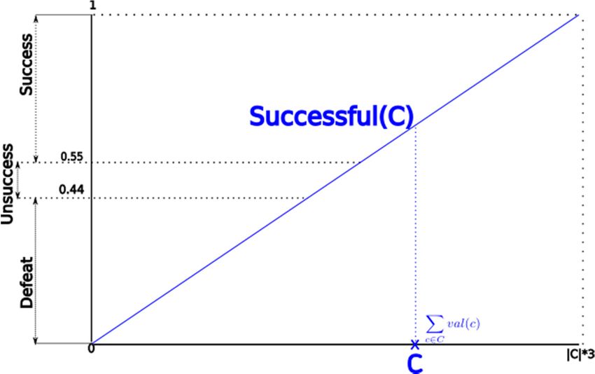
Knowing that the attribution of success and failure is difficult to define and depends on the
subject’s perspective [37], and in accordance with the approaches used in previous research [38],
we propose the segmentation of the level of success, measured with the membership function if fuzzy
set of success, with three labels: Success (S), Defeat (D) and a third intermediate one (not success, U)
DEFEAT success(C) ≤ 0.44
0.44 < success(C) < 0.55
label(success(C)) = UNSUCCESS
SUCCESS success(C) ≥ 0.55Appl. Sci. 2020, 10, 5299 4 of 13
In the end, the sample was divided taking into consideration this situational variable (score),
classified by the match result (winning, losing or drawing) and divided by the six split-time time
measurements mentioned above.
2.3. Statistical Analysis
Appl. Sci. 2020, 10, x FOR PEER REVIEW 4 of 14
To investigate the effect of the cut-off point values that best differentiate the split time on the
physical demands
To investigate theineffect
competition, data normality
of the cut-off point valueswas confirmed
that via the Shapiro–Wilk
best differentiate the split timetest
on(p > physical
the 0.05).
Comparisons among success, unsuccess and defeat were performed using
demands in competition, data normality was confirmed via the Shapiro–Wilk test (p > 0.05). Comparisonsa one-way ANOVA and
post success,
among hoc analysis (p < 0.05).
unsuccess andThe proportion
defeat of the total
were performed variability
using a one-way attributable
ANOVA toand
a factor
postwas
hocestimated
analysis (p <
via effect size using the partial Eta-squared (ηp 2 ) value with the following interpretation: small
0.05). The proportion of the total variability attributable to a factor was estimated via effect size using the
partial = 0.01–0.059);
(ηp2Eta-squared (ηpmedium
2) value(ηp with=the
2 − 0.14); and
0.06following large effect (ηp
interpretation: small>(ηp
2 0.14).
2 = 0.01–0.059); medium (ηp2 =
The decision
0.06- 0.14); and largetree,
effectgenerated with the ID3 algorithm using a gain ratio criterion, was the tool
(ηp2 > 0.14).
selected
The decision tree, generated with thethe
to reduce the disparity within range
ID3 of datausing
algorithm (i.e., toa minimise
gain ratioentropy)
criterion,[22]
wasand
thetotool
describe
selected
the physical performances of the team football players [18]. To establish the cut-off
to reduce the disparity within the range of data (i.e., to minimise entropy) [22] and to describe the physical point values
according to
performances ofsix
the15-min intervals,
team football a classifier
players model
[18]. To was the
establish used [39]. To
cut-off process
point valuescut-off point to
according values of
six 15-min
the match, the dataset was analysed using Rapidminer studio v. 8.1 (RapidMiner,
intervals, a classifier model was used [39]. To process cut-off point values of the match, the dataset was Inc. Headquarters,
Boston,using
analysed MA,Rapidminer
USA). Finally, the cut-off
studio point in relation
v. 8.1 (RapidMiner, Inc. to temporal split-time
Headquarters, Boston, with
MA, three
USA).linguistic
Finally, the
labels was determined (Figure 1).
cut-off point in relation to temporal split-time with three linguistic labels was determined (Figure 1).
Figure 1. Labelling mapping of membership function of fuzzy set Successful.
3. Results
3. Results
Significant
Significant differences
differences werewerefoundfound in distance
in total total distance
covered covered
in splitsin0–15,
splits 0–15,
30–45 30–45
and and
60–75, 60–75,
where more
where more metres are covered in defeat matches (p < 0.05). Furthermore, many sprints
metres are covered in defeat matches (p < 0.05). Furthermore, many sprints were shown in defeat matches were shown in
defeat
in the matches
splits in the
60–75 and splits(p60–75
75–90 and
< 0.05). The75–90 (p < 0.05).
descriptive andThe descriptive
statistical and statistical
inference inference
results for resultsand
each variable
for each variable and split
split time are presented in Table 1.time are presented in Table 1.Appl. Sci. 2020, 10, 5299 5 of 13
Table 1. Differences between results by split time.
Success Unsuccess Defeat p η2
M ± SD CI95% M ± SD CI95% M ± SD CI95%
0–15 1534.85 ± 179.35 1426.47 - 1643.23 1560.78 ± 192.36 1497.55 - 1624.00 1658.52 ± 216.19 1593.57 - 1723.47 0.043 0.065
Distance covered (m)
15–30 1547.12 ± 110.58 1480.29 - 1613.94 1537.24 ± 181.96 1477.43 - 1597.05 1652.11 ± 777.89 1418.41 - 1885.82 0.606 0.011
30–45 1541.16 ± 123.14 1466.75 - 1615.58 1442.35 ± 176.41 1384.36 - 1500.33 1563.40 ± 196.68 1504.31 - 1622.49 0.010 0.094
45–60 1477.44 ± 154.99 1383.78 - 1571.10 1500.49 ± 157.38 1448.76 - 1552.22 1575.25 ± 185.52 1519.51 - 1630.99 0.069 0.056
60–75 1384.82 ± 280.54 1215.29 - 1554.35 1440.79 ± 165.60 1386.36 - 1495.22 1541.24 ± 197.46 1481.92 - 1600.57 0.015 0.086
75–90 1183.85 ± 389.05 948.75 - 1418.94 1415.76 ± 175.31 1358.13 - 1473.38 1402.68 ± 184.70 1347.19 - 1458.18 0.114 0.102
Accelerations (n)
0–15 5.15 ± 1.91 4.00 - 6.31 5.61 ± 2.82 4.68 - 6.53 6.13 ± 3.24 5.16 - 7.11 0.504 0.015
15–30 4.31 ± 1.38 3.48 - 5.14 5.13 ± 2.08 4.45 - 5.82 5.53 ± 4.85 4.08 - 6.99 0.555 0.013
30–45 4.46 ± 2.93 2.69 - 6.23 5.13 ± 2.88 4.19 - 6.08 5.69 ± 2.07 5.07 - 6.31 0.271 0.028
45–60 4.38 ± 2.75 2.72 - 6.05 5.82 ± 2.89 4.86 - 6.77 5.11 ± 2.46 4.37 - 5.85 0.212 0.033
60–75 4.08 ± 2.25 2.72 - 5.44 5.18 ± 2.23 4.45 - 5.92 4.73 ± 2.45 4.00 - 5.47 0.322 0.024
75–90 3.38 ± 2.60 1.81 - 4.96 4.82 ± 3.17 3.77 - 5.86 4.20 ± 2.24 3.53 - 4.87 0.235 0.031
Decelerations (n)
0–15 3.08 ± 2.43 1.61 - 4.55 2.97 ± 2.20 2.25 - 3.70 3.16 ± 2.41 2.43 - 3.88 0.939 0.001
15–30 3.54 ± 2.44 2.07 - 5.01 3.05 ± 1.77 2.47 - 3.63 3.49 ± 3.82 2.34 - 4.64 0.772 0.006
30–45 2.62 ± 1.45 1.74 - 3.49 3.18 ± 1.84 2.58 - 3.79 3.11 ± 2.16 2.46 - 3.76 0.654 0.009
45–60 2.46 ± 1.13 1.78 - 3.14 2.68 ± 1.66 2.14 - 3.23 3.38 ± 2.17 2.73 - 4.03 0.141 0.041
60–75 2.15 ± 1.68 1.14 - 3.17 2.97 ± 1.79 2.38 - 3.56 3.38 ± 1.99 2.78 - 3.98 0.116 0.045
75–90 2.15 ± 1.82 1.05 - 3.25 2.32 ± 1.77 1.73 - 2.90 2.53 ± 1.73 2.01 - 3.05 0.741 0.006
0–15 2.92 ± 2.47 1.43 - 4.41 3.13 ± 2.16 2.42 - 3.84 3.38 ± 2.23 2.71 - 4.05 0.774 0.005
Sprints (n)
15–30 2.46 ± 2.07 1.21 - 3.71 3.21 ± 1.89 2.59 - 3.83 3.62 ± 3.03 2.71 - 4.53 0.332 0.023
30–45 2.85 ± 2.15 1.54 - 4.15 3.03 ± 1.99 2.37 - 3.68 3.20 ± 2.52 2.44 - 3.96 0.868 0.003
45–60 2.77 ± 2.20 1.44 - 4.10 3.21 ± 2.47 2.40 - 4.02 3.11 ± 2.10 2.48 - 3.74 0.833 0.004
60–75 2.08 ± 1.75 1.02 - 3.14 3.21 ± 2.11 2.52 - 3.90 3.69 ± 1.99 3.09 - 4.29 0.042 0.066
75–90 1.08 ± 1.12 0.40 - 1.75 3.08 ± 2.02 2.42 - 3.74 3.22 ± 1.94 2.64 - 3.81 0.002 0.129Appl. Sci. 2020, 10, 5299 6 of 13
A result of the movement patterns derived by the participating individuals of player was classified
into Appl.
three Sci.models
2020, 10, x for FOR the
PEERdifferent
REVIEW criteria considered (i.e., zones of velocity, sprint and6 acceleration of 14
and deceleration number). It generated three decision trees for every criterion variable with regard to
A result of the movement patterns derived by the participating individuals of player was classified
six 15-min intervals (I; 1 to 6), ranging from 0–90 min to the identified cut-off values in relation to the
into three models for the different criteria considered (i.e., zones of velocity, sprint and acceleration and
mineddeceleration times
six split number). thatIt differentiated
generated three the factors
decision trees offorwin, draw
every and lost
criterion in competitive
variable with regard to matches.
six
A decision
15-min intervals tree (I;was created
1 to 6), ranging(Figure from 0–90 2)min
categorising
to the identified work rate values
cut-off movement patterns
in relation into six speed
to the mined
sixranging
zones, split times from 0 to >21.0 km·h
that differentiated −1 Theofattributes
the factors win, draw were and lost in competitive
codified matches. into 16 [root nodes
hierarchically
(RNs) 1–16], which could conduct the performed (cut-off) in each split time intointo
A decision tree was created (Figure 2) categorising work rate movement patterns six speedStatistical
16 levels.
zones, ranging from 0 to >21.0 km·h⁻¹ The attributes were codified hierarchically into 16 [root nodes
tendency for differences showed: Success (S1,2,3,6,8,9,12,13,14 ), Unsuccess (U4 ) and Defeat (D5,7,10,11,15,16 ).
(RNs) 1–16], which could conduct the performed (cut-off) in each split time into 16 levels. Statistical
However,
tendency thefor number-sprint
differences showed: abilities decision
Success tree (Figure
(S1,2,3,6,8,9,12,13,14 3) was(Ucharacterised
), Unsuccess inducing sprinting
4) and Defeat (D5,7,10,11,15,16).
performance
However,during match playabilities
the number-sprint according to attributes,
decision tree (Figure which
3) waswere codified hierarchically
characterised into 12 (RNs
inducing sprinting
1–12), which could
performance during conduct
match playthe according
performed cut-off in
to attributes, eachwere
which split time into
codified of 12 levels.
hierarchically into 12The
(RNsstatistical
1–12), was:
tendency which Success
could conduct the performed
(S1,6,7,10,11,12 cut-off in
), Unsuccess (Ueach split time into of 12 levels. The statistical
3 ) and Defeat (D2,4,5,8,9 ). Finally, the number of
tendency was: Success (S 1,6,7,10,11,12), Unsuccess (U3) and Defeat (D2,4,5,8,9). Finally, the number of
accelerations and decelerations decision tree (Figure 4) was labelled into profile markers’ capacity
accelerations and decelerations decision tree (Figure 4) was labelled into profile markers’ capacity
during match play and were codified hierarchically into 10 (RN 1–10), which could conduct the
during match play and were codified hierarchically into 10 (RN 1–10), which could conduct the
performed
performed cut-off
cut-off in in
each
eachsplit
split time into10
time into 10levels.
levels. The The statistical
statistical tendency
tendency for differences
for differences showed: showed:
Success (S2,5,6,9,10
Success (S2,5,6,9,10),),Unsuccess
Unsuccess (U (U4,8)4,8
and) and Defeat
Defeat (D1,3,7(D). 1,3,7 ).
Figure 2. Final decision tree categorised into six speed zones (km/h) including 16 Roots Nodes and
Figure 2. Final decision tree categorised into six speed zones (km/h) including 16 Roots Nodes and 3
3 rules
Appl. (i.e., Success,
Sci. 2020, Unsuccess
10, x FOR and Defeat).
PEER REVIEW 7 of 14
rules (i.e., Success, Unsuccess and Defeat).
Figure 3.Figure
Final3. Final decision
decision tree
tree categorised into
categorised intonumber
numbersprint abilities
sprint including
abilities 12 Root Nodes
including and Nodes
12 Root 3 rules and
(i.e., Success, Unsuccess and Defeat).
3 rules (i.e., Success, Unsuccess and Defeat).Figure 3. Final decision tree categorised into number sprint abilities including 12 Root Nodes and 3 rules
(i.e., Success, Unsuccess and Defeat).
Appl. Sci. 2020, 10, 5299 7 of 13
Figure
Figure4.4.Final
Finaldecision
decisiontree
treecategorised
categorised into
into number accelerations and
number accelerations anddecelerations
decelerationsincluding
including1010Root
Root
Nodes
Nodesand
and33rules
rules(i.e.,
(i.e.,Success,
Success,Unsuccess
UnsuccessandandDefeat).
Defeat).
InInaddition
additiontotoattributes
attributeswhich
whichcould
could bebe
categorised
categorised to to
thethe
three labels
three (i.e.,
labels Success,
(i.e., Unsuccess
Success, and
Unsuccess
Defeat) through
and Defeat) theirtheir
through nodes, fuzzy
nodes, success
fuzzy successsetset
waswasapplied
appliedtotothe
the gradual assessment
assessment of ofnodes
nodes
membership
membershipininthe thereal
realunit
unitinterval
interval[0,1] taking
[0, 1] takinginto account
into accountthat some
that information
some information is incomplete, and
is incomplete,
inand
particular the statistical
in particular distributions
the statistical (Table
distributions 2). 2).
(Table
Table 2. Fuzzy success set with rules interpretation and Label G for physical demands.
Speed Zones (km·h−1 ) Sprint (n) Acceleration and Deceleration (n)
Nodes
Success (%) Label G Success (%) Label G Success (%) Label G
1 0.93 * S 0.67 * S 0.00 D
2 0.67 * S 0.00 D 0.67 * S
3 1* S 0.50 † U 0.05 D
4 0.50 † U 0.36 D 0.51 † U
5 0.00 D 0.00 D 0.89 * S
6 0.64 * S 0.83 * S 0.75 * S
7 0.25 D 1* S 0.30 D
8 0.67 * S 0.26 D 0.55 † U
9 0.67 * S 0.33 * D 0.94 * S
10 0.00 D 1* S 0.67 * S
11 0.00 D 0.83 * S
12 0.86 * S 0.67 * S
13 0.67 * S
14 0.67 * S
15 0.00 D
16 0.00 D
Note: Label G: interpretation; * Success (S) = ≥ 0.55; † Unsuccess (U) = > 0.44 to < 0.55; Defeat (D) = ≤ 0.44.
Finally, the RNs and attributes enabled identification of linguistic labels of success patterns for
physical demands (zones of speed, sprint and acceleration and deceleration), establishing a hierarchy
among the six 15 split-time and cut-off point values of the most decisive variables in reaching success
(Table 3).Appl. Sci. 2020, 10, 5299 8 of 13
Table 3. Description success attributes.
Nodes Success (%) Attributes
1 0.93 > 13.5(0–15 min ; Z1 ); >328.1 (75–90 min ; Z3 ); >643.5 (75–90 min ; Z2 )
2 0.67 >13.5 (0–15 min ; Z1 ); >328.1 (75–90 min ; Z3 ); ≤643.5 (75–90 min ; Z2 ); > 15.6 (75–90 min ; Z1 ); >523.9 (0–15 min ; Z2 ); >639.1 (30–45 min ; Z3 ); >550.1 (0–15 min ; Z2 )
3 1.00 >13.5 (0–15 min ; Z1 ); >328.1 (75–90 min ; Z3 ); ≤643.5 (75–90 min ; Z2 ); >15.6 (75–90 min ; Z1 ); >523.9 (0–15 min ; Z2 ); >639.1 (30–45 min ; Z3 ); ≤550.1 (0–15 min ; Z2 )
6 0.66 >13.5 (0–15 min ; Z1 ); >328.1 (75–90 min ; Z3 ); ≤643.5 (75–90 min ; Z2 ); >15.6 (75–90 min ; Z1 ); >523.9 (0–15 min ; Z2 ). ≤639.1 (30–45 min ; Z3 ); ≤291.7 (45–60 min ; Z4 )
Speed Zones (km/h) 8 0.67 >13.5 (0–15 min ; Z1 ); >328.1 (75–90 min ; Z3 ); ≤643.5 (75–90 min ; Z2 ); ≤15.6 (75–90 min ; Z1 ); >592.1 (0–15 min ; Z2 )
9 0.67 >13.5 (0–15 min ; Z1 ); >328.1 (75–90 min ; Z3 ); ≤643.5 (75–90 min ; Z2 ); ≤15.6 (75–90 min ; Z1 ); ≤592.1 (0–15 min ; Z2 ); >16.3 (60–75 min ; Z1 ); >198.3 (15–30 min ; Ze4 )
12 0.86 >13.5 (0–15 min ; Z1 ); >328.1 (75–90 min ; Z3 )
13 0.67 ≤13.5 (0–15 min ; Z1 ); >346.9 (75–90 min ; Z4 )
14 0.67 ≤13.5 (0–15 min ; Z1 ); ≤346.9 (75–90 min ; Z4 ); >605.1 (0–15 min; Z2 ); >593.9 (0–15 min; Z3 )
1 0.67 >8.5 (75–90 min ; Sprint)
6 0.83 ≤8.5 (75–90 min ; Sprint); ≤5.5 (75–90 min ; Sprint). ≤8.5 (0–15 min ; Sprint); >1.5 (75–90 min ; Sprint); ≤0.5 (15–30 min ; Sprint)
7 1.00 ≤8.5 (75–90 min ; Sprint); ≤5.5 (75–90 min ; Sprint); ≤8.5 (0–15 min ; Sprint); ≤1.5 (75–90 min ; Sprint); >4.5 (0–15 min ; Sprint)
Sprint (n) 9 0.83 ≤8.5 (75–90 min ; Sprint); ≤5.5 (75–90 min ; Sprint); 8.5 ≤ (0–15 min ; Sprint); >0.5 (45–60 min ; Sprint); > 0.5 (60–75 min ; Sprint); ≤0.5 (30–45 min ; Sprint)
10 1.00 ≤8.5 (75–90 min ; Sprint); ≤5.5 (75–90 min ; Sprint); 8.5 ≤ (0–15 min ; Sprint); >0.5 (45–60 min ; Sprint); ≤0.5 (60–75 min ; Sprint)
11 0.83 ≤8.5 (75–90 min ; Sprint); ≤5.5 (75–90 min ; Sprint); 8.5 ≤ (0–15 min ; Sprint); ≤0.5 (45–60 min ; Sprint); >1.5 (0–15 min ; Sprint)
12 0.67 ≤8.5 (75–90 min ; Sprint); ≤5.5 (75–90 min ; Sprint); 8.5 ≤ (0–15 min ; Sprint); ≤0.5 (45–60 min ; Sprint); ≤1.5 (0–15 min ; Sprint)
2 0.67 >2.5 (30–45 min ; Acc); >4.5 (45–60 min ; Dec); >7.5 (30–45 min ; Acc); ≤ (60–75 min ; Dec)
5 0.89 >2.5 (30–45 min ; Acc); ≤4.5 (45–60 min ; Dec); >7.5 (45–60 min ; Acc); ≤1.5 (75–90 min ; Dec)
Acceleration and
6 0.75 >2.5 (30–45 min ; Acc); ≤4.5 (45–60 min ; Dec); ≤7.5 (45–60 min ; Acc); >5.5 (15–30 min ; Dec)
Deceleration (n)
9 0.94 ≤2.5 (30–45 min ; Acc); ≤2.5 (60–75 min ; Dec); >0.5 (45–60 min ; Dec).
10 0.67 ≤2.5 (30–45 min ; Acc); ≤2.5 (60–75 min ; Dec); ≤0.5 (45–60 min ; Dec).
Speed Zones (km/h): Z1 , standing (0–2 km/h); Z2 , walking (2–7 km/h); Z3 , easy running (7–13 km/h); Z4 , fast running (13–18 km/h); Z5 , high-speed running (18–21 km/h); Z6 sprinting
(>21 km/h).Appl. Sci. 2020, 10, 5299 9 of 13
4. Discussion
This research exposes the cut-off point of efforts performed during football matches to keep
category in semi-professional football players. The main contribution is the proposal to model the
success of a set of matches played taking into account the situational variable match result (winning,
losing or drawing) using a fuzzy set of success and a discretisation of its continuous value within [0, 1].
Accordingly, the physical demands assessed were accurately coded across three linguistic labels (i.e.,
success, unsuccess and defeat), establishing the cut-off-point values of six zones of velocity, acceleration,
deceleration and sprint numbers according to six 15-min intervals.
Regarding the speed zones, an increase in Z1 per player, especially during the first split time
(0–15 min), is considered the main discriminating factor that separates defeat/unsuccess from success.
It is important to highlight that the first 15 min of the game are the more random part of a match [40],
since the equality in the score line equates with the work–rate ratio and the high-intensity actions
of each team due to the absence of fatigue [41]. However, this is a key factor, since scoring a goal
during the first split time implies scoring first. Scoring first has been demonstrated to be the strongest
predictor of success in both a group phase and knockout stages in elite football tournaments [42],
because, when a team is drawing or losing, it reduces the attempts on goal [43] and the team that is
winning decides to play with less risky options with a well-structured defensive strategy [44]. It is also
important to highlight that, in the last split (75–90 min), it is necessary to perform more actions in Z3 per
player than the opponent. In this context, the ability to maintain skill proficiency during football match
play is considered an important factor in overall player performance and match success [45]. In this
period of a football match, there exists a disproportionate number of goals scored [46], confirming a
relationship between match-related fatigue and success [47]. These results suggest that high-intensity
actions are less important in this phase of the play, since fatigue is affecting all players, reducing their
performance by 20% [48]. Thus, teams may maintain a consistent running pace that avoids unnecessary
loss of possession, a key aspect noted earlier in the final 15 min of play [49] to achieve success.
Regarding sprints, these constitute one of the most important activities in football, even if they
only represent 1–12% of the total distance covered in a match [50]. Our results suggest the need to
perform 8.5 sprints per player to achieve success, regardless of the time of the match. This highlights the
importance of conditional work, since the football games may demand the same type of high-intensity
actions at the beginning (0–15 min) as at the end (75–90 min). These high-intensity actions have been
related to the least successful elite teams [51]. Therefore, successful teams may permit themselves to
impose their style of play on less successful teams, which may have implications for the reduction
in physical performance during the later stages of the game [52]. In this sense, Rampinini et al. [51]
highlighted the relationship between the amount of sprint actions completed in the early stages of the
game and the decrement in intense efforts completed in the later stages. It is important to emphasise
the great variability of results on sprint football actions in the literature [53,54], partly as a consequence
of the methodological differences that exist between the studies, or also maybe directly related to game
factors (level of opposition, stage of the competitive season, etc.) [51]. However, all the results show the
need to maintain a homogeneity of high-intensity actions throughout the match to be successful [52],
according to our results.
Regarding the acceleration and deceleration actions, data show the need to carry out a controlled
number of accelerations in order to achieve success, especially in the last section of the first half and
second half. In this regard, Vigh-Larsen et al. [55] found that these high-intensity actions tend to
decrease gradually throughout each half, being temporarily recovered at the onset of the first half.
As previously mentioned, Di Salvo et al. [52] showed that successful teams do not need to take more
high-intensity actions and can control matches with better tactical positioning. Similarly, elite youth
football players perform more acceleration actions per game (>130) than top-elite football players
(~119) [56], due to the style of play during youth football matches and the lack of experience needed
for the players to maintain the demands of the game [57].Appl. Sci. 2020, 10, 5299 10 of 13
Finally, one of the limitations of this study concerns the size sample analysed, the heterogeneity
teams and played could present different finding regarding present research. One of the limitations of
this study concerns the sample studied; with a single team it is impossible to divide the sample by
position to obtain the individual profile position (i.e., full-back, wing-back, central defender, sweeper,
midfield, winger, and centre forward). It would be interesting to extend this study to a professional
competition including the 20 teams with all the players (~11,500 observations per season). Secondly,
future studies using small sample sizes should consider the use of Bayesian models, random forest,
SVM, multilayer perceptron and regression models to check the differences among matches and
different positions performance.
5. Conclusions
This study proposes the creation of different decision trees based on the cut-off points of efforts
performed during football matches to keep category in semi-professional football players.
Using this method (i.e., machine learning algorithm) permitted validating our findings (top-down
greedy approach) that it can handle both numerical and categorical data. Firstly, we identified
importance of variables and their cut-off points according to six 15-min intervals. Secondly, we used a
nonparametric method (i.e., there is no assumption about the distribution space and the structure of
the classifier). Finally, each node (i.e., in a greedy manner) was achieved by performing the largest
information gain for the categorical targets.
The main practical implication of this study is that coaches can use the ID3 algorithm as an
ecological tool to establish the physical performances cut-off point values during official match
conditions according to six split times. The classification approach can mainly be used to assess training
and competition by establishing the cut-off points of velocity zones, acceleration and deceleration,
and velocity divide the predictor space (independent variables) into distinct and non-overlapping
regions. In addition, the fuzzy set success provides criteria for the selection of appropriate pattern
training drills for optimal physical preparation during training sessions, while there is the option to
keep category in semi-professional football. This study also opens a new horizon in the possibility
of applying new statistical techniques to improve decision-making in football, which could also be
applied to other team sports.
Author Contributions: All authors have read and approved the content of the manuscript and have contributed
significantly to the research of the present manuscript. J.V.G. and J.L.F. carried out the data acquisition process and
drafted the manuscript. L.G. provided access to the measurement equipment and contributed to the design and
work planning of the data acquisition process. J.G.-U. and L.J.-L. performed the data analysis and interpretation
of the results. J.S.-S., J.V.G. and J.L.F. provided advice and critically reviewed the manuscript. J.V.G. and
J.L.F. coordinated all parts, contributed to the data acquisition process and critically reviewed the manuscript.
All authors have read and agreed to the published version of the manuscript.
Funding: J.G.-U. acknowledges “Fondo Europeo de Desarrollo Regional, Programa Operativo de la Región de
Castilla-La Mancha” (2018/11744) for funding the development of his research.
Conflicts of Interest: The authors declare no conflict of interest.
References
1. Anderson, L.; Orme, P.; Di Michele, R.; Close, G.L.; Milsom, J.; Morgans, R.; Drust, B.; Morton, J.P.
Quantification of seasonal-long physical load in soccer players with different starting status from the English
Premier League: Implications for maintaining squad physical fitness. Int. J. Sports Physiol. Perform. 2016, 11,
1038–1046. [CrossRef]
2. Stølen, T.; Chamari, K.; Castagna, C.; Wisløff, U. Physiology of soccer. Sports Med. 2005, 35, 501–536.
[CrossRef]
3. Bradley, P.S.; Archer, D.T.; Hogg, B.; Schuth, G.; Bush, M.; Carling, C.; Barnes, C. Tier-specific evolution of
match performance characteristics in the English Premier League: It’s getting tougher at the top. J. Sports Sci.
2016, 34, 980–987. [CrossRef]Appl. Sci. 2020, 10, 5299 11 of 13
4. Bush, M.; Barnes, C.; Archer, D.T.; Hogg, B.; Bradley, P.S. Evolution of match performance parameters for
various playing positions in the English Premier League. Hum. Mov. Sci. 2015, 39, 1–11. [CrossRef]
5. Carling, C.; Le Gall, F.; Dupont, G. Analysis of repeated high-intensity running performance in professional
soccer. J. Sports Sci. 2012, 30, 325–336. [CrossRef]
6. Rampinini, E.; Sassi, A.; Morelli, A.; Mazzoni, S.; Fanchini, M.; Coutts, A.J. Repeated-sprint ability in
professional and amateur soccer players. Appl. Physiol. Nutr. Metab. 2009, 34, 1048–1054. [CrossRef]
7. Vigne, G.; Gaudino, C.; Rogowski, I.; Alloatti, G.; Hautier, C. Activity profile in elite Italian soccer team. Int. J.
Sports Med. 2010, 31, 304–310. [CrossRef]
8. Di Salvo, V.; Pigozzi, F.; González-Haro, C.; Laughlin, M.; De Witt, J. Match performance comparison in top
English soccer leagues. Int. J. Sports Med. 2013, 34, 526–532. [CrossRef]
9. Folgado, H.; Duarte, R.; Fernandes, O.; Sampaio, J. Competing with lower level opponents decreases
intra-team movement synchronization and time-motion demands during pre-season soccer matches.
PLoS ONE 2014, 9, e0097145. [CrossRef]
10. Tierney, P.J.; Young, A.; Clarke, N.D.; Duncan, M.J. Match play demands of 11 versus 11 professional football
using Global Positioning System tracking: Variations across common playing formations. Hum. Mov. Sci.
2016, 49, 1–8. [CrossRef]
11. Garcia-Unanue, J.; Perez-Gomez, J.; Gimenez, J.-V.; Felipe, J.L.; Gomez-Pomares, S.; Gallardo, L.;
Sanchez-Sanchez, J. Influence of contextual variables and the pressure to keep category on physical
match performance in soccer players. PLoS ONE 2018, 13, e0204256. [CrossRef]
12. Gomez-Piqueras, P.; Gonzalez-Villora, S.; Castellano, J.; Teoldo, I. Relation between the physical demands
and success in professional soccer players. J. Hum. Sport Exerc. 2019, 14, 1–11. [CrossRef]
13. Chawla, S.; Estephan, J.; Gudmundsson, J.; Horton, M. Classification of passes in football matches using
spatiotemporal data. ACM Tsas. Spat. Algorithms Syst. 2017, 3, 1–30. [CrossRef]
14. Clemente, F.M.; Couceiro, M.S.; Martins, F.M.L.; Mendes, R.S. Using network metrics in soccer:
A macro-analysis. J. Hum. Kinet. 2015, 45, 123–134. [CrossRef]
15. Pappalardo, L.; Cintia, P. Quantifying the relation between performance and success in soccer.
Adv. Complex. Syst. 2018, 21, 1750014. [CrossRef]
16. Castellano, J.; Casamichana, D. What are the differences between first and second divisions of Spanish
football teams? Int. J. Perf. Anal. Sport 2015, 15, 135–146. [CrossRef]
17. Mohr, M.; Krustrup, P.; Andersson, H.; Kirkendal, D.; Bangsbo, J. Match activities of elite women soccer
players at different performance levels. J. Strength Cond. Res. 2008, 22, 341–349. [CrossRef]
18. Morgans, R.; Orme, P.; Anderson, L.; Drust, B. Principles and practices of training for soccer. J. Sport Health Sci.
2014, 3, 251–257. [CrossRef]
19. Schumaker, R.P.; Solieman, O.K.; Chen, H. Sports Data Mining; Springer: Boston, MA, USA, 2010;
Volume 26, 138p.
20. O’Reilly, N.J.; Knight, P. Knowledge management best practices in national sport organisations. Int. J. Sport
Manag. Mark. 2007, 2, 264–280. [CrossRef]
21. Haghighat, M.; Rastegari, H.; Nourafza, N. A review of data mining techniques for result prediction in sports.
Adv. Comput. Sci. 2013, 2, 7–12.
22. Quinlan, J.R. C4. 5: Programs for Machine Learning; Elsevier: Amsterdam, The Netherlands, 2014; 302p.
23. Dietterich, T.G. An experimental comparison of three methods for constructing ensembles of decision trees:
Bagging, boosting, and randomization. Mach. Learn. 2000, 40, 139–157. [CrossRef]
24. De’ath, G.; Fabricius, K.E. Classification and regression trees: A powerful yet simple technique for ecological
data analysis. Ecology 2000, 81, 3178–3192. [CrossRef]
25. Sarmento, H.; Clemente, F.M.; Harper, L.D.; Costa, I.T.D.; Owen, A.; Figueiredo, A.J. Small sided games in
soccer—A systematic review. Int. J. Perf. Anal. Sport 2018, 18, 693–749. [CrossRef]
26. Claudino, J.G.; de Oliveira Capanema, D.; de Souza, T.V.; Serrão, J.C.; Pereira, A.C.M.; Nassis, G.P. Current
approaches to the use of artificial intelligence for injury risk assessment and performance prediction in team
sports: A systematic review. Sports Med. Open 2019, 5. [CrossRef]
27. Joseph, A.; Fenton, N.E.; Neil, M. Predicting football results using Bayesian nets and other machine learning
techniques. Knowl. Based Syst. 2006, 19, 544–553. [CrossRef]
28. Young, C.M.; Luo, W.; Gastin, P.; Tran, J.; Dwyer, D.B. The relationship between match performance indicators
and outcome in Australian Football. J. Sci. Med. Sport 2019, 22, 467–471. [CrossRef]Appl. Sci. 2020, 10, 5299 12 of 13
29. Maneiro, R.; Casal, C.A.; Ardá, A.; Losada, J.L. Application of multivariant decision tree technique in high
performance football: The female and male corner kick. PLoS ONE 2019, 14, e0212549. [CrossRef]
30. Memmert, D.; Lemmink, K.A.; Sampaio, J. Current approaches to tactical performance analyses in soccer
using position data. Sports Med. 2017, 47, 1–10. [CrossRef]
31. Baboota, R.; Kaur, H. Predictive analysis and modelling football results using machine learning approach for
English Premier League. Int. J. Forecast. 2019, 35, 741–755. [CrossRef]
32. Giménez, J.V.; Jiménez-Linares, L.; Leicht, A.S.; Gómez, M.A. Predictive modelling of the physical demands
during training and competition in professional soccer players. J. Sci. Med. Sport Title 2020, 23, 603–608.
[CrossRef]
33. Gomez, M.-A.; Lago-Peñas, C.; Owen, L.A. The influence of substitutions on elite soccer teams’ performance.
Int. J. Perf. Anal. Sport 2016, 16, 553–568. [CrossRef]
34. Casamichana, D.; Castellano, J.; Calleja-Gonzalez, J.; San Román, J.; Castagna, C. Relationship between
indicators of training load in soccer players. J. Strength Cond. Res. 2013, 27, 369–374. [CrossRef]
35. Cunniffe, B.; Proctor, W.; Baker, J.S.; Davies, B. An evaluation of the physiological demands of elite rugby
union using global positioning system tracking software. J. Strength Cond. Res. 2009, 23, 1195–1203.
[CrossRef]
36. Szmidt, E.; Kacprzyk, J. Intuitionistic fuzzy sets in group decision making. Notes IFS 1996, 2, 11–14.
37. Thomas, G.; Fernández, W. Success in IT projects: A matter of definition? Int. J. Proj. Manag. 2008, 26,
733–742. [CrossRef]
38. Zadeh, L.A. Fuzzy sets. Inf. Control. 1965, 8, 338–353. [CrossRef]
39. Kotsiantis, S.B.; Zaharakis, I.; Pintelas, P. Supervised machine learning: A review of classification techniques.
Emerg. Artif. Intell. Appl. Comput. Eng. 2007, 160, 3–24.
40. Nevo, D.; Ritov, Y.A. Around the goal: Examining the effect of the first goal on the second goal in soccer
using survival analysis methods. J. Quant. Anal. Sports 2013, 9, 165–177. [CrossRef]
41. O’Donoghue, P.; Robinson, G. Score-line effect on work-rate in English FA Premier League soccer. Int. J. Perf.
Anal. Spor. 2016, 16, 910–923. [CrossRef]
42. García-Rubio, J.; Gómez, M.Á.; Lago-Peñas, C.; Ibáñez, J.S. Effect of match venue, scoring first and quality of
opposition on match outcome in the UEFA Champions League. Int. J. Perf. Anal. Sport 2015, 15, 527–539.
[CrossRef]
43. Taylor, J.B.; Mellalieu, S.D.; James, N.; Shearer, D.A. The influence of match location, quality of opposition,
and match status on technical performance in professional association football. J. Sports Sci. 2008, 26, 885–895.
[CrossRef] [PubMed]
44. Lago, C. The influence of match location, quality of opposition, and match status on possession strategies in
professional association football. J. Sports Sci. 2009, 27, 1463–1469. [CrossRef] [PubMed]
45. Lago-Peñas, C.; Lago-Ballesteros, J.; Dellal, A.; Gómez, M. Game-related statistics that discriminated winning,
drawing and losing teams from the Spanish soccer league. J. Sci. Med. Sport 2010, 9, 288.
46. Reilly, T. Motion analysis and physiological demands. In Science and Soccer; Williams, A., Reilly, T., Eds.;
Routledge: Abingdon, UK, 2003; pp. 67–80.
47. Ostojic, S.M.; Mazic, S. Effects of a carbohydrate-electrolyte drink on specific soccer tests and performance.
J. Sports Sci. Med. 2002, 1, 47.
48. Mohr, M.; Krustrup, P.; Bangsbo, J. Match performance of high-standard soccer players with special reference
to development of fatigue. J. Sports Sci. 2003, 21, 519–528. [CrossRef]
49. Russell, M.; Rees, G.; Kingsley, M.I. Technical demands of soccer match play in the English championship.
J. Strength Cond. Res. 2013, 27, 2869–2873. [CrossRef]
50. Rienzi, E.; Drust, B.; Reilly, T.; Carter, J.E.L.; Martin, A. Investigation of anthropometric and work-rate profiles
of elite South American international soccer players. J. Sport Med. Phys. Fit. 2000, 40, 162.
51. Rampinini, E.; Coutts, A.J.; Castagna, C.; Sassi, R.; Impellizzeri, F. Variation in top level soccer match
performance. Int. J. Sports Med. 2007, 28, 1018–1024. [CrossRef]
52. Di Salvo, V.; Gregson, W.; Atkinson, G.; Tordoff, P.; Drust, B. Analysis of high intensity activity in Premier
League soccer. Int. J. Sports Med. 2009, 30, 205–212. [CrossRef]
53. Glaister, M. Multiple sprint work. Sports Med. 2005, 35, 757–777. [CrossRef]
54. Spencer, M.; Bishop, D.; Dawson, B.; Goodman, C. Physiological and metabolic responses of repeated-sprint
activities. Sports Med. 2005, 35, 1025–1044. [CrossRef] [PubMed]Appl. Sci. 2020, 10, 5299 13 of 13
55. Vigh-Larsen, J.F.; Dalgas, U.; Andersen, T.B. Position-specific acceleration and deceleration profiles in elite
youth and senior soccer players. J. Strength Cond. Res. 2018, 32, 1114–1122. [CrossRef] [PubMed]
56. Bradley, P.S.; Di Mascio, M.; Peart, D.; Olsen, P.; Sheldon, B. High-intensity activity profiles of elite soccer
players at different performance levels. J. Strength Cond. Res. 2010, 24, 2343–2351. [CrossRef] [PubMed]
57. Pettersen, S.A.; Krustrup, P.; Bendiksen, M.; Randers, M.B.; Brito, J.; Bangsbo, J.; Jin, Y.; Mohr, M. Caffeine
supplementation does not affect match activities and fatigue resistance during match play in young football
players. J. Sports Sci. 2014, 32, 1958–1965. [CrossRef] [PubMed]
© 2020 by the authors. Licensee MDPI, Basel, Switzerland. This article is an open access
article distributed under the terms and conditions of the Creative Commons Attribution
(CC BY) license (http://creativecommons.org/licenses/by/4.0/).You can also read