Quantitative Analysis of Pore Space Structure in Dry and Wet Soil by Integral Geometry Methods - MDPI
←
→
Page content transcription
If your browser does not render page correctly, please read the page content below
geosciences
Article
Quantitative Analysis of Pore Space Structure in Dry
and Wet Soil by Integral Geometry Methods
Dmitriy Ivonin 1, * , Timofey Kalnin 2 , Eugene Grachev 1 and Evgeny Shein 2,3
 1    Faculty of Physics, Lomonosov Moscow State University, 1-2 Leninskie Gory, 119991 Moscow, Russia;
      grachevea@gmail.com
 2    Soil Science Faculty, Lomonosov Moscow State University, 1-12 Leninskie Gory, 119991 Moscow, Russia;
      kremor1994@gmail.com (T.K.); evgeny.shein@gmail.com (E.S.)
 3    Dokuchaev Soil Science Institute, per. Pyzhevskii 7, 119017 Moscow, Russia
 *    Correspondence: ivonin.dmitriy@physics.msu.ru

 Received: 29 July 2020; Accepted: 11 September 2020; Published: 14 September 2020

 Abstract: We present a methodology for a numerical analysis of three-dimensional tomographic
 images in this paper. The methodology is based on integral geometry, topology, and morphological
 analysis methods. It involves calculating cumulative and non-cumulative pore size distributions of
 Minkowski functionals and Betti numbers. We investigated 13 samples in dry and wet (saturated
 beyond the field capacity) conditions within different horizons of the Phaeozem albic. For samples
 of the arable horizon, an increase in the Euler characteristic was observed in the process of wetting.
 For samples from the A2, AB and B2 horizons, the Euler-Poincare characteristic decreased during
 wetting. It has been proven that both Betti numbers (number of isolated pores and number of
 “tunnels”) decrease with swelling of the AB and B2 horizons at a depth of 20–90 cm. For samples
 from the arable horizon, another dependence was observed: A Betti number of zero increased first
 but decreased during wetting. Based on the change in topological characteristics, two methods
 of changing the topology of the void space of the soil were demonstrated. The above-described
 quantitative changes of proposed parameters of pore space tomographic images prove the possibility
 and progressiveness of their usage for the pore space transformation estimate.

 Keywords: soil porosity; Minkowski functionals; Betti numbers; clay loam Phaeozem albic; subsoil
 compaction; soil swelling; X-ray computed tomography

1. Introduction
      Soil porosity is a three-dimensional structure with complicated internal surface geometry.
The mechanical and hydrological soil characteristics are mainly determined by the three-dimensional
pore space structure and by a form of phase boundary “pore-solid skeleton” [1–3]. X-ray computed
tomography allows us to obtain information about pore space structure with a high degree of extension
without sample destruction. However, different methods for three-dimensional images quantitative
analysis are needed to obtain quantitative information about the pore structure.
      There are numerous examples of two-dimensional [4] and three-dimensional [5,6] soil image
analysis using statistical, morphological, and other methods. All methods have both advantages
and disadvantages, while few have been validated. Methods which have their fundamental basis in
statistical physics, integral geometry, and topology are examined in the present paper. These methods
are based on Minkowski functionals, i.e., four basic geometric and topological characteristics that are
associated with three-dimensional objects with the purpose of structure description.
      Investigations have been devoted to the application of methods based on integral geometry and
morphological analysis. These methods are used for analysis media with complex internal structures

Geosciences 2020, 10, 365; doi:10.3390/geosciences10090365                   www.mdpi.com/journal/geosciences
Geosciences 2020, 10, 365                                                                              2 of 13

at different scales [7] including soils, sedimentary rocks, foams [8], ceramics [9], and composite
materials [10]. Early studies focused on artificial media [11,12] and 2-dimensional rock samples
cuts [13]. In later works, 3-dimensional X-ray computed tomographic [14–16] and FIB-SEM [17] images
were examined. The effect of the resolution of 3-dimensional images on pore-size distribution and
Minkowski functional values were discussed in [18].
      Specifically, in [16], intrinsic geometry quantitative analysis was examined. The samples were
managed in several ways based on Minkowski functionals evolution during the process of dilatation
either of the solid phase or voids analysis. This method is applicable to objects at all scales—the
integral geometry and topological methods can quantitatively describe the geometry of voids in soil
aggregates [19] or voids between aggregates or macroscopic pores [20].
      We would like to distinguish several papers where the connection between Minkowski functionals
and some functional characteristics of natural environs or liquid motion in them is demonstrated [21–25].
For example, in [25], Minkowski functionals were used to show that structure and water distribution
impacts fungal colonization in soil. Another study investigated the intrinsic geometry change of oil
reservoir voids during acid handling using topological methods and persistent homology theory [26].
      The process of soil saturation with liquid leads to significant changes in soil properties. This process
was discussed in the works [27–29]. In particular, [27] investigated the influence of the cycles of
wetting and drying on the dynamics of the pore structure of three different soil types. In this study,
the methodology for sample void intrinsic geometry analysis [30–33] was used to quantitatively
describe soil changes in samples in dry conditions upon wetting. With this issue, the tomographic
images of several samples from different horizons in dry conditions were obtained. Then, all samples
were moistened and tomographed for the second time.
      In the present investigation, a morphological “opening” operation was used to obtain a cumulative
and non-cumulative pore size distribution of Minkowski functionals [24,33]. This method was chosen
because it is necessary to obtain three-dimensional images of pores of various sizes to calculate the
distributions of topological characteristics. Additionally, in this paper it is proposed to analyze voids
Betti numbers in addition to Minkowski functionals due to the visible interpretation: zero Betti number
is associated with the number of individual pores and the first Betti number is associated with number
of tunnels in soil sample.

2. Materials and Methods
     The Phaeozem albic (WRB 2014, version of 2015) from Vladimirskoe Opolie was the object
of investigation. Vladimirskoe Opolie is situated in Russian valley northwest of Vladimir, on the
west high bank of river Kliaz’ma, to the southeast of the Moscow glaciation boundary. The average
long-term precipitations total is 575 mm and the evaporation capacity is more than 400 mm per year.
Some physical properties of these soils are represented in Table A1. The size of investigated objects
was determined by the laser diffraction method, in which the laser particle analyzer Analysette 22
Comfort (FRITCH, Germany) was used. The bulk density was determined with sample rings, the filed
capacity was determined in the field [34].
     In Phaeozem albic the subsoil compaction appears at 20–30 cm depth in terms of consolidation at
20–40 cm depth. The consolidation graduates into horizons compacted by evolutionary soil processes
in deeper layers. The compaction does not go beyond the critical values of bulk density for loamy
cultivated soil (>1.4 g/cm3 ) [35]. However, the differences are essential compared to arable layers
which have bulk density on optimum level. This occurrence stands to be mentioned as a characteristic
one for clay-loam intensively used ploughing soils.

2.1. Sample Preparation and Wetting Process
     The mold for monoliths was constructed using a medicine syringe with 20 mL volume. The syringe
hub was taken out and the syringe was cut down to a height of 40 mm. For sample collection, soil was
cut until it formed a rail of 10 cm depth around the monolithic sample. Thus, a “pocket” of soil was made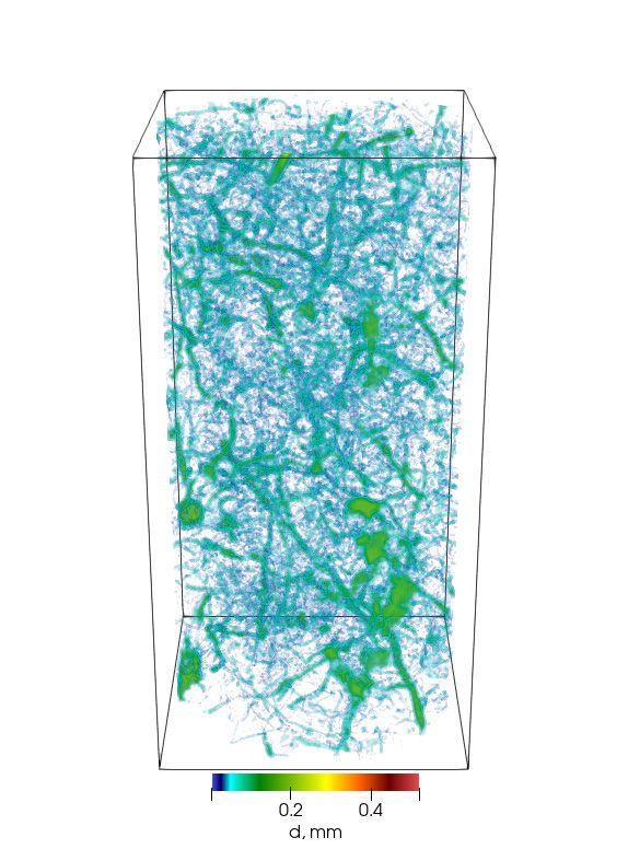
Geosciences 2020, 10, 365 3 of 13
Geosciences 2020, 10, x FOR PEER REVIEW 3 of 13
in the form of truncated cone, where the upper base diameter was congruent to the syringe diameter
syringe
and the diameter
lower base and the lower
diameter was base
2–3diameter
cm widerwasthan 2–3 cmsyringe
the wider diameter.
than the syringe
The formdiameter. The form
of the truncated
of theprovided
cone truncated cone provided
stability and reducedstability andof
the risk reduced the risk
monolithic of monolithic
cracking or breaking.cracking
After or breaking.
preparation
After preparation
procedures, procedures,
the syringe the syringe
was pushed on was pushed onby
the monolith theundercutting
monolith by undercutting
the truncatedthe truncated
cone to the
cone to the cylindrical
cylindrical form everyform 5–10every
cm of5–10 cm of
syringe syringeAfter
moving. moving.
the After the monolith
monolith was fullywas fully immersed
immersed into the
into the syringe,
syringe, the sample thewas
sample was
cut in andcutevened
in andfrom
evenedthe from
bottomtheon
bottom on the periphery
the periphery of theand
of the syringe syringe
was
and was
sealed withsealed withtape.
a sticky a sticky tape.
Thirteen monolithic samples were collected for laboratory laboratory investigation with X-ray computed computed
tomography. Samples
tomography. Sampleswere werecollected
collectedfromfromdifferent
differenthorizons
horizons ofof Phaeozem
Phaeozem albic
albic soil.
soil. AA visualization
visualization of
of voids
voids fromfromall all samples
samples in dry
in dry conditions
conditions cancan be found
be found in Figure
in Figure 1. 1
computedtomography
X-ray computed tomographywas was carried
carried outout
underunder
twotwo different
different saturation
saturation conditions:
conditions: air-
air-dried
driedsaturated
and and saturated
beyondbeyond
the fieldthe field capacity.
capacity. After the After the first
first air-dry air-dry tomography
tomography scanning, the scanning,
sample was the
sample wasbymoistened
moistened supplyingby supplying
excess excess water
water through through
the base the on
standing base standing
several filteron several
papers. filter
The papers.
imbibition
The imbibition
continued for 7 continued for 7permanent
full days with full days with permanent
watering watering
until the until the
water table rosewater
up totable rose
the top up of
base to the
top base ofThen,
specimen. the specimen.
the sample Then,
wasthefreesample
drainedwason free drained
a sandy baseon a sandythe
reaching base reaching
constant the constant
weight without
weight without
evaporation. Then,evaporation.
a 3D image ofThen, a 3D was
the specimen image of the
acquired specimen
through was acquired
microtomography, with through
a time
microtomography,
acquisition of 2–3 h.with
Soil ahumidity
time acquisition of 2–3during
was constant h. Soil imaging.
humidity was constant during imaging.
Void visualization of all samples in dry conditions.
Figure 1. Void
2.2. X-ray Computed Tomography and Image Analysis
2.2. X-ray Computed Tomography and Image Analysis
The tomographic investigation of pore space structure was carried out with a SkyScan 1172
The tomographic investigation of pore space structure was carried out with a SkyScan 1172
(Belgium) microtomographer with different energy settings for dry (100 kV, 100 µA, Al + Cu filter)
(Belgium) microtomographer with different energy settings for dry (100 kV, 100 μA, Al + Cu filter)
and wet (70 kV, 129 µA, Al filter) samples. The X-ray source was a Hamamatsu 100/250 with 10 W
and wet (70 kV, 129 μA, Al filter) samples. The X-ray source was a Hamamatsu 100/250 with 10 W
output. The imaging parameters were chosen so as to minimize costs (the running time of X-ray tunnel
output. The imaging parameters were chosen so as to minimize costs (the running time of X-ray
and CMOS device) of the microtomographer, but to obtain sufficient final image quality. Soil samples
tunnel and CMOS device) of the microtomographer, but to obtain sufficient final image quality. Soil
consisted of several vertical sections which were acquired in one hour.
samples consisted of several vertical sections which were acquired in one hour.
The projections were reconstructed onto a 3D image with the Feldkamp algorithm [36] implemented
The projections were reconstructed onto a 3D image with the Feldkamp algorithm [36]
in NReckon software. Voids visualization of each sample in dry and moisture-saturated conditions are
implemented in NReckon software. Voids visualization of each sample in dry and moisture-saturated
provided in Supplementary Materials (Figures S1–S11). We obtained 3D sample images with 16-bit
conditions are provided in Supplementary Materials (Figures S1–S11). We obtained 3D sample
arrays and a resolution of 8 micrometers in each direction. After median filtering with a 3 by 3 kernel,
images with 16-bit arrays and a resolution of 8 micrometers in each direction. After median filtering
pores were identified via Fiji [37] implementation of minimum cross entropy thresholding method [38],
with a 3 by 3 kernel, pores were identified via Fiji [37] implementation of minimum cross entropy
which showed the most consistent results. We will only consider the visible porosity because the pores
thresholding method [38], which showed the most consistent results. We will only consider the
smaller than several voxels in size are not resolved.
visible porosity because the pores smaller than several voxels in size are not resolved.
Two-dimensional tomographic images of one soil sample are presented in Figure 2. The sample
was acquired in dry and moisture-saturated conditions. The changes in void structure are visible—
some flat cracks are closed, and cylindrical shaped channels have narrowed.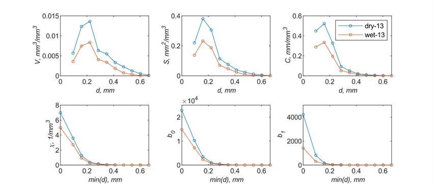
Geosciences 2020, 10, 365                                                                                            4 of 13

       Two-dimensional tomographic images of one soil sample are presented in Figure 2. The sample
was acquired in dry and moisture-saturated conditions. The changes in void structure are visible—some
flat cracks
Geosciences   are10,
            2020, closed,  and cylindrical
                     x FOR PEER REVIEW     shaped channels have narrowed.                        4 of 13

                            (a)                                                           (b)

     Figure
      Figure 2.2. Two-dimensional
                  Two-dimensionalslices
                                      slicesof
                                             oftomographic
                                                tomographicimages
                                                                imagesofofone
                                                                           oneof
                                                                               ofthe
                                                                                  thestudied
                                                                                      studiedsamples
                                                                                                samples(a)
                                                                                                         (a)in
                                                                                                             inaa dry
                                                                                                                  dry
     condition
      condition and
                  and (b) moisture-saturated
                          moisture-saturated condition.
                                                 condition. In
                                                             Inthe
                                                                thetwo
                                                                    twoimages,
                                                                        images,the
                                                                                 thecross
                                                                                     crosssections
                                                                                           sectionscorresponding
                                                                                                     corresponding  to
     to
      thethe same
           same     height
                  height of of
                            thethe specimen
                                 specimen  areare shown.
                                               shown.

3. Minkowski
3. MinkowskiFunctionals
             Functionalsand
                        andBetti
                            BettiNumbers
                                 Numbers

 3.1. Theory
3.1. Theory
      Let X be an object which is bounded by the smooth surface δX in Euclidean d-dimensional
      Let    be an object which is bounded by the smooth surface         in Euclidean d-dimensional
 space. To describe the geometric and topological properties of this object, the integral geometry
space. To describe the geometric and topological properties of this object, the integral geometry
 enables us to determine d + 1 topological invariants that are named Minkowski functionals [39,40].
enables us to determine + 1 topological invariants that are named Minkowski functionals [39,40].
 Here, consideration is given to three-dimensional tomographic images of soil samples. Thus,
Here, consideration is given to three-dimensional tomographic images of soil samples. Thus, only 3-
 only 3-dimensional space will be reviewed. The object of investigation was the pore space because its
dimensional space will be reviewed. The object of investigation was the pore space because its
 structure mainly determines the soil properties. In this case, the Minkowski functionals correspond
structure mainly determines the soil properties. In this case, the Minkowski functionals correspond
 to pores volume, surface area of pores, and integral mean curvature of pore–soil interface and
to pores volume, surface area of pores, and integral mean curvature of pore–soil interface and Euler-
 Euler-Poincare characteristic of pore space:
Poincare characteristic of pore space:
                                                   M0 (X) = V (X), ,                                                     (1)(1)
                                                         Z
                                                       =
                                              M1 ( X ) =    dS== S(X,),                                                  (2)(2)
                                                            δX
                                                     Z            !
                                                          1    1
                                    M2 ( X ) =            1 +1 dS = C(X),                                   (3)
                                             = δX         r1 + r2   =  ,                                  (3)
                                          Z
                                                 1
                                M3 (X) =        11 r2 dS = 2πχ(δX) = 4πχ(X),                                (4)
                                        = δX   r         = 2πχ δ = 4πχ ,                                  (4)
where r1 and r2 are the main radii of surface curvature dS, while χ(δX) and χ(X) are the Euler-Poincare
where      and forarethe
characteristics        thesurface
                           main radii
                                   and of surface
                                       convex        curvature
                                                  body,             , while
                                                          respectively.   To compare andvalues of
                                                                                               areMinkowski
                                                                                                   the Euler-
Poincare   characteristics  for the  surface  and     convex   body,   respectively.  To compare
functionals obtained from different samples, we used normalization. For example, if the size       values   of
                                                                                                        of the
Minkowski
3-dimensionalfunctionals
                image was obtained  from×different
                            1000 × 1000                samples,
                                            1000 voxels,         we values
                                                           then the  used normalization.  For example,
                                                                           of functionals were             109 .
                                                                                                        if the
                                                                                               divided by
size of the 3-dimensional image was 1000 × 1000 × 1000 voxels, then the values of functionals were
divided by 109.
     The Euler-Poincare characteristic for the convex body is an integral estimate of topological
complexity, and can be determined as an alternative summary of Betti numbers:
                                                 =         −          +        ,                                         (5)
Geosciences 2020, 10, 365 5 of 13
The Euler-Poincare characteristic for the convex body is an integral estimate of topological
complexity, and can be determined as an alternative summary of Betti numbers:
χ(X) = b0 (X) − b1 (X) + b2 (X), (5)
where Betti numbers can be interpreted in the context of soil pore space in the following way [31,41]: b0 is
the number of connected components (individual pores), b1 is the number of “tunnels” (or redundant
connections, loops, torus—all types of pores that cannot be compacted into a dot), and b2 is the number
of solid clusters that are completely surrounded by pores (supposed to be equivalent to 1).
Only two phases (pores and solid skeleton) are rationalized in the investigated sample, so,
according to [42,43], Minkowski functionals and Betti numbers were calculated for the pore space.
The water inside the specimens in moisture-saturated condition was not considered. Values for the
solid phase can be determined using an analytic approach.
3.2. Algorithms
The 3-dimensional image of voids can be represented in terms of cubical complexes [44,45].
The additivity of Minkowski functionals affords the use of combinatorial algorithms to calculate them.
There are several algorithms which enable the calculation of Minkowski functional values [40,46,47].
In [46], an algorithm based on calculating the number of different local configurations of 2 × 2 × 2
voxel was proposed, while in [40] an algorithm based on calculating the number of vertices, edges,
faces and voxels in cubical complex was presented:
V (X) = nc , (6)
S(X) = −6nc + 2n f , (7)
2C(X) = 3nc − 2n f + ne , (8)
χ(X) = −nc + n f − ne + nν , (9)
where nc is the number of cubes, n f is the number of faces, ne is the number of edges and nν is the
number of vertices in the cubical complex which is associated with sample voids.
In this study, we used [47] software to compute Minkowski functionals. Zero and second Betti
numbers (numbers of connected clusters of pore space and solid matrix) were calculated using
basic functions of MATLAB [48] and ImageJ [49]. The first Betty number was calculated using the
following equation:
b1 (X) = b0 (X) + b2 (X) − χ(X). (10)
3.3. Mathematical Morphology: Erosion, Dilatation, and Opening Operations
The morphological opening operation used in this study relates to the type of methods which
is called the mathematical morphology. Classical mathematical morphology was proposed in [50],
where the main morphological operations of erosion and dilatation were introduced. Mathematical
morphology was used for tomographic soil images [20,33,51] analysis. A detailed mathematical
morphology methods review describing their applicability for investigations of 2D and 3D images of
natural structures is provided in [52].
The erosion operation leads to object boundaries expansion. Conversely, the dilatation leads to
boundaries narrowing (Figures A1 and A2). An opening operation was obtained by successive usage
of erosion and dilatation operations with structural unit identical form and size for objects:
X ◦ Bd = (X Bd ) ⊕ Bd , (11)
where Bd is the structural spherical shaped unit with diameter d, and symbols and ⊕ define erosion
and dilatation operations, respectively. As a result of the opening operation usage, objects which areGeosciences 2020, 10, 365 6 of 13
smaller than the size of structural unit disappear. Thus, the dependences Mi (d) and bi (d) represents
the cumulative
Geosciences 2020, 10,distribution of Mi and bi over pore sizes. Non-cumulative distributions of Minkowski
x FOR PEER REVIEW 6 of 13
functionals and Betti numbers can be carried out as a derivative of the cumulative distributions.
In Figure
Figure 33 demonstrates
demonstrates the the results
results of
of the
the morphology
morphology opening
opening operation
operation with
with increasing
increasing
structural discus-shaped unit appliance to the sample pore space image.
the sample pore space image. The generation of similar
similar
functionals
functionalsdistributions
distributionsforfor thethe
porepore
spacespace
of samples in dry and
of samples in wet
dry conditions enabled the enabled
and wet conditions quantitative
the
description
quantitativeofdescription
change in of pore spaceinstructure
change duestructure
pore space to soil wetting. Thewetting.
due to soil advantage Theofadvantage
this approach is
of this
that there is no
approach thatneed
theretoisseparate
no needthe pore space
to separate theinto individual
pore space intopore objects [5].
individual pore objects. [5].
Figure 3.
Figure 3. An
Anexample
exampleofofmorphological
morphological opening
opening operation
operation applied
applied withwith structural
structural unitsunits of different
of different sizes
sizes for images of samples from the arable soil horizon. Voids are white and solid phase is
for images of samples from the arable soil horizon. Voids are white and solid phase is black. Each imageblack.
Each image
shows only theshows
pores only thelarger
that are poresthan
that
theare larger unit
structural thansize
theused
structural unit size usedopening.
for the morphological for the
morphological opening.
4. Results and Discussion
4. Results and Discussion
4.1. Topological Analysis of All Samples
4.1. Topological Analysis
The topological of All Samples
invariants (Euler-Poincare characteristic and Betti number) of all samples in
our investigation are reported in Table 1. For samples
The topological invariants (Euler-Poincare from and
characteristic the Betti
arable horizon,
number) ofan
all increase
samples in the
in our
Euler-Poincare characteristic is observed during the wetting process. On the other hand,
investigation are reported in Table 1. For samples from the arable horizon, an increase in the Euler-for samples
from the A2,
Poincare AB, and B2 is
characteristic horizons,
observed theduring
Euler-Poincare characteristic
the wetting process. Ondecreased during
the other hand,wetting (except
for samples for
from
sample 6). All samples were divided into two groups based on mechanism of topological
the A2, AB, and B2 horizons, the Euler-Poincare characteristic decreased during wetting (except for change of
pore
samplespace during
6). All wetting:
samples were divided into two groups based on mechanism of topological change of
pore space
Samples during
with wetting:
a “normal” topology change (samples from 20–90 cm depth, horizons A2, AB, and B2).
Both Betti numbers (number
Samples with a “normal” topology of connected
changeclusters
(samples and number
from 20–90ofcm tunnels)
depth,decreased during
horizons A2, AB,swelling.
and B2).
The Euler-Poincare
Both Betti numberscharacteristic
(numberchange was determined
of connected clusters and by number
the correlation between
of tunnels) closedduring
decreased pores
and closed tunnels:
swelling. In the samplescharacteristic
The Euler-Poincare from the above-mentioned horizons the
change was determined by number of closed
the correlation pores
between
dry dry
closed than
was bigger poresthe
and closed tunnels:
number of closedIntunnels:
the samples
(b0 from wet > babove-mentioned
− b0 the 1
wet horizons the number
− b1 ), so the Euler-Poincare value
decreased. These
of closed samples
pores were taken
was bigger from
than the the horizons
number of closedwhich − agriculturally
had (not been
tunnels: > − exploited,
), so the
so a denser (>1.3 g/cm 3 ) and more stable structure was preserved. Upon wetting, some tunnels are
Euler-Poincare value decreased. These samples were taken from the horizons which had not
closed, or agriculturally
been at least partly exploited,
closed, allowing them(>1.3
so a denser to be subsumed
g/cm3) to the
and more category
stable of individual
structure pores.
was preserved.
In one of the samples taken from 20–30 cm depth from the A2 horizon (sample
Upon wetting, some tunnels are closed, or at least partly closed, allowing them to be subsumed 6), the number of
closedtopores was smaller
the category than the pores.
of individual number Inofone
closed
of thetunnels
samplesandtaken
the Euler-Poincare
from 20–30 cmvaluedepthincreased.
from the
The correlation
A2 horizoncan be explained
(sample 6), the by the individual
number of closedstructural
pores wasfeatures of the
smaller thansamples, particularly
the number of closedby
the large number of small tunnels which closed during wetting (Figure S17).
tunnels and the Euler-Poincare value increased. The correlation can be explained by the
individual structural features of the samples, particularly by the large number of small tunnels
which closed during wetting (Figure S17).
Samples with an “irregular” changing topology (0–20 cm, arable horizon). In these samples, the
(number of tunnels) decreased, but the (number of connected clusters) increased during the
wetting process. In this case, an increase in the number of small pores was observed (this wasGeosciences 2020, 10, 365 7 of 13
Samples with an “irregular” changing topology (0–20 cm, arable horizon). In these samples, the b1
(number of tunnels) decreased, but the b0 (number of connected clusters) increased during the wetting
process. In this case, an increase in the number of small pores was observed (this was also proved by
the increasing integral mean curvature in that range). Apparently, during the swelling, some pores
become smaller but not enough to close. Another explanation can be a mechanism whereby small
pores do not close up because they are filled with an X-ray transparent substance, for example, clamped
pendular water [53]. In samples from the arable horizon at a depth of 10–20 cm, a number of tunnels
narrowed slightly, which can be explained by the presence of plant roots in most tunnels. For the
majority of agricultural crops in a mild climate, about 50% of all plant roots are accumulated at a depth
of 8–20 cm [54]. These roots can keep tunnels open during soil wetting. It should be noted that in one
of the samples from the arable horizon at a depth of 0–10 cm (sample 2), the change in the topology of
the pore space occurred in agreement with the “normal” change (Figure S13).
Table 1. Soil samples used in this study, indicating the occurrence depths and horizons. The three
columns on the right represent the relationship between the Euler-Poincare characteristic and Betti
numbers of the pore space under dry and wet conditions.
dry dry
Sample Depth, cm Horizon Topology χwet vs. χdry bwet
0 vs. b0 bwet
1 vs. b1
1 0–10 Arable Irregular > > <
2 0–10 Arable Normal > < <
3 0–10 Arable Irregular > > <
4 10–20 Arable Irregular > > <
5 10–20 Arable Irregular > > <
6 20–30 A2 Normal > < <
7 20–30 A2 Normal < < <
8 30–40 A2 Normal < < <
9 30–40 A2 Normal < < <
10 40–50 AB Normal < < <
11 40–50 AB Normal - - -
12 80–90 B2 Normal < < <
13 80–90 B2 Normal < < <
4.2. The Detailed Analysis of the Sample from the B2 Horizon
Here, we discuss the pore size distribution of Minkowski functionals and Betti numbers in the
sample from the B2 horizon. The sample was taken from a depth of 80–90 cm and its pore space image
is presented in Figure 4. The dependence graphs for all samples are shown in Supplementary Materials
(Figures S12–S22). The dependencies analysis from Figure 5 suggests that, during soil wetting, the total
sample porosity narrowed across the entire range of pore sizes; furthermore, the specific surface area
of pores narrowed too. The integral mean curvature of pore spaces narrowed by less than 0.4 mm,
which can be explained by the small number of pores closing. These small pores have a large specific
surface curvature. The large pores and tunnels reduced slightly in size and did not change their form,
so their curvature changed minimally.
More detailed changes which take place in the void’s structure are illustrated by the distribution of
the Euler-Poincare characteristic and Betti numbers. The larger the Euler-Poincare value is, the stronger
individual pores dominate over tunnels in a void’s structure. The structures where tunnels prevail
over individual pores have negative values of the Euler-Poincare characteristic.
In a case sample from B2 horizon, a Euler-Poincare characteristic of voids narrows during soil
swelling across the entire range of pore sizes. This means the voids become more bound together
topologically. This can be proved by Betti numbers analysis, which enables visual interpretation.
A zero Betti number is associated with the void’s connected clusters, whereas the first Betti number is
associated with numbers of tunnels in the solid phase. The individual pore spaces (b0 ) are interstices
that do not have exits past the sample boundaries. These pores are closed. The tunnels (b1 ) are openGeosciences 2020, 10, x FOR PEER REVIEW 8 of 13
The distribution analysis suggests that the dry sample contains more individual pores or tunnels
than The distribution
the wet sample, analysis suggests that
with a difference therange
in the dry sample
of 0–0.4contains more individual
mm. Nevertheless, porespores or tunnels
are more likely
than the wet sample, with
to become closed than tunnels: a difference
− in the
> range −of 0–0.4 mm. Nevertheless, pores are more likely
. It is worth noting that the aforementioned
to become closed
correlation is not than tunnels:
universe for all −
samples. > second
The − Betti. Itnumber
is worthequals
noting1that
(it isthe aforementioned
associated with the
Geosciences 2020, 10, 365 8 of 13
correlation is not universe
connected clusters of soils for all samples.
phase which areThe second Betti
surrounded by number
voids) andequals 1 (it
is not is associated
represented with the
in graphs.
connected clusters of soils phase which are surrounded by voids) and is not represented in graphs.
pores with more than one exit past the sample boundaries (perforated pore). It can also be a closed
pore with a form topologically identical to torus.
(a) (b)
(a) (b)
Figure 4. Void visualization of a sample which was taken from 80–90 cm depth from the B2 horizon
Figure
(a) in a4.
Figure Void
4.dryVoid visualization
visualization
condition and (b) of
ofin aa sample
sample which
which was
was taken
a moisture-saturated taken from
from 80–90
condition. The cm
80–90 cm depth
depth from
Euclidean from the
the B2
distance horizon
B2the
to horizon
solid
(a)
(a) in
phasein aais
dry
dry condition
illustrated inand
condition and (b)
color.(b)Itin
in
canaamoisture-saturated
moisture-saturated
be observed that some condition.
condition. The
The Euclidean
small pores Euclidean
and distance
distance
channels to
present the
tointhe solid
solid
the dry
phase
phase is
is illustrated
illustrated in
in color.
color. It
It can
can be
be observed
observed that
that some
some small
small pores
pores and
and channels
channels
sample image on the left are absent from the wet sample image on the right. Large pores and channels present
present in
in the
the dry
dry
sample
sample image
image on
were narrowed the
onbut left
left are
thepresentare absent
absent
in from
from the
the image the wet sample
wetwet
of the sample image
image on
sample. on the
the right.
right. Large
Large pores
pores and
and channels
channels
were narrowed but present in the image of
were narrowed but present in the image of the wet sample. the wet sample.
Figure5.5. Distribution
Figure Distributionof ofpore
porecharacteristics
characteristicsasasa afunction ofof
function pore sizes
pore sizes forfor
a sample from
a sample fromhorizon B2 B2
horizon at
aFigure
atdepth 5.
ofDistribution
a depth 80–90 in aof
cm cm
of 80–90 pore
indry characteristics
condition
a dry (blue
condition ascolor)
a function
color)
(blue andand of pore
wet wet sizes
condition (redfor
condition a color).
sample
color).
(red from
The The
values V, S, C, are
horizon
values ,
B2
at
area depth
represented ofby
80–90
represented bycm in a dry condition
non-cumulative (blue
pores pores
non-cumulative sizes color)
distribution,
sizes andwhereas
distribution, χ, b0 , b1(red
wet condition
whereas , color).
, values
values are The values
presented
are , ,
versus
presented
are
the represented
minimum
versus bydiameter.
pore
the minimum non-cumulative pores
The minimum
pore diameter. sizesdiameter
pore
The minimum distribution, whereas
corresponds
pore diameter , ,diameter
to the
corresponds values
to the ofare
thepresented
spherical
diameter of the
versus the
structural minimum
unit used pore
for diameter.
morphological The minimum
opening.
spherical structural unit used for morphological opening. pore diameter corresponds to the diameter of the
spherical structural unit used for morphological opening.
The distribution analysis suggests that the dry sample contains more individual pores or tunnels
than the wet sample, with a difference in the range of 0–0.4 mm. Nevertheless, pores are more likely
dry dry
to become closed than tunnels: b0 − bwet
0
> b1 − bwet
1
. It is worth noting that the aforementionedGeosciences 2020, 10, 365 9 of 13
correlation is not universe for all samples. The second Betti number equals 1 (it is associated with the
connected clusters of soils phase which are surrounded by voids) and is not represented in graphs.
5. Conclusions
Here we presented the methodological base of the void structure quantitative description.
The methodology is based on the methods from integral geometry, topology, and mathematical
morphology. Methodology can be applied to media with complex internal structures at different scales,
including but not limited to soils, sedimentary rocks, foams, ceramics, and composite materials.
The void structure’s evolution of 13 monolithic samples during soil wetting was quantitatively
illustrated. To quantitatively demonstrate the changes in the structure of the pore space, an analysis of
the evolution of the Minkowski functionals and Betti numbers was carried out. The results suggest
that quantitative topological analysis can be used to describe either the void structure or the changes
in internal structure of voids which are initiated by some external effect or process. We found that
the topology of the void space in the process of soil saturation can change in two ways. A “normal”
change in topology implies a decrease in the zero and first Betty numbers of the pore space, and is
observed in soils from the A2, AB, and B2 horizons at a depth of 20–90 cm. An “irregular” change
in the pore space was found for soils from the arable horizon at a depth of 0–20 cm. The zero Betty
number of the pore space for these samples increased and then decreased during wetting.
Eventually, we plan to transition from quantitative characteristics of pore space to the functional
characteristics of hydro-physical properties of soil. The future target of research is the degraded soils.
The possibility of association of Minkowski functionals and Betti numbers with physical properties
such as field capacity, wilting moisture content, bubbling pressure, hydraulic conductivity, and other
physical pedological characteristics will be investigated.
Supplementary Materials: The following are available online at http://www.mdpi.com/2076-3263/10/9/365/s1,
Figures S1–11: Void visualization of samples taken from different depths and horizons in dry and moisture-saturated
conditions; Figures S12–S22: Distribution of specific pore volumes, surface areas and integral mean curvature of
pore surfaces, Euler-Poincare characteristics and Betti numbers as a function of pore sizes for a samples at different
depths and horizons in dry and moisture-saturated conditions.
Author Contributions: Conceptualization, E.S., D.I.; methodology, T.K., E.S., D.I.; software, D.I.; validation, E.S.,
E.G.; formal analysis, T.K.; investigation, T.K.; resources, T.K., E.S.; data curation, D.I., E.S.; writing—original
draft preparation, D.I.; writing—review and editing, D.I., T.K., E.S.; visualization, D.I.; supervision, E.S., E.G.;
project administration, E.S.; funding acquisition, E.S. All authors have read and agreed to the published version of
the manuscript.
Funding: The work was partly supported by the RFBR, project 19-29-05112_mk, “Digital physics and soil hydrology:
the basics of spatial-dynamic analysis, prediction of risks of critical situations and optimal control”.
Acknowledgments: The authors are grateful to K.N. Abrosimov for help with obtaining tomographic images of
soils. The tomographic work was carried out with the involvement of the equipment from the Center for the
Collective Use of Scientific Equipment “Functions and properties of soils and soil cover” of V.V. Dokuchaev Soil
Science Institute. The authors also thank the three anonymous reviewers, whose insightful comments helped
improve the manuscript.
Conflicts of Interest: The authors declare no conflict of interest.
Appendix A
Table A1. Physical and chemical properties of silty loam Phaeozem albic.
Soil Texture Diameter, mm Sat. Hydraulic
Depth, cm Horizons Density, g/cm3 FC, % vol.
0.05 Conductivity, cm/Days
0–5 17.39 80.66 1.95 1.1 37.3 60
0–10 Arable 17.35 80.21 2.44 1.16 37.2 58
10–20 17.21 80 2.79 1.21 37 52
20–30 17.03 81.62 1.75 1.33 38.6 26
A2
30–40 16 82.43 1.57 1.36 38.2 32Appendix A
Table A1. Physical and chemical properties of silty loam Phaeozem albic.
Table A1. Physical and chemical properties of silty loam Phaeozem albic.
Soil
Soil Texture
Texture Diameter,
Diameter, mm
mm FC,
FC, Sat.
Sat. Hydraulic
Hydraulic
Depth,
Depth, Density,
Density,
Horizons
Horizons %
% Conductivity,
Conductivity,
cm
Geosciences
cm 2020, 10, 365 0.05 g/cm3
g/cm3 10 of 13
vol.
vol. cm/Days
cm/Days
0–5
0–5 17.39
17.39 80.66
80.66 1.95
1.95 1.1
1.1 37.3
37.3 60
60
0–10
0–10 Arable
Arable 17.35
17.35 80.21 2.44
Table A1. Cont.
80.21 2.44 1.16
1.16 37.2
37.2 58
58
10–20
10–20 17.21
17.21 80
80 2.79
2.79 1.21
1.21 37
37 52
52
Soil Texture Diameter, mm Sat. Hydraulic
20–30
Depth,
20–30
cm Horizons 17.03 81.62
0.05
1.75
Density,
1.75 g/cm
3 1.33 38.6
38.6Conductivity,26
FC, % vol.
1.33 26
cm/Days
A2
A2
30–40
30–40 16 82.43 1.57 1.36
1.36 37.4 38.2 32
40–50 17.35 16 81.76 82.430.89 1.57
1.33 38.2 35 32
40–50 AB 17.35 81.76 0.89 1.33
50–60
40–50 AB 17.32 17.35 82.09 81.760.59 1.39
0.89 1.33 35.3 37.4
37.4 35 35
35
50–60 AB 17.32 82.09 0.59 1.39
50–60
80–100 B2 18.4 17.32 81.1 82.090.5 0.591.4 1.39 37.6 35.3
35.3 28.535
35
80–100
80–100 B2
B2 18.4
18.4 81.1
81.1 0.5
0.5 1.4
1.4 37.6
37.6 28.5
28.5
FigureA1.
A1. An example
example of morphological
morphological erosion operation
operationapplied
appliedwith
withstructural
structuralunits
unitsof different
Figure A1.An
Figure An example of
of morphological erosion operation applied with structural units ofofdifferent
different
sizesfor
sizes forimages
imagesof
ofsamples
samples from
from the
the arable
arable soil
soil horizon.
horizon. Voids
Voids are
are white
white and
and solid
solid phase
phase isisblack.
black.
sizes for images of samples from the arable soil horizon. solid phase is black.
Figure A2. An example of morphological dilatation operation applied with structural units of
Figure A2. An example of morphological dilatation operation applied with structural units of
Figure An example
A2.sizes
different of of
for images morphological
samples fromdilatation
the arableoperation applied
soil horizon. with
Voids arestructural
white andunits
solidofphase
different
is
different sizes for images of samples from the arable soil horizon. Voids are white and solid phase is
sizes for
black. images of samples from the arable soil horizon. Voids are white and solid phase is black.
black.
References
1. Zhao, S.; Zhao, Y.; Wu, J. Quantitative analysis of soil pores under natural vegetation successions on the
Loess Plateau. Sci. China Earth Sci. 2010, 53, 617–625. [CrossRef]
2. Costanza-Robinson, M.S.; Estabrook, B.D.; Fouhey, D.F. Representative elementary volume estimation for
porosity, moisture saturation, and air-water interfacial areas in unsaturated porous media: Data quality
implications. Water Resour. Res. 2011, 47. [CrossRef]Geosciences 2020, 10, 365 11 of 13
3. Rigby, S.P.; Chigada, P.I.; Wang, J.; Wilkinson, S.K.; Bateman, H.; Al-Duri, B.; Wood, J.; Bakalis, S.; Miri, T.
Improving the interpretation of mercury porosimetry data using computerised X-ray tomography and
mean-field DFT. Chem. Eng. Sci. 2011, 66, 2328–2339. [CrossRef]
4. Karsanina, M.V.; Gerke, K.M.; Skvortsova, E.B.; Ivanov, A.L.; Mallants, D. Enhancing image resolution of
soils by stochastic multiscale image fusion. Geoderma 2018, 314, 138–145. [CrossRef]
5. Houston, A.N.; Otten, W.; Falconer, R.; Monga, O.; Baveye, P.C.; Hapca, S.M. Quantification of the pore size
distribution of soils: Assessment of existing software using tomographic and synthetic 3D images. Geoderma
2017, 299, 73–82. [CrossRef]
6. Leue, M.; Uteau-Puschmann, D.; Peth, S.; Nellesen, J.; Kodešová, R.; Gerke, H.H. Separation of Soil Macropore
Types in Three-Dimensional X-Ray Computed Tomography Images Based on Pore Geometry Characteristics.
Vadose Zone J. 2019, 18, 1–13. [CrossRef]
7. Armstrong, R.T.; McClure, J.E.; Robins, V.; Liu, Z.; Arns, C.H.; Schlüter, S.; Berg, S. Porous
Media Characterization Using Minkowski Functionals: Theories, Applications and Future Directions.
Transp. Porous Media 2018. [CrossRef]
8. Gregorová, E.; Uhlířová, T.; Pabst, W.; Diblíková, P.; Sedlářová, I. Microstructure characterization of mullite
foam by image analysis, mercury porosimetry and X-ray computed microtomography. Ceram. Int. 2018, 44,
12315–12328. [CrossRef]
9. Pabst, W.; Uhlířová, T.; Gregorová, E. Microstructure Characterization of Porous Ceramics Via Minkowski
Functionals. In Ceramic Transactions Series; Singh, D., Fukushima, M., Kim, Y.-W., Shimamura, K., Imanaka, N.,
Ohji, T., Amoroso, J., Lanagan, M., Eds.; John Wiley & Sons, Inc.: Hoboken, NJ, USA, 2018; pp. 53–64.
ISBN 978-1-119-49409-6.
10. Tsukanov, A.; Ivonin, D.; Gotman, I.; Gutmanas, E.Y.; Grachev, E.; Pervikov, A.; Lerner, M. Lerner Effect of
Cold-Sintering Parameters on Structure, Density, and Topology of Fe–Cu Nanocomposites. Materials 2020,
13, 541. [CrossRef] [PubMed]
11. Mecke, K.R.; Wagner, H. Euler characteristic and related measures for random geometric sets. J Stat. Phys.
1991, 64, 843–850. [CrossRef]
12. Arns, C.H.; Knackstedt, M.A.; Mecke, K.R. Characterisation of irregular spatial structures by parallel sets
and integral geometric measures. Colloids Surf. A Physicochem. Eng. Asp. 2004, 241, 351–372. [CrossRef]
13. Arns, C.; Knackstedt, M.; Martys, N. Cross-property correlations and permeability estimation in sandstone.
Phys. Rev. E 2005, 72, 046304. [CrossRef] [PubMed]
14. Feng, Y.; Wang, J.; Liu, T.; Bai, Z.; Reading, L. Using computed tomography images to characterize the effects
of soil compaction resulting from large machinery on three-dimensional pore characteristics in an opencast
coal mine dump. J. Soils Sediments 2019, 19, 1467–1478. [CrossRef]
15. San José Martínez, F.; Martín, L.; García-Gutiérrez, C. Minkowski Functionals of Connected Soil Porosity as
Indicators of Soil Tillage and Depth. Front. Environ. Sci. 2018, 6, 55. [CrossRef]
16. San José Martínez, F.; Muñoz Ortega, F.J.; Caniego Monreal, F.J.; Kravchenko, A.N.; Wang, W. Soil aggregate
geometry: Measurements and morphology. Geoderma 2015, 237–238, 36–48. [CrossRef]
17. Çeçen, A.; Wargo, E.A.; Hanna, A.C.; Turner, D.M.; Kalidindi, S.R.; Kumbur, E.C. 3-D Microstructure Analysis
of Fuel Cell Materials: Spatial Distributions of Tortuosity, Void Size and Diffusivity. J. Electrochem. Soc. 2012,
159, B299–B307. [CrossRef]
18. Wyss, P.; Flisch, A.; Lehmann, E.; Vontobel, P.; Krafczyk, M.; Kaestner, A.; Beckmann, F.; Gygi, A.; Flühler, H.
Tomographical Imaging and Mathematical Description of Porous Media Used for the Prediction of Fluid
Distribution. Vadose Zone J. 2006, 5. [CrossRef]
19. Wang, W.; Kravchenko, A.N.; Smucker, A.J.M.; Liang, W.; Rivers, M.L. Intra-aggregate Pore Characteristics:
X-ray Computed Microtomography Analysis. Soil Sci. Soc. Am. J. 2012, 76, 1159–1171. [CrossRef]
20. San José Martínez, F.; Muñoz-Ortega, F.; Caniego, J.; Peregrina, F. Morphological Functions to Quantify
Three-Dimensional Tomograms of Macropore Structure in a Vineyard Soil with Two Different Management
Regimes. Vadose Zone J. 2013, 12. [CrossRef]
21. Berg, C.F. Permeability Description by Characteristic Length, Tortuosity, Constriction and Porosity.
Transp. Porous Media 2014, 103, 381–400. [CrossRef]
22. Akai, T.; Lin, Q.; Alhosani, A.; Bijeljic, B.; Blunt, M. Quantification of Uncertainty and Best Practice in
Computing Interfacial Curvature from Complex Pore Space Images. Materials 2019, 12, 2138. [CrossRef]Geosciences 2020, 10, 365 12 of 13
23. McClure, J.E.; Armstrong, R.T.; Berrill, M.A.; Schlüter, S.; Berg, S.; Gray, W.G.; Miller, C.T. A geometric state
function for two-fluid flow in porous media. Phys. Rev. Fluids 2018, 3, 084306. [CrossRef]
24. Vogel, H.-J. Topological Characterization of Porous Media. In Morphology of Condensed Matter; Mecke, K.,
Stoyan, D., Eds.; Springer: Berlin/Heidelberg, Germany, 2002; Volume 600, pp. 75–92, ISBN 978-3-540-44203-5.
25. Falconer, R.E.; Houston, A.N.; Otten, W.; Baveye, P.C. Emergent Behavior of Soil Fungal Dynamics: Influence
of Soil Architecture and Water Distribution. Soil Sci. 2012, 177, 111–119. [CrossRef]
26. Khachkova, T.S.; Bazaikin, Y.V.; Lisitsa, V.V. Use of the computational topology to analyze the pore space
changes during chemical dissolution. Numer. Methods Program. 2020, 21, 41–55. [CrossRef]
27. Diel, J.; Vogel, H.-J.; Schlüter, S. Impact of wetting and drying cycles on soil structure dynamics. Geoderma
2019, 345, 63–71. [CrossRef]
28. Weller, U.; Leuther, F.; Schlüter, S.; Vogel, H.-J. Quantitative Analysis of Water Infiltration in Soil Cores Using
X-Ray. Vadose Zone J. 2018, 17. [CrossRef]
29. Pires, L.F.; Auler, A.C.; Roque, W.L.; Mooney, S.J. X-ray microtomography analysis of soil pore structure
dynamics under wetting and drying cycles. Geoderma 2020, 362, 114103. [CrossRef] [PubMed]
30. Vogel, H.-J.; Roth, K. Quantitative morphology and network representation of soil pore structure.
Adv. Water Resour. 2001, 24, 233–242. [CrossRef]
31. Vogel, H.J. Morphological determination of pore connectivity as a function of pore size using serial sections.
Eur. J. Soil Sci. 1997, 48, 365–377. [CrossRef]
32. Vogel, H.J.; Kretzschmar, A. Topological characterization of pore space in soil—Sample preparation and
digital image-processing. Geoderma 1996, 73, 23–38. [CrossRef]
33. Vogel, H.-J.; Weller, U.; Schlüter, S. Quantification of soil structure based on Minkowski functions.
Comput. Geosci. 2010, 36, 1236–1245. [CrossRef]
34. Shein, E.V.; Troshina, O.A. Physical properties of soils and the simulation of the hydrothermal regime for the
complex soil cover of the Vladimir Opol’e region. Eurasian Soil Sci. 2012, 45, 968–976. [CrossRef]
35. Shein, E.V.; Kiryushin, V.I.; Korchagin, A.A.; Mazirov, M.A.; Dembovetskii, A.V.; Il’in, L.I. Assessment of
agronomic homogeneity and compatibility of soils in the Vladimir Opolie region. Eurasian Soil Sci. 2017, 50,
1166–1172. [CrossRef]
36. Feldkamp, L.A.; Davis, L.C.; Kress, J.W. Practical cone-beam algorithm. J. Opt. Soc. Am. 1984, 1, 612–619.
[CrossRef]
37. Schindelin, J.; Arganda-Carreras, I.; Frise, E.; Kaynig, V.; Longair, M.; Pietzsch, T.; Preibisch, S.; Rueden, C.;
Saalfeld, S.; Schmid, B.; et al. Fiji: An open-source platform for biological-image analysis. Nat. Methods 2012,
9, 676–682. [CrossRef]
38. Li, C.H.; Lee, C.K. Minimum cross entropy thresholding. Pattern Recognit. 1993, 26, 617–625. [CrossRef]
39. Hadwiger, H. Vorlesungen Über Inhalt, Oberfläche und Isoperimetrie; Springer: Berlin/Heidelberg, Germany, 1957.
40. Michielsen, K.; De Raedt, H. Integral-geometry morphological image analysis. Phys. Rep. 2001, 347, 461–538.
[CrossRef]
41. Bazaikin, Y.; Gurevich, B.; Iglauer, S.; Khachkova, T.; Kolyukhin, D.; Lebedev, M.; Lisitsa, V.; Reshetova, G.
Effect of CT image size and resolution on the accuracy of rock property estimates: EFFECT OF CT IMAGE
SCALE. J. Geophys. Res. Solid Earth 2017, 122, 3635–3647. [CrossRef]
42. Rabot, E.; Wiesmeier, M.; Schlüter, S.; Vogel, H.-J. Soil structure as an indicator of soil functions: A review.
Geoderma 2018, 314, 122–137. [CrossRef]
43. Baveye, P.C.; Otten, W.; Kravchenko, A.; Balseiro-Romero, M.; Beckers, É.; Chalhoub, M.; Darnault, C.;
Eickhorst, T.; Garnier, P.; Hapca, S.; et al. Emergent Properties of Microbial Activity in Heterogeneous Soil
Microenvironments: Different Research Approaches Are Slowly Converging, Yet Major Challenges Remain.
Front. Microbiol. 2018, 9. [CrossRef]
44. Werman, M.; Wright, M.L. Intrinsic Volumes of Random Cubical Complexes. Discret. Comput. Geom. 2016,
56, 93–113. [CrossRef]
45. Kaczynski, T.; Mischaikow, K.; Mrozek, M. Computational Homology; Applied Mathematical Sciences;
Springer-Verlag: New York, NY, USA, 2004; ISBN 978-0-387-40853-8.
46. Schladitz, K.; Ohser, J.; Nagel, W. Measuring Intrinsic Volumes in Digital 3d Images. In Discrete Geometry
for Computer Imagery; Kuba, A., Nyúl, L.G., Palágyi, K., Eds.; Springer: Berlin/Heidelberg, Germany, 2006;
Volume 4245, pp. 247–258, ISBN 978-3-540-47651-1.Geosciences 2020, 10, 365 13 of 13
47. Legland, D.; Kiêu, K.; Devaux, M.-F. Computation of Minkowski measures on 2D and 3D binary images.
Image Anal. Stereol. 2011, 26, 83. [CrossRef]
48. 3-D Volumetric Image Processing—MATLAB & Simulink. Available online: https://www.mathworks.com/
help/images/3d-volumetric-image-processing.html?s_tid=CRUX_lftnav (accessed on 18 August 2020).
49. Schindelin, J.; Rueden, C.T.; Hiner, M.C.; Eliceiri, K.W. The ImageJ ecosystem: An open platform for
biomedical image analysis. Mol. Reprod. Dev. 2015, 82, 518–529. [CrossRef] [PubMed]
50. Serra, J. Image Analysis and Mathematical Morphology; Academic Press, Inc.: Orlando, FL, USA, 1983;
ISBN 978-0-12-637240-3.
51. San José Martínez, F.; Muñoz-Ortega, F.; Caniego, J.; Peregrina, F. Morphological Functions with Parallel Sets
for the Pore Space of X-ray CT Images of Soil Columns. Pure Appl. Geophys. 2014. [CrossRef]
52. Ohser, J.; Schladitz, K. 3D Images of Materials Structures: Processing and Analysis; Wiley-VCH Verlag GmbH &
Co. KGaA: Weinheim, Germany, 2009; ISBN 978-3-527-62830-8.
53. Faybishenko, B.A. Hydraulic Behavior of Quasi-Saturated Soils in the Presence of Entrapped Air: Laboratory
Experiments. Water Resour. Res. 1995, 31, 2421–2435. [CrossRef]
54. Fan, J.; McConkey, B.; Wang, H.; Janzen, H. Root distribution by depth for temperate agricultural crops.
Field Crop. Res. 2016, 189, 68–74. [CrossRef]
© 2020 by the authors. Licensee MDPI, Basel, Switzerland. This article is an open access
article distributed under the terms and conditions of the Creative Commons Attribution
(CC BY) license (http://creativecommons.org/licenses/by/4.0/).You can also read