Can astrophysical neutrinos trace the origin of the detected ultra-high energy cosmic rays? - desy pubdb
←
→
Page content transcription
If your browser does not render page correctly, please read the page content below
MNRAS 494, 4255–4265 (2020)                                                                                                doi:10.1093/mnras/staa1003
Advance Access publication 2020 April 15

Can astrophysical neutrinos trace the origin of the detected ultra-high
energy cosmic rays?

Andrea Palladino,‹ Arjen van Vliet, Walter Winter and Anna Franckowiak
DESY, Platanenallee 6, D-15738 Zeuthen, Germany

                                                                                                                                                          Downloaded from https://academic.oup.com/mnras/article/494/3/4255/5820235 by DESY-Zentralbibliothek user on 10 September 2020
Accepted 2020 April 2. Received 2020 March 30; in original form 2019 November 19

                                       ABSTRACT
                                       Since astrophysical neutrinos are produced in the interactions of cosmic rays, identifying the
                                       origin of cosmic rays using directional correlations with neutrinos is one of the most interesting
                                       possibilities of the field. For that purpose, especially the Ultra-High Energy Cosmic Rays
                                       (UHECRs) are promising, as they are deflected less by extragalactic and Galactic magnetic
                                       fields than cosmic rays at lower energies. However, photo-hadronic interactions of the UHECRs
                                       limit their horizon, while neutrinos do not interact over cosmological distances. We study the
                                       possibility to search for anisotropies by investigating neutrino-UHECR correlations from the
                                       theoretical perspective, taking into account the UHECR horizon, magnetic-field deflections,
                                       and the cosmological source evolution. Under the assumption that the neutrinos and UHECRs
                                       all come from the same source class, we demonstrate that the non-observation of neutrino
                                       multiplets strongly constrains the possibility to find neutrino-UHECR correlations.
                                       Key words: neutrinos – cosmic rays – diffuse radiation.

                                                                               distance. This analysis uses a high-purity but low-statistic sample
1 I N T RO D U C T I O N
                                                                               of IceCube events, focused on energies above 60 TeV. Secondly,
The first hints for the sources of Ultra-High Energy Cosmic Rays               using the same neutrino sample as the first analysis, a stacking
(UHECRs) have been observed, as correlations with catalogues of                of the neutrino arrival directions has been applied, searching for
starburst galaxies and Active Galactic Nuclei (AGNs) reach the                 coincident sources of cosmic rays. The cosmic ray arrival direction
∼4σ level (Aab et al. 2018; Caccianiga et al. 2019). However, a                has been smeared by the observatories’ angular uncertainties and an
definitive answer to the question of the origin of UHECRs remains              energy-dependent Galactic magnetic deflection based on a Galactic
illusive. Moreover, the discovery of a diffuse flux of high energy             Magnetic Field (GMF) model. The third analysis has used a high-
neutrinos by IceCube in 2013 (Aartsen et al. 2013) has opened                  statistics, but low-purity neutrino data sample of both IceCube and
new possibilities to search for the sources of UHECRs. Indeed,                 ANTARES events in the energy range from 1 TeV to 1 PeV, which
it is commonly believed that sources that are able to accelerate               was optimized for the search of neutrino point sources. A search
protons up to very high energies are also good neutrino-emitter                for neutrino point sources in the vicinity of the UHECR arrival
candidates. The knowledge of the cosmic ray flux and the connection            directions has been performed using a stacking analysis. This is
expected between these two astrophysical messengers have already               essentially a point-source stacking analysis with a spatial prior given
been discussed more than 50 yr ago (Berezinsky & Zatsepin 1969).               by the UHECR’s direction uncertainty, smeared with an energy-
In the work presented here we investigate the probability to observe           dependent Galactic magnetic deflection. No significant excess has
spatial correlations between high energy neutrinos and cosmic rays,            been found in any of the three analyses. These non-detections of
assuming that they are produced by the same source class.                      correlations suggest to analyse the problem from a theoretical point
   Three different experimental searches for a correlation of high             of view, in order to understand if there are conditions in which
energy cosmic rays and neutrinos have been performed (Aartsen                  correlations are likely to be observed.
et al. 2016; Schumacher et al. 2019). All three analyses use an                   It is important to recall that neutrinos and cosmic rays propagate
UHECR sample consisting of events above 52 EeV and 57 EeV                      in a very different manner. While this is clear immediately from
recorded by the Pierre Auger Observatory and Telescope Array                   the basic properties of the particles, it will turn out to be one of the
(TA) experiments, respectively. First, a cross-correlation analysis            main reasons which will prevent us from observing correlations –
has counted the number of neutrino-UHECR pairs separated by                    and which we are going to quantify in this work. While neutrinos
less than a given angular distance. This number has been compared              propagate on geodesics, cosmic rays are strongly deflected by both
to the simulated number of random pairs within the same angular                extragalactic and Galactic magnetic fields. Moreover, astrophysical
                                                                               neutrinos lose energy only due to the adiabatic expansion of the
                                                                               Universe, while UHECRs, depending on energy and composition,
   E-mail: andrea.palladino@desy.de                                           lose energy due to adiabatic expansion, Bethe Heitler pair produc-


C 2020 The Author(s)

Published by Oxford University Press on behalf of the Royal Astronomical Society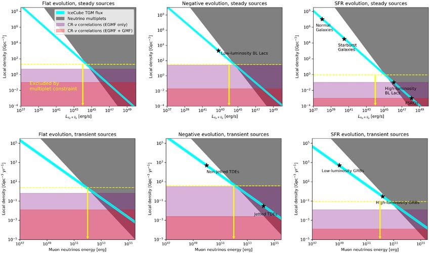
4256         A. Palladino et al.
tion, photo-meson production and photodisintegration on cosmic                    of Fig. 1 we show the contribution to the neutrino luminosity as a
background light. As a consequence, UHECRs can only reach the                     function of redshift. This function fν (z) is proportional to
Earth when they are produced in the local Universe. On the contrary,                                dVc
astrophysical neutrinos can reach the Earth over cosmological                     fν (z) ∝ ρ(z) ×       × D (z)−2 ,                                       (1)
                                                                                                     dz
distances – which implies that the source evolution of the source
class plays a crucial role in our study. We will use three differ-                where dV dz
                                                                                             c
                                                                                               is the comoving volume and D (z) is the luminosity
ent examples characterizing different classes of sources: negative                         2
                                                                                  distance (both functions are defined in Appendix A). We assume
source evolution (which may characterize Tidal Disruption Events                  that sources are standard candles, which means that no source-
(TDEs) Sun, Zhang & Li 2015 or low-luminosity blazars Ajello et al.               luminosity dependence is contained in the previous expression. Let

                                                                                                                                                                  Downloaded from https://academic.oup.com/mnras/article/494/3/4255/5820235 by DESY-Zentralbibliothek user on 10 September 2020
2014), flat evolution (which is the simplest assumption of a source               us recall that neutrinos are not deflected during the propagation and
class present independent of redshift), and Star Formation Rate                   they are only affected by adiabatic energy losses.
(SFR) evolution (Yuksel et al. 2008) (which roughly describes most
conventional source classes, including normal galaxies, starburst
galaxies, high luminosity BL Lacs, Flat Spectrum Radio Quasars                    2.2 Cosmic rays
(FSRQs), and Gamma-Ray Bursts (GRBs)).                                            The case of UHECRs is more complex than the neutrino case. Due
   In this study, we scrutinize the hypothesis that a common origin               to the additional energy-loss processes on the way, very energetic
of the astrophysical neutrinos and UHECRs can be identified from                  cosmic rays can only come from the local Universe, while neutrinos
directional correlations, assuming that both UHECRs and neutrinos                 can reach the Earth from distant sources as well. In addition, cosmic
stem from the same source class. We will define a model using a                   rays are deflected during the propagation by both extragalactic and
Monte Carlo simulation, based on simple counting statistics, and                  Galactic magnetic fields.
we will quantify the impact of magnetic-field deflections, cosmic                    To take into account these effects we compute the spectrum and
source evolution, and particle interactions during propagation.                   composition of UHECRs using CRPropa 3 (Alves Batista et al.
Using the same methods, we will also point out that the obser-                    2016) in the 1D mode. For each source-evolution scenario values
vation of neutrino-UHECR correlations implies the observation of                  for the spectral index (γ ), maximum rigidity (Rmax ) and composition
neutrino multiplets. With the term multiplet we mean two or more                  (specified by proton (fp ), helium (fHe ), nitrogen (fN ) and silicon (fSi )
tracks above 200 TeV (the threshold of the throughgoing muon                      fractions) at the sources are obtained that provide good fits to both
sample) coming from the same direction, within the typical angular                the measured spectrum and composition of UHECRs by Auger,
resolution of track-like events (i.e. 1◦ ) and within the lifetime of             assuming an injected source spectrum of
the IceCube experiment.1 Our purpose is to identify the remaining                          ⎧
parameter space where a common neutrino-UHECR origin can be                       dNi      ⎨fi E −γ                          for E < Zi Rmax ,
identified.                                                                             ∝
                                                                                   dE      ⎩fi E −γ exp 1 − E                for E ≥ Zi Rmax ,
                                                                                                                 Zi Rmax

2 METHOD                                                                          with E and Zi the cosmic ray energy and charge at the source,
                                                                                  respectively. For the negative source evolution case the best-fitting
In a nutshell, we use a Monte Carlo simulation to extract a                       values were taken from Aab et al. (2017), for the flat and SFR
number of sources randomly distributed in the sky, following a                    source evolution they were taken from Alves Batista et al. (2019).
given redshift distribution, assuming that these sources are the                  In all three cases the same UHECR data set as measured by
common sources of neutrinos and UHECRs. Then we propagate                         Auger was used in the fits, for details see Aab et al. (2017).
both neutrinos and cosmic rays, taking into account the energy                    These three fits all assumed EPOS LHC as hadronic interaction
loss of neutrinos and cosmic rays as well as the deflection of                    model in UHECR air showers and the full Xmax distributions,
cosmic rays. Our simulated rates are chosen to match observations                 including their associated errors, were fitted for each energy bin.
provided by Auger and IceCube by taking into account the number                   See Table 1 for the best-fitting values that were found in Aab
of events detected by the two experiments. Finally, we compute the                et al. (2017) and Alves Batista et al. (2019) and are used in this
probability to discriminate a 5σ signal (i.e. cosmic ray events within            work.
a certain angular distance from neutrino events) from a background                   For these three scenarios the contribution to the UHECR flux as
consisting of isotropically distributed events.                                   a function of the redshift has been obtained for cosmic ray energies
                                                                                  at Earth of ECR > 1018.5 eV, see Fig. 1 lower right-hand panel.
                                                                                  Due to the different energy-loss processes the UHECRs can only
2.1 Neutrinos
                                                                                  arrive from relatively nearby sources. The redshift dependence of
First of all, we define three different source evolutions (ρ(z)), as a            the contribution to the UHECR flux is, therefore, quite similar for
function of redshift (z): (i) a negative source evolution, following              the three different source-evolution scenarios considered here, and
an (1 + z)−3 behaviour as a function of redshift; (ii) a flat source              is very different from the neutrino case (Fig. 1 upper right-hand
evolution; (iii) SFR evolution. These source evolutions are shown                 panel).
in the upper left-hand panel of Fig. 1. Other details concerning the                 The expected deflections of cosmic rays due to Extragalactic
source evolutions and the definition of the required cosmological                 Magnetic Fields (EGMFs) (EGMF (z)) as a function of the redshift
functions are reported in Appendix A. In the upper right-hand panel               for ECR > 1018.5 eV have been computed in a 3D simulation

1 Inprinciple, it is also possible to use a lower energy threshold, but in this   2 Note that in that equation it is implicitly assumed that the neutrino flux
case it is hard to discriminate the signal from the background. Moreover,         is characterized by a power-law spectrum, at least in the energy region in
neutrino multiplets have already been observed below ∼100 TeV, as in the          which the detector is sensitive. The consequences of a different scenario are
neutrino flare from TXS 0506+056 during 2014–15 (Aartsen et al. 2018).            discussed in Section 4.

MNRAS 494, 4255–4265 (2020)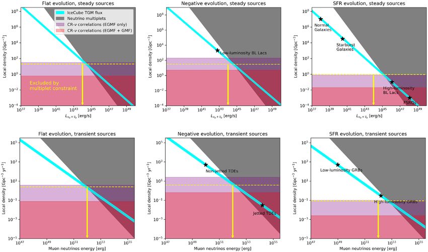
ultra-high energy cosmic rayswith UHECRs                                   4257

                                                                                                                                                                       Downloaded from https://academic.oup.com/mnras/article/494/3/4255/5820235 by DESY-Zentralbibliothek user on 10 September 2020
Figure 1. Upper left-hand panel: the source density as a function of redshift, for three different cases: negative evolution (blue, dashed), flat evolution (orange,
dotted) and sources following the SFR (green, solid). Upper right-hand panel: the corresponding contribution to the neutrino flux as a function of redshift for
the three different source evolution scenarios, considering a power-law spectrum. Lower left-hand panel: the median deflection of cosmic rays for all UHECRs
with ECR > 1018.5 eV, as a function of redshift. Lower right-hand panel: the corresponding contribution to the cosmic ray flux as a function of redshift.

   Table 1. Best-fitting parameters, obtained from Aab et al. (2017)                 EGMFs. The inclusion of adiabatic energy losses would, however,
   and Alves Batista et al. (2019), used in this work for the UHECR                  only have a small effect on EGMF (z) for large redshifts, which are
   simulations.                                                                      not relevant for the expected neutrino-UHECR correlations. The
                                                                                     resulting average deflections as a function of redshift (EGMF (z))
   ρ(z)       γ      Rmax /V        fp        fHe         fN         fSi             are given in Fig. 1 lower left-hand panel. Here EGMF (z) is largest
   Neg.      1.42     1018.85    0.07       0.34        0.53       0.06              in the negative evolution scenario due to the heavier composition at
   Flat    − 1.0      1018.2     0.6726     0.3135      0.0133     0.0006            the sources in that scenario.
   SFR     − 1.3      1018.2     0.1628     0.8046      0.0309     0.0018               Besides the deflections in EGMFs the cosmic rays will also
                                                                                     be deflected in the GMF. To estimate the GMF deflections we
                                                                                     used the distribution of deflections as a function of the rigidity
with CRPropa in a structured EGMF of Hackstein et al. (2018),                        (R) as parametrized by Farrar & Sutherland (2019), taking into
implementing the same best-fitting parameters for the three source-                  account deflections from different directions all over the sky. This
evolution scenarios (Table 1) as well as a continuous distribution                   distribution is parametrized in terms of the mean deflection of
of identical sources. From the six EGMF models described in                          arrival directions (GMF (R)) and the RMS arrival direction spread
Hackstein et al. (2018), we use the ‘astrophysical model’. This                      (σ (GMF )(R)) for the JF12 GMF model (Jansson & Farrar 2012a,
model has the smallest filling factors (fraction of the total space                  b), with Lcoh = 100 pc and Lcoh = 30 pc as correlation lengths for
filled with magnetic fields of a certain strength or stronger) for the               the random component of the GMF. The overall best-fitting values
strongest magnetic fields of the six different modes. This means that                for the parameters of these deflection distributions, as a function of
it can be expected to give the smallest average deflection, leading                  R, are given there by
to a rather conservative estimate for the deflections of UHECRs in
EGMFs. Reflective boundary conditions were implemented in the                               GMF                            R
                                                                                     log10            = (−0.65 ± 0.03) log10     + (13.63 ± 0.59),
simulations to properly include sources at large distances. Adiabatic                         deg                             V
energy losses have not been included in these simulations as, in
                                                                                            σ (GMF )                          R
3D simulations, the total traveltime (redshift) of the particle is                   log10             = (−1.17 ± 0.04) log10     + (23.22 ± 0.71)
not known at the start of the simulation due to the deflections in                             deg                             V

                                                                                                                             MNRAS 494, 4255–4265 (2020)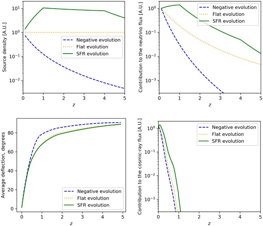
4258           A. Palladino et al.

                                                                                                                                                               Downloaded from https://academic.oup.com/mnras/article/494/3/4255/5820235 by DESY-Zentralbibliothek user on 10 September 2020
Figure 2. Distribution of deflections in the GMF for all UHECRs with ECR > 1018.5 eV and for the three different source evolution scenarios: negative
evolution (blue, dashed), flat evolution (orange, dotted), and sources following the SFR (green, solid). Left-hand panel: the coherence length of the random
component of the GMF Lcoh = 100 pc. Right-hand panel: Lcoh = 30 pc. The results have been normalized so that the area under all curves is equal to one.

for Lcoh = 100 pc and                                                            random and they do not reflect the positions of through-going muons
                                                                             detected by IceCube. We extract 135k UHECRs having E>1018.5 eV
        GMF                            R
log10             = (−0.73 ± 0.04) log10     + (15.23 ± 0.70),                   (roughly the number of cosmic rays in the combined spectrum
          deg                             V                                      detected by Auger for E >1018.5 eV; Fenu et al. 2018). Moreover
                                                                             we are not using the true positions in which cosmic rays and high
        σ (GMF )                          R
log10              = (−1.03 ± 0.03) log10     + (20.30 ± 0.64)                   energy neutrinos have been detected, but both neutrinos and cosmic
           deg                             V
                                                                                 rays are chosen at random locations, as subset of the Ns sources.
for Lcoh = 30 pc. Each particle arriving at Earth in the 1D CRPropa              Therefore cosmic rays and neutrinos have different positions in each
simulations, which were also used to obtain the contribution to                  simulations.
the UHECR flux as a function of the redshift (Fig. 1 lower right-                   (iv) We include that neutrinos follow a straight path, while cosmic
hand panel), is assigned a certain deflection randomly following the             rays are deflected in EGMFs according to the function EGMF (z). In
deflection distribution for its specific rigidity as parametrized by             the lower left-hand panel of Fig. 1 EGMF (z) is illustrated. In the
these equations. In this way a full distribution of GMF deflections              analysis the full distribution of EGMF (z) is used, which has a large
for sources all over the sky is obtained based on the JF12 GMF                   spread (comparable with the median value) not represented in Fig. 1.
model for each specific source-evolution scenario. The resulting                 Additionally, the cosmic rays are deflected in the GMF following
distributions of GMF deflections are given in Fig. 2.                            the distributions given in Fig. 2. We implement here the distribution
                                                                                 for Lcoh = 100 pc as this choice gives the smallest deflections on
                                                                                 average and is, therefore, expected to give the most correlations.
2.3 Monte Carlo simulation
                                                                                    (v) We count the number of cosmic rays within a certain angular
Our Monte Carlo simulation, that is necessary to evaluate under                  distance from the neutrino position. Performing a parameter scan
which conditions we expect correlations between high energy                      we find that the ideal angular window is 5◦ assuming the presence of
neutrinos and UHECRs, is based on the following steps:                           EGMFs only, while this window is much larger (close to 20◦ −30◦ )
                                                                                 when also the GMF is included (see Appendix C for details about
   (i) We extract a number of sources Ns isotropically distributed
                                                                                 this parameter scan). The number of cosmic rays within the angular
in the sky, according to the source evolutions shown in the upper
                                                                                 window represents the sum of signal and background (s + b). Then
left-hand panel of Fig. 1.
                                                                                 we count the average number of cosmic rays within the same angular
   (ii) We assign the probability to observe a neutrino from a certain
                                                                                 window from random positions, which represents the background
source proportional to fν (z) (see upper right-hand panel of Fig. 1),
                                                                                 (b).
while we determine the probability to observe a cosmic ray based
                                                                                    (vi) We sum the number of cosmic rays detected in all angular
on its distribution fCR (z) (see lower right-hand panel of Fig. 1).
                                                                                 windows, and we compare this number with the total number of
   (iii) We extract 36 neutrinos, corresponding to the number of
                                                                                 cosmic rays expected in the same angular windows in case of an
observed through-going muons (Haack et al. 2017), which are the
                                                                                 isotropic distribution. Using the Poissonian likelihood
neutrino events characterized by a good directional resolution of
roughly 1◦ and an energy threshold of 200 TeV, to avoid most of                  χ 2 = 2(b + s) ln(1 + s/b) − 2s,
the atmospheric background.3 The positions of these neutrinos are
                                                                                 we consider that the correlations between neutrinos and UHECRs
                                                                                 can be discovered if χ 2 > 25 (corresponding to 5σ ).
3 Concerning                                                                       (vii) We repeat the entire process 103 times for a given set
               neutrinos, we are implicitly assuming that all the 36 through-
going muons detected by IceCube are of extragalactic origin, neglecting the
                                                                                 of number of sources and source evolutions. At the end of the
possible atmospheric background. This hypothesis maximizes the expected          process roughly 106 sky maps are considered. For each number of
number of correlations between neutrinos and UHECRs. If the atmospheric          sources and each source evolution, we compute how many maps
background is present (or the Galactic plane region is excluded) the             among the 103 maps show significant correlations (according to the
possibility to observe correlations gets worse.                                  definition given above), tagging the map as significant if the excess

MNRAS 494, 4255–4265 (2020)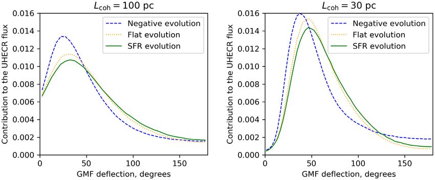
ultra-high energy cosmic rayswith UHECRs 4259
Downloaded from https://academic.oup.com/mnras/article/494/3/4255/5820235 by DESY-Zentralbibliothek user on 10 September 2020
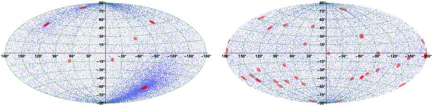
Figure 3. Two different sky maps, in which neutrinos are represented with red discs (for an exaggerated uncertainty of 3◦ , much larger than the typical 1◦
angular uncertainty for tracks) and cosmic rays are represented with blue points. In each sky map 36 neutrinos are shown (the number of neutrinos in the
current IceCube through-going muon sample; Haack et al. 2017), picked at random from Ns sources, together with 105 cosmic ray arrival directions randomly
selected from the same Ns sources. We assume a negative source evolution, ECR ≥ 1019 eV and ρ 0 = 0.1 and 100 Gpc−3 yr−1 for the left-hand and right-hand
panel respectively (corresponding to 8 and 8500 sources). Note that the left sky map shows less than 36 discs because in this case multiple neutrinos arrive
from the same sources. Furthermore, note that the directional resolution, the energy threshold, and the number of cosmic rays are exaggerated here compared
with our analysis to visualize the effect.
is larger than 5σ . At the end of the process we evaluate for which 2015; Murase & Waxman 2016) – an assumption which we also
local densities (for each source evolution) the median 5σ discovery use. From the previous discussion it is qualitatively clear that a
potential is reached, meaning that at least 50 per cent of the maps small number of contributing sources Ns implies both a significant
show more than 5σ of excess. UHECR anisotropy and a high probability for neutrino multiplets.
It can, therefore, be expected that the non-observation of neutrino
Note that the number of contributing sources Ns will be critical multiplets limits the parameter space to find neutrino-UHECR
for the results. This number translates into a local source density correlations.
depending on the source evolution, see Appendix B for details. We use the same procedure as the one outlined for neutrino-
For example, the same Ns will lead to a very high local source UHECR correlations to determine the probability to observe neu-
density for negative source evolution, compared to an about 104 trino multiplets, as a function of the number of sources and the
times smaller value for the local source density for SFR evolution. source evolution. It is expected that for a small number of sources
Thus, while the presented results will apparently depend on local this probability is close to unity, such as for FSRQs – which are
source density and source evolution, the implied dependence on Ns very bright but rare γ -ray sources. On the other hand, when sources
is actually moderate. are abundant and less luminous (such as starburst galaxies), the
We illustrate our procedure in Fig. 3, where we show two different probability to observe neutrino multiplets is close to zero for the
sky maps for neutrinos (red discs) and cosmic rays (blue dots) for current exposure.
different local source densities and a negative source evolution; this For consistency, we determine the parameter space in which
means that the number of contributing sources Ns scales directly the probability to observe a neutrino multiplet is larger than
with the local source density. For this specific case, the number 90 per cent. That is obtained by repeating the Monte Carlo sim-
of sources is equal to 8 and 8500 in the left and right sky maps, ulation for 103 different local densities and the three different
respectively. The neutrino error circles use an angular window of 3◦ cosmic evolutions, producing 103 sky maps for each case. Then
(for illustration purpose only) and several neutrinos may be detected we count in how many simulations neutrino multiplets are present
in the same error circle (when the number of sources is very low). – varying the source luminosity, the local density and the source
Note that the energy threshold is exaggerated to ECR ≥ 1019 eV (for evolution. It is important to note that the multiplets are sensitive
illustration purpose only), while in the rest of the paper we use ECR to the total number of contributing sources Ns as well, which
≥ 1018.5 eV. Let us remark that these simulations only represent one then translates into the local density depending on the source
possible realization for each number of sources. evolution.
Our procedure will establish in which cases an excess of cosmic Note that our counting statistics procedure differs from the
rays within the red disc error circles can be established over the methods in the literature such as Murase & Waxman (2016),
isotropic background, summed over all neutrino events. While such Ackermann et al. (2019). Our results agree with the IceCube
an excess is obvious in the left-hand panel of Fig. 3, the other analyses for SFR evolution (Aartsen et al. 2019a, b), while they
case requires a dedicated statistical analysis. It is also interesting appear to be more conservative than the results presented in
to observe that smaller local source densities lead to a stronger Murase & Waxman (2016), Ackermann et al. (2019). However,
clustering of both the cosmic rays and neutrinos (several neutrinos note that given the different assumptions and methods we re-
may fall into the same disc), which implies already that measuring compute the multiplet constraint ourselves. Then we compare the
the neutrino-UHECR connection and observing neutrino multiplets region excluded by the absence of multiplets with the region in
are correlated problems; see the next section. which correlations between UHECR and high energy neutrinos
are expected, which was obtained using the same assumptions and
methods. Furthermore, note that all of these analyses (including
2.4 Neutrino multiplets
ours) assume that the entire neutrino flux is powered by one single
The non-observation of neutrino multiplets strongly constrains the source class, which means that sources in the excluded regions
local source density under the assumption that the source class can potentially still power a fraction of the observed neutrino
powers the diffuse neutrino flux (Ahlers & Halzen 2014; Kowalski flux.
MNRAS 494, 4255–4265 (2020)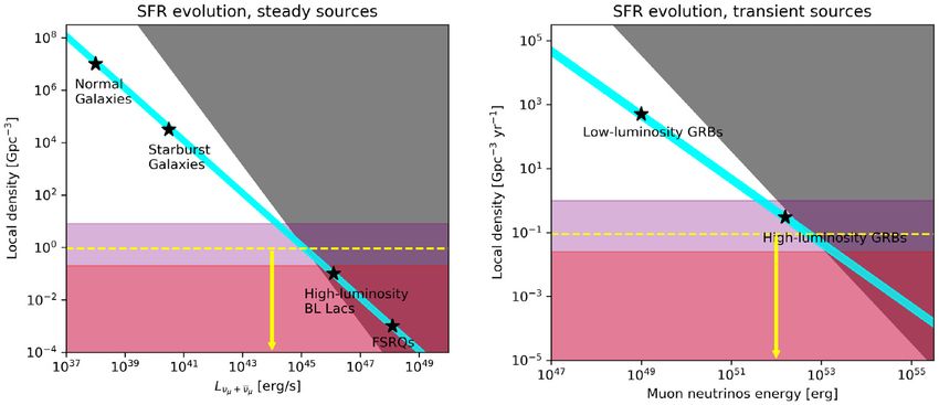
4260           A. Palladino et al.

                                                                                                                                                                Downloaded from https://academic.oup.com/mnras/article/494/3/4255/5820235 by DESY-Zentralbibliothek user on 10 September 2020
Figure 4. Neutrino multiplet constraints and the neutrino-UHECR constraints represented in the same figure. The cyan regions represent the local luminosity
density required to power the through-going muon flux measured by IceCube after 8 yr of data taking (Haack et al. 2017). The grey regions represent the
parameter space excluded by the non-observation of neutrino multiplets for the same exposure. Consequently, local densities below the yellow lines, where
these two regions intersect, are excluded. On the other hand, discovering the neutrino-UHECR correlation requires low source densities below the purple (red)
shaded regions excluding (including) the GMF in addition to the EGMF; the median 5σ discovery potential is shown. Some typical sources, according to their
evolution, are shown using stars. The different panels refer to different source evolutions and steady or transient sources, as indicated.

3 R E S U LT S                                                                       In the same figure, the grey regions denote the regions excluded
                                                                                  by the absence of neutrino multiplets in 8 yr of collected through-
We show our main result in Fig. 4 in the form in which typically the
                                                                                  going muon data by IceCube. Particularly, in this region the
neutrino multiplet limits are shown, for different source evolutions
                                                                                  probability to observe neutrino multiplets is larger than 90 per cent.
and steady or transient sources in different panels. The difference
                                                                                     Finally, the regions above the purple areas have source densities
between steady and transient sources is represented by an extra
                                                                                  that are too large for the detection of neutrino-UHECR correlations
factor, for transient sources, of (1 + z)−1 in equation (1) and the same
                                                                                  with the current sensitivities of IceCube and Auger. Concerning the
extra factor in the conversion between local density and number of
                                                                                  purple and red regions, we always assume that there are 36 neutrinos
contributing sources (see Appendix B).
                                                                                  (i.e. that the luminosity is the one required to power the through-
   In the cyan region, the product between the average source
                                                                                  going muon flux). Consequently, the allowed parameter space in
luminosity Lν (computed between 104 and 107 GeV) and the local
                                                                                  which a neutrino-UHECR correlation can be detected is marked
density ρ 0 matches the through-going muon flux detected by
                                                                                  as purple and red regions. The purple region is the one obtained
IceCube; this can be interpreted as an effective local luminosity
                                                                                  considering only the presence of the EGMF, while the red region is
density. This is obtained using a power-law flux of Eν−2.2 for each
                                                                                  the one obtained considering also the presence of the GMF, which
source (as suggested by through-going muons; Haack et al. 2017),
                                                                                  increases the average deflection.
assuming that all the sources are standard candles with the same
                                                                                     From Fig. 4, it can be read off that the possibility to observe
luminosity. The diffuse neutrino flux is then given by the following
                                                                                  correlations between neutrinos and UHECRs is restricted to a small
expression:
                                                                                  region of the parameter space of Lν and ρ 0 , when only the EGMF
dφν           zmax
                       DH L(Eν (1 + z))                                           is accounted for. In fact, if such a correlation were found, the
    =                                     ρ(z)dz,
dEν       0          4π h(z) Eν2 (1 + z)2                                         combination with the neutrino multiplet constraint would give a
                                                                                  precise measurement of the local source density and the source
where L(Eν ) is a power-law function reproducing the source
                                                                                  luminosity. The largest parameter space remains for a negative
luminosity when integrated between 104 and 107 GeV, while DH
                                                                                  source evolution (middle panels), since in that case both observed
and h(z) are defined in Appendix B. The function ρ(z) denotes the
                                                                                  particle species are produced in the nearby Universe; compare
source evolution, as represented in Fig. 1 upper left-hand panel. We
                                                                                  right-hand panels in Fig. 1. A detection of the neutrino-UHECR
then require that the diffuse flux is equal to the measured through-
                                                                                  connection would mean that the source density (for steady sources,
going muon flux, resulting in a fixed value for the product between
                                                                                  negative evolution) has to be around 10–1000 Gpc−3 , and the
the luminosity of the standard-candle sources and the local density
                                                                                  luminosity around 1044 to 1045 erg s−1 . Using the total number of
of the sources (depending on their evolution).

MNRAS 494, 4255–4265 (2020)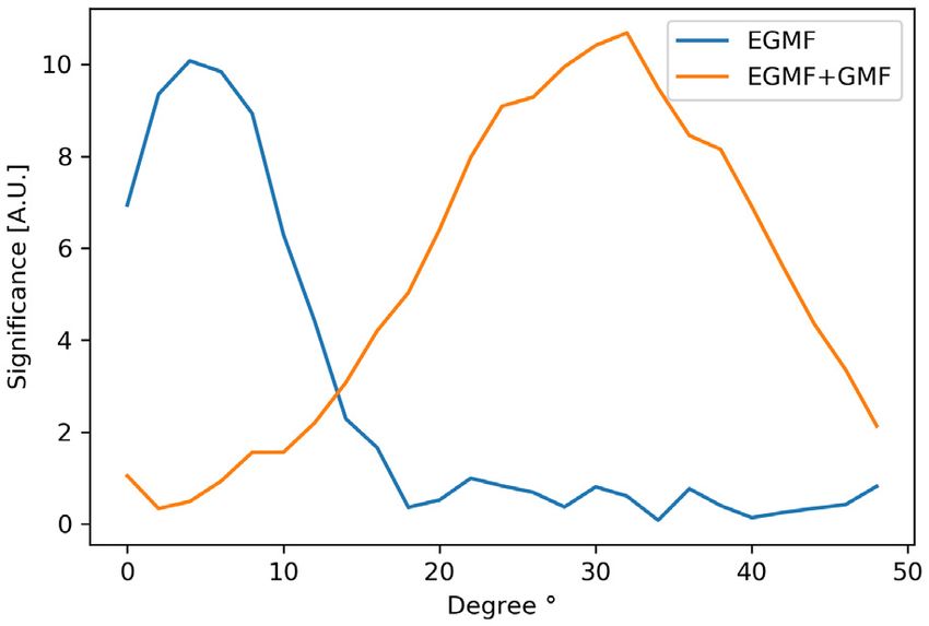
ultra-high energy cosmic rayswith UHECRs                         4261
sources as a free parameter (instead of the local density) we find            that paper have tried to span the full range of allowed EGMF models,
that the number of sources required to observe correlations Ns               from very weak to very strong EGMFs. The weakest model they
104 −105 . This number depends weakly on the source evolution,                found is, therefore, a suitable choice for the most optimistic scenario
while the local density is strongly affected by the source evolution.         for finding UHECR and neutrino correlations. The uncertainties
Indeed, fixing the total number of sources, the local density is              on the EGMF are even larger than on the GMF and a different
roughly 200 times smaller for SFR-like evolution compared to the              choice of EGMF model could give significantly larger deflections
negative evolution (see Appendix B).                                          and, therefore, less expected neutrino-UHECR correlations. The
   However, when also the GMF is considered (choosing the most                expected deflections in the case of strong EGMFs are discussed in
optimistic case, i.e. the left-hand panel of Fig. 2 that produces on          Alves Batista et al. (2017), where they show that average deflections

                                                                                                                                                        Downloaded from https://academic.oup.com/mnras/article/494/3/4255/5820235 by DESY-Zentralbibliothek user on 10 September 2020
average a smaller deflection), the possibility to observe correlations        of up to 90◦ can be reached even for protons with energies close to
becomes weak, since the required densities are already in tension             1020 eV. Such strong fields would significantly reduce the expected
with the absence of multiplets in neutrino data. Let us remark that           neutrino-UHECR correlations.
we have also optimized the analysis, changing the angular window                 Fourth, equation (1) is valid if the neutrino flux is power-
for this case, namely going from 5◦ (EGMF only) to 30◦ . Indeed,              law distributed. However, a power-law flux it is not an universal
in order to observe correlations the total number of sources must             spectrum expected in all situations. In case neutrinos are produced
not be too high, while at the same time the absence of multiplets in          by the interactions between accelerated protons and background
neutrino data suggests the opposite.                                          photons, the resulting neutrino energy spectrum has a typical bump
                                                                              shape, that differs significantly from the power-law behaviour. In
                                                                              this case it is important to verify that the peak of the energy
4 DISCUSSION
                                                                              spectrum is inside the region in which the detector is efficient.
The results presented in the previous section are obtained under              If this condition did not apply, sources that produce cosmic rays
certain assumptions, that are in most of the cases optimistic for             might produce neutrinos that are not detectable by the present
finding correlations between UHECRs and neutrinos. Even under                 experiment, which would reduce the number of effective common
these assumptions the results, considering deflections in both the            sources in our analysis. This is equivalent to the assumption that
EGMF and the GMF, are already quite pessimistic. In addition, there           only a fraction of neutrinos and cosmic rays come from the same
are some elements that we are neglecting and that can diminish the            source class; in both cases the expected number of neutrino-UHECR
expected number of neutrino-UHECR correlations even further.                  correlations goes down. This is natural to understand, since the result
    First of all, we assume that the detection probability of both            would correspond to the one presented in this work with a reduced
cosmic rays and neutrinos is equal across the entire sky. This is an          exposure, depending on the fraction of common sources.
ideal assumption, since the sky coverage of realistic experiments is             Heinze et al. (2019) shows that the UHECR fit to the spectrum and
not taken into account. Concerning the IceCube neutrino telescope,            mass composition can change significantly when choosing different
for example, track-like events (the ones with a good angular resolu-          models for hadronic interactions (EPOS LHC Pierog et al. 2015,
tion) come mostly from the Northern hemisphere, while Auger has               Sibyll 2.3 Riehn et al. 2018 or QGSJet II-04 Ostapchenko 2011)
the highest sensitivity in the Southern hemisphere. However, the              in UHECR air showers. While a different choice of one of these
inclusion of the sky coverages and detector sensitivities is beyond           models results in changes in the expected source evolution and
the purpose of this work, which aims to illustrate the possibility            spectral indices, the maximum rigidity and the composition at the
to observe correlations between neutrinos and cosmic rays under               sources are better constrained. We treat the uncertainty in the source
optimistic assumptions.                                                       evolution here by showing the results for three different scenarios,
    Secondly, we have included the GMF deflections from Farrar &              with corresponding best-fitting parameters for the spectral index,
Sutherland (2019) using the most optimistic assumption (the small-            maximum rigidity, and composition. The expected deflections in
est average deflection), represented in the left-hand panel of Fig. 2.        the EGMF mainly depend on the UHECR composition at the
The uncertainties on the GMF are still very large and if the true             sources, which is predicted rather robustly according to Heinze
GMF is close to the one represented in the right-hand panel the               et al. (2019). The deflections in the GMF model depend on the
situation will get worse. Another point to note concerning the GMF            UHECR composition at our Galaxy, which differs depending on
is that the deflections shown in Fig. 2 represent the best-fitting values     the choice of hadronic-interaction models. The best-fitting results
averaged over the full sky. In Farrar & Sutherland (2019) is shown            we used all assumed EPOS LHC as interaction model. On average,
that, in general, different deflections are expected when looking             EPOS LHC predicts a lighter composition (and therefore less
at different directions through the Galaxy. For example, according            deflections in the GMF) than Sibyll 2.3, but a heavier composition
to the parametrizations given in Farrar & Sutherland (2019), the              than QGSJet II-04. However, QGSJet II-04 does not produce a
mean separation from the source direction for R = 1018.5 V for                consistent relation between cosmic ray mass and Xmax variables
the Lcoh = 100 pc case is 45.7◦ in the Northern hemisphere,                   (Aab et al. 2014; Bellido et al. 2018) and could, therefore, be
46.8◦ in the Southern hemisphere, 28.8◦ in the Galactic plane,                considered as disfavoured. We have, however, also tested an extreme
and 40.3◦ in the full sky. Additionally, there are strong variations          scenario where we consider a pure-proton composition. Even in that
in the expected deflections depending on the exact position in                case no correlations between UHECRs and neutrinos are expected
the sky, making the separation in Northern hemisphere, Southern               when deflections in the GMF are included (see Appendix D for
hemisphere, and Galactic plane rather arbitrary. As our analysis              these results).
evaluates the discovery potential for neutrino-UHECR correlations                Besides cosmic ray–neutrino correlations and neutrino–neutrino
for all events in the full sky combined, we chose to rather use the           correlations, limits on the local source density can also be obtained
deflection distribution for the entire sky instead of separating in           from cosmic ray–cosmic ray correlations. This is what the Pierre
different sky regions.                                                        Auger Collaboration has done in Abreu et al. (2013). The limits
    Thirdly, for the EGMF the weakest model of the six models                 obtained there show that ρ 0  (0.06 − 7) × 105 Gpc−3 , even
described in Hackstein et al. (2018) has been chosen. The authors of          stronger than the limits from the neutrino multiplet constraints,

                                                                                                                 MNRAS 494, 4255–4265 (2020)
4262 A. Palladino et al.
making it even less likely that neutrino-UHECR correlations will be if the source evolution follows a similar trend. Consequently, a
found. However, the analysis presented there assumes a maximum negative source evolution, such as it may be expected for (jetted
deflection of 30◦ , while in our case often larger deflections than that or non-jetted) TDEs or low-luminosity BL Lacs, offers the best
are obtained (see Fig. 1 bottom left-hand panel and Fig. 2 left-hand perspective. Even in that case, the allowed window on the source
panel). In addition, a different minimal energy threshold for cosmic density (10–1000 Gpc−3 ) is relatively small if IceCube does not
rays is considered in Abreu et al. (2013) compared with our results find neutrino multiplets, when only the extragalactic magnetic field
(ECR ≥ 60 EeV versus ECR ≥ 1018.5 eV, respectively). It should also is considered. Adding the contribution of the Galactic magnetic
be noted that the bounds in Abreu et al. (2013) were derived from field, the required density to observe correlation has to be smaller
the lack of significant clustering in arrival directions of the highest than 10 Gpc−3 (negative evolution) – in contradiction with the non-
Downloaded from https://academic.oup.com/mnras/article/494/3/4255/5820235 by DESY-Zentralbibliothek user on 10 September 2020
energy events detected at the Pierre Auger Observatory between observation of neutrino multiplets.
2004 January 1 and 2011 December 31. By now, the number of If, on the other hand, a significant neutrino-UHECR correlation is
detected events at these energies has increased significantly and discovered, it will be an indirect precise measurement of the source
hints of anisotropies have been found (Aab et al. 2018; Caccianiga density and a strong indication for a negative source evolution,
et al. 2019), which could affect the bounds on the density of UHECR and could thus lead to the identification of the source class – and
sources. consequently to the discovery of the origin of cosmic rays. If, on
Throughout this work we have used a minimal cosmic ray energy the other hand, not even the proposed upgrade IceCube-Gen2 finds
threshold of ECR ≥ 1018.5 eV, which is roughly the energy of the neutrino multiplets within a few years of operation, the neutrino-
‘ankle’. This choice of minimal energy maximizes the number of UHECR connection will not be detected in the near future.
detected UHECRs while still making sure that most UHECRs can We conclude that the perspectives for detecting the common ori-
be expected to have an extragalactic origin and that the best-fitting gin of neutrinos and UHECRs are challenging. For example, for SFR
UHECR spectrum and composition results (Table 1) are valid. In evolution, the parameter space is already strongly constrained by the
Aartsen et al. (2016), Schumacher et al. (2019), however, 52 EeV non-observation of neutrino multiplets. Even in the best scenario,
and 57 EeV are used as minimal UHECR energy thresholds for i.e. negative source evolution, the potential to observe correlations
events detected by Auger and TA, respectively. Such a higher is limited to the possibility to observe the first neutrino multiplet
energy threshold will reduce the expected deflections of UHECRs in the very near future. If IceCube does not observe any multiplet
in magnetic fields. However, the maximum source distance from in the neutrino data in the next few years, searching for connection
which UHECRs can arrive at Earth is also reduced significantly between neutrinos and UHECRs will become meaningless.
(limiting the neutrino-UHECR even further), and the number of
detected UHECRs becomes much less. To investigate the effect of a
AC K N OW L E D G E M E N T S
higher minimal UHECR energy threshold we have redone the entire
analysis described in this paper for ECR ≥ 50 EeV, in which case the We would like to thank Andrew Taylor and Foteini Oikonomou
chance of detecting neutrino-UHECR correlations only becomes for useful discussions and Julia Tjus and Xavier Rodrigues for
smaller, see Appendix E for these results. commenting on the draft. This project has received funding from
the European Research Council (ERC) under the European Union’s
Horizon 2020 research and innovation programme (Grant No.
5 S U M M A RY A N D C O N C L U S I O N S
646623) and the Initiative and Networking Fund of the Helmholtz
We have scrutinized the question if the neutrino-UHECR connection Association.
is, in principle, detectable based on correlations of arrival directions.
To investigate the most favourable scenario, we have assumed that
all of the neutrinos in the through-going muon sample, which have REFERENCES
excellent directional resolution, and all cosmic rays above 1018.5 eV Aab A. et al., 2014, Phys. Rev. D, 90, 122005
originate from the same source class. We have taken into account Aab A. et al., 2017, J. Cosmol. Astropart. Phys., 04, 038
the different horizons of neutrinos and cosmic rays, the impact of Aab A. et al., 2018, ApJ, 853, L29
the cosmological evolution of the sources, and deflections of cosmic Aartsen M. G. et al., 2013, Science, 342, 1242856
rays in Galactic and extragalactic magnetic fields. Aartsen M. G. et al., 2016, J. Cosmol. Astropart. Phys., 01, 037
We have demonstrated that the problem of observing the Aartsen M. G. et al., 2018, Science, 361, 147
Aartsen M. G. et al., 2019a, Eur. Phys. J. C, 79, 234
neutrino-UHECR connection is intimately connected with the non-
Aartsen M. G. et al., 2019b, Phys. Rev. Lett., 122, 051102
observation of neutrino multiplets. While the non-observation of Abreu P. et al., 2013, J. Cosmol. Astropart. Phys., 05, 009
neutrino multiplets implies that the number of contributing sources Ackermann M. et al., 2019, Bull. Am. Astron. Soc., 51, 185
has to be high enough (and the corresponding luminosity low Aghanim N. et al., 2018, preprint (arXiv:1807.06209)
enough) not to detect several neutrinos from the same source, the Ahlers M., Halzen F., 2014, Phys. Rev. D, 90, 043005
neutrino-UHECR connection requires a relatively small number Ajello M. et al., 2014, ApJ, 780, 73
of sources to produce the anisotropy related to the neutrino arrival Alves Batista R. et al., 2016, J. Cosmol. Astropart. Phys., 05, 038
directions. Consequently, the non-observation of neutrino multiplets Alves Batista R., Shin M.-S., Devriendt J., Semikoz D., Sigl G., 2017, Phys.
limits the possibility to observe the neutrino-UHECR connection – Rev. D, 96, 023010
Alves Batista R., de Almeida R. M., Lago B., Kotera K., 2019, J. Cosmol.
if it exists.
Astropart. Phys., 01, 002
We have found that the best scenario for finding the neutrino-
Baerwald P., Bustamante M., Winter W., 2015, Astropart. Phys., 62, 66
UHECR connection are sources with a negative source evolution. Bellido J.Pierre Auger Collaboration, et al., Pierre Auger Collaboration,
That is easy to understand: Since the UHECR horizon is limited 2018, Proc. Sci., ICRC2017, 506
by photo-hadronic interactions (such as photo-disintegration) with Berezinsky V. S., Zatsepin G. T., 1969, Phys. Lett., 28B, 423
the cosmic background light, there is the most statistical overlap Caccianiga L.Pierre Auger Collaboration, et al., Pierre Auger Collaboration,
with the neutrinos (which can travel through the whole Universe) 2019, Proc. Sci., ICRC2019, 206
MNRAS 494, 4255–4265 (2020)ultra-high energy cosmic rayswith UHECRs 4263
Farrar G. R., Sutherland M. S., 2019, J. Cosmol. Astropart. Phys., 05, with
004
Fenu F.Pierre Auger Collaboration, et al., Pierre Auger Collaboration, 2018, h(z) = λ + m (1 + z)3
Proc. Sci., ICRC2017, 486
and λ = 0.685, m = 0.315, following Aghanim et al. (2018).
Haack C.IceCube Collaboration, et al., IceCube Collaboration, 2017, Proc.
Therefore, the comoving volume is given by:
Sci., ICRC2017, 1005
Hackstein S., Vazza F., Brüggen M., Sorce J. G., Gottlöber S., 2018, 4
MNRAS, 475, 2519 Vc = π Dc3
3
Heinze J., Boncioli D., Bustamante M., Winter W., 2016, ApJ, 825,
122
and the derivative in z is equal to:
Downloaded from https://academic.oup.com/mnras/article/494/3/4255/5820235 by DESY-Zentralbibliothek user on 10 September 2020
Heinze J., Fedynitch A., Boncioli D., Winter W., 2019, ApJ, 873, 88 dVc d 2 (z)
Jansson R., Farrar G. R., 2012a, ApJ, 757, 14 = 4π DH3 .
dz h(z)
Jansson R., Farrar G. R., 2012b, ApJ, 761, L11
Kistler M. D., Yuksel H., Beacom J. F., Hopkins A. M., Wyithe J. S. B., In addition, we define the luminosity distance, that takes into
2009, ApJ, 705, L104 account the redshift energy loss, as D (z) = Dc (z)(1 + z).
Kowalski M., 2015, J. Phys. Conf. Ser., 632, 012039 Given the source density per comoving volume ρ(z), the contri-
Murase K., Waxman E., 2016, Phys. Rev. D, 94, 103006 bution to the neutrino luminosity is given by:
Ostapchenko S., 2011, Phys. Rev. D, 83, 014018
Pierog T., Karpenko I., Katzy J. M., Yatsenko E., Werner K., 2015, Phys. −1 dVc 1
fν (z) = f˜ν ρ(z) ,
Rev. C, 92, 034906 dz D2 (z)
Riehn F., Dembinski H. P., Engel R., Fedynitch A., Gaisser T. K., Stanev T., z
2018, Proc. Sci., ICRC2017, 301 with f˜ν = 0 max dz ρ(z) dV c 1
dz D2 (z)
, where we choose zmax = 5 (the
Schumacher L.or the ANTARES, IceCube, Pierre Auger, Telescope Array exact value chosen for zmax is irrelevant for the final results as long
Collaborations, et al., or the ANTARES, IceCube, Pierre Auger, Tele- as zmax 3). For transient sources the previous equations have an
scope Array Collaborations, 2019, EPJ Web Conf., 207, 02010 extra factor (1 + z)−1 , as discussed in Kistler et al. (2009). The
Sun H., Zhang B., Li Z., 2015, ApJ, 812, 33
functions fν (z), for the three different cases, are shown in the upper
Yuksel H., Kistler M. D., Beacom J. F., Hopkins A. M., 2008, ApJ, 683, L5
right-hand panel of Fig. 1.
A P P E N D I X A : S O U R C E E VO L U T I O N
APPENDIX B: NUMBER OF SOURCES VERSUS
In this section we analyse the contribution to the flux of neutrinos LOCAL DENSITY
and cosmic rays as a function of redshift, assuming different
The local density ρ 0 and the total number of sources Ns are
cosmological evolutions of the sources, namely a negative, a flat, and
connected to each other and the constant of proportionality depends
an SFR evolution. We define these three different source evolutions
on the source evolution. The relation between these two quantities
per comoving volume ρ(z), as follows:
can be expressed as follows (see e. g. Baerwald, Bustamante &
(i) sources are characterized by having a negative source evolu- Winter 2015 for an extended discussion):
tion, i.e. the amount of nearby sources is larger than the amount of Ns
distant sources. For this case we assume ρ(z) ∝ (1 + z)−3 , based ρ0 = ,
4π DH3 hz
on Sun et al. (2015);
(ii) A flat evolution. The sources are uniformly distributed with where
redshift. zmax
1 ρ(z) dVc
(iii) The source distribution follows the SFR. In this case the hz = τ (z)dz,
4π DH3 0 ρ(z = 0) dz
evolution is characterized by
⎧ here we assume zmax = 5, DH is the Hubble distance and ρ(z)
⎪
⎪ (1 + z)3.4 for z < 1 the source evolution as defined in Section A. For steady sources
⎨
ρ(z) ∝ (1 + z) −0.3
for 1 ≤ z ≤ 4 , τ (z) = 1 while τ (z) = 1/(1 + z) for transient sources. The value
⎪
⎪ of hz changes according to the source evolution and the topology
⎩ −3.5
(1 + z) for z > 4 of the source. In the case of steady sources, we obtain hz = 0.1 for
according to Yuksel et al. (2008). negative evolution, hz = 2.2 for flat evolution, and hz = 18.0 for
SFR evolution.
The three source distributions ρ(z) are represented in the upper
left-hand panel of Fig. 1 as a function of redshift.
In order to compute the contribution to the neutrino flux, given a APPENDIX C: SCAN ON THE ANGULAR
certain source distribution, we need to introduce some elements of W I N D OW
cosmology. First of all we define the comoving distance as: To determine what the optimal angular window is to search for
Dc (z) = DH × d(z), correlations between UHECRs and high energy neutrinos, we
perform a scan using different values for the angular window. We
where DH = c/H0 , with H0 = 67.3 km/s Mpc
and DH = 4.46 Gpc repeat the scan for two scenarios, i.e. extragalactic magnetic field
(Aghanim et al. 2018). The function d(z) is defined as: only and extragalactic+Galactic magnetic fields. For this purpose
z we simulate 103 sky maps, using SFR and a local density of 1 Gpc−3 ,
dz
d(z) = , because in this scenario correlations are guaranteed (see upper right-
0 h(z ) hand panel of Fig. 4). See Fig. C1 for the results of this scan.
MNRAS 494, 4255–4265 (2020)4264 A. Palladino et al.
A P P E N D I X D : P U R E - P ROT O N C O M P O S I T I O N
In this section we evaluate the effect of a different cosmic ray
composition, using purely protons and the same energy threshold
used in the main text, i.e. protons above 1018.5 eV. Although this
scenario has already been excluded by the Auger measurements, it
is instructive as it is the most optimistic case in terms of UHECR-
neutrino connections, since protons are deflected less than heavier
nuclei. We did this for sources following the SFR with best-fitting
Downloaded from https://academic.oup.com/mnras/article/494/3/4255/5820235 by DESY-Zentralbibliothek user on 10 September 2020
values for γ = 2.42 and Rmax = 1021.9 V obtained from Heinze et al.
(2016). The angular window for finding correlations between high
energy neutrinos and UHECRs has been optimized for this specific
scenario. For the EGMF only, the optimal angular window is 3◦ ,
Figure C1. Search for the optimal angular window to observe connections while for EGMF+GMF the optimal angular window is 15◦ . The
between UHECRs and high energy neutrinos, assuming deflections in results are represented in Fig. D1. However, even in this extreme
the extragalactic magnetic field only (blue line) and adding the Galactic case, once the Galactic magnetic field is taken into account, the
magnetic field (orange line).
possibility to find correlations between UHECRs and high energy
neutrinos in disfavoured.
Figure D1. As in Fig. 4, for a scenario with protons only and a minimal cosmic ray energy threshold of 1018.5 eV. An SFR source evolution is implemented.
MNRAS 494, 4255–4265 (2020)ultra-high energy cosmic rayswith UHECRs 4265
UHECRs come only from the very local Universe, while neutrinos
A P P E N D I X E : C O S M I C R AY S A B OV E 5 0 E E V
can come also from distant sources (see upper panels of Fig. 1).
The entire analysis proposed in this paper, using cosmic rays above As a consequence, although at higher energies cosmic rays are
1018.5 eV, has been repeated using a subset of cosmic rays with less deflected, the cosmological connection with neutrinos is lost.
energies above 50 EeV. In this energy range ∼300 cosmic rays have Repeating the analysis with cosmic rays above 50 EeV, we obtain
been detected by Auger. Roughly this energy threshold is often the results reported in Fig. E1. In order to observe correlations the
used to search for correlations between cosmic rays and neutrinos, local density should be much smaller than in the scenario with
since it is commonly believed that at this energy the deflection ECR > 1018.5 eV (Fig. 4); this suggests that 1018.5 eV would be a
for cosmic rays is small and correlations with neutrinos are more more appropriate cosmic ray energy threshold for neutrino-UHECR
Downloaded from https://academic.oup.com/mnras/article/494/3/4255/5820235 by DESY-Zentralbibliothek user on 10 September 2020
likely observed. However, at these very high energies the observed correlation searches.
Figure E1. As in Fig. 4 using an energy threshold of 50 EeV.
This paper has been typeset from a TEX/LATEX file prepared by the author.
MNRAS 494, 4255–4265 (2020)You can also read