High resolution tsunami inversion for 2010 Chile earthquake
←
→
Page content transcription
If your browser does not render page correctly, please read the page content below
Nat. Hazards Earth Syst. Sci., 11, 3251–3261, 2011
www.nat-hazards-earth-syst-sci.net/11/3251/2011/                                                  Natural Hazards
doi:10.5194/nhess-11-3251-2011                                                                          and Earth
© Author(s) 2011. CC Attribution 3.0 License.                                                    System Sciences

High resolution tsunami inversion for 2010 Chile earthquake
T.-R. Wu and T.-C. Ho
Graduate Institute of Hydrological and Oceanic Sciences, National Central University, Jhongli, Taiwan
Received: 2 March 2011 – Revised: 14 August 2011 – Accepted: 4 October 2011 – Published: 12 December 2011

Abstract. We investigate the feasibility of inverting high-        deformation was about 4 to 5 m. On the other hand, the
resolution vertical seafloor displacement from tsunami wave-       tsunami signal recorded by the buoys and tidal gauges around
forms. An inversion method named “SUTIM” (small unit               the epicenter might open us a window to understand the
tsunami inversion method) is developed to meet this goal.          seafloor displacement and earthquake characteristics.
In addition to utilizing the conventional least-square inver-         Tsunami is a gravity wave generated mainly by earth-
sion, this paper also enhances the inversion resolution by         quakes and landslides. A strong earthquake occurring in the
Grid-Shifting method. A smooth constraint is adopted to            ocean is often accompanied by tsunamis. Because the wave-
gain stability. After a series of validation and performance       length is much longer than the water depth, tsunami is cate-
tests, SUTIM is used to study the 2010 Chile earthquake.           gorized as a pure linear wave which obeys the shallow water
Based upon data quality and azimuthal distribution, we se-         equation (SWE) in wave propagation. In addition, the wave
lect tsunami waveforms from 6 GLOSS stations and 1 DART            propagation speed is much slower than the seafloor move-
buoy record. In total, 157 sub-faults are utilized for the high-   ment, therefore the initial tsunami profile, or the tsunami
resolution inversion. The resolution reaches 10 sub-faults         source, can be treated as the seafloor vertical displacement
per wavelength. The result is compared with the distribu-          (Wu et al., 2009; Megawati et al., 2009; Huang et al., 2009;
tion of the aftershocks and waveforms at each gauge location       Saito and Furumura 2009). Once the tsunami initial free-
with very good agreement. The inversion result shows that          surface profile is inverted from the wave gauges, some fault
the source profile features a non-uniform distribution of the      parameters can be determined. Compared to the conven-
seafloor displacement. The highly elevated vertical seafloor       tional seismic inversion method, the tsunami inversion re-
is mainly concentrated in two areas: one is located in the         quires only wave signals and bathymetry data, which can be
northern part of the epicentre, between 34◦ S and 36◦ S; the       accessed relatively easily.
other is in the southern part, between 37◦ S and 38◦ S.
                                                                      This idea is not new; Satake (1987) proposed a tsunami in-
                                                                   version method to infer the seismic parameters from the tidal
                                                                   gauge data. His method was further used on the tsunami fore-
1   Introduction                                                   cast (Wei et al., 2003; Yamazaki et al., 2005) and exploration
                                                                   of earthquake events with sea surface deformation (Pires and
The 2010 Chile earthquake occurred off the coast of the            Miranda 2001; Baba et al., 2002, 2005; Satake et al., 2005;
Maule Region on 27 February 2010, registering a magni-             Piatanesi and Lorito 2007). However, those implementa-
tude of 8.8 on the moment magnitude scale (USGS). In               tions used very large unit sources such that the details of the
this event, the segment of the fault zone was estimated            tsunami profiles could not be described. With the advance of
to be between 500 km to 700 km long with an average                fast computation and modern tidal gauge facilities, the small
slip about 10 m (USGS, BGS). A precise GPS measure-                unit inversion method becomes feasible. Saito et al. (2010)
ment (http://researchnews.osu.edu/archive/chilemoves.htm)          used small unit sources to study the 2004 earthquake off Kii
showed that several cities south of Cobquecura were raised         Peninsula with a reasonably good result. In their paper, they
by up to 3 m at least. Lorito et al. (2011) and Fritz              emphasized the importance of dispersion effect to the small-
et al. (2011) further estimated that the maximum surface           scale tsunamis. However, no performance tests and model
                                                                   validations were presented in their studies. In this paper,
                                                                   we introduce the small unit source tsunami inversion method
                     Correspondence to: T.-R. Wu                   (SUTIM) to rebuild the fine structure of tsunami source. In-
                     (tsoren@ncu.edu.tw)                           stead of using the Gaussian distribution (Saito et al., 2010),

Published by Copernicus Publications on behalf of the European Geosciences Union.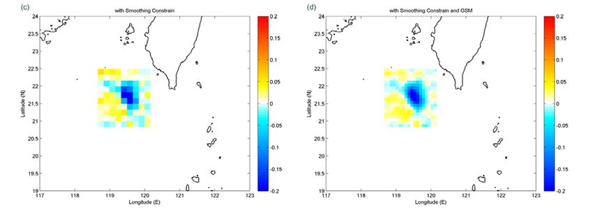
3252                                     T.-R. Wu and T.-C. Ho: High resolution tsunami inversion for 2010 Chile earthquake

1
2 Fig. 1.   The procedure of SUTIM.

3 the Figure   1. The
      top-hat small unit procedure    of SUTIM.
                         sources are adopted to maintain the
                                                                    ∂η
                                                                       + ∇ × [(h + εη)u] = 0,                                   (1)
    mass conservation. To save computational costs, moreover,       ∂t
4   a grid shifting method is proposed. To ensure the stability     ∂u
    of the inversion result, the smoothing constraint is applied.      + εu × ∇u + ∇η = 0.                                      (2)
                                                                    ∂t
    In the present model, the wave dispersion effect is assumed
    to be small and negligible. To evaluate the performance of      Equation (1) is the continuity equation and Eq. (2) is the
    SUTIM, a fictitious earthquake event is created as the bench-   momentum equation, in which h represents the local water
    mark problem. Last, the SUTIM is utilized to study a real       depth, η is wave height, t is time, u is the horizontal velocity
    event: the 2010 Chile Earthquake. The result is presented       vector, and ε is the nonlinearity defined as ε = a/ h, a is the
    and discussed in this paper.                                    wave height. If ε < 1/20, the wave is categorized as a linear
                                                                    shallow water wave and the terms with ε can be omitted.
                                                                       Another important parameter used to define the dispersion
    2     Algorithm
                                                                    effect is dispersion coefficient, µ, defined as µ = h/λ, in
    2.1    Shallow water equation and COMCOT Numerical              which λ is wavelength. If µ < 0.05, the wave is a nondisper-
           model                                                    sive shallow water wave and can be described by SWE (Dean
                                                                    and Dalrymple, 1991). In general, an earthquake tsunami
    The wave motion can be described by the potential flow the-     propagating in the deep ocean is a typical linear and non-
    ory. By integrating the equations along the water depth, the    dispersive wave. Both nonlinear and dispersion effects can
    shallow water equation can be derived (Dean and Dalrym-         be ignored.
    ple, 1991). Equations (1) and (2) are the nonlinear SWE in a       To calculate the tsunami propagation, a SWE code named
    non-dimensional form.                                           COMCOT is utilized to perform the calculation. COMCOT
                                                                    is able to solve both linear and nonlinear shallow water equa-
                                                                    tions in Cartesian or Spherical coordinate systems. It has
                                                                    been widely used to study many historical tsunami events,

    Nat. Hazards Earth Syst. Sci., 11, 3251–3261, 2011                        www.nat-hazards-earth-syst-sci.net/11/3251/2011/
T.-R. Wu and T.-C. Ho: High resolution tsunami inversion for 2010 Chile earthquake 3253
1
2 Fig.
Figure 3. Gauge
3. Gauge locationlocation and bathymetry
and bathymetry profile used in profile used intestthe
the performance of perfor-
SUTIM.
3 mance test of SUTIM.
2. Decide the inverse region. Although this region has
to cover the entire possible tsunami source area, using
smaller coverage can save computational time and con-
strain the uncertainty of inversion.
3. Place a series of unit sources over the inverse region.
1 Fig. 2. The sketch of grid shifting. The 1st layer of unit source array Each unit source shares the same wave height, which is
is presented in solid lines. The 2nd layer is presented in dashed a unit.
2 lines. The shaded area is the final resolution by applying the grid
shifting method. st 4. Calculate the wave propagation of each unit source, and
3 Figure 2. The sketch of grid shifting. The 1 layer of unit source array is presented in solid
record the computed waveforms at each gauge.
4 lines. The 2nd layer is presented in dashed lines. The shaded area is the final resolution by
such as the 1992 Flores Islands tsunami (Liu et al., 1994, 5. Adjust the initial wave height by multiplying the
5 applying the grid
1995), 2004shifting
Indian method.
Ocean tsunami (Wang and Liu, 2006, weighting factor, and sum the adjusted gauge results to-
6 2007), and 2006 Pingtung tsunami (Wu et al., 2008; Chen et gether to have the best fit to the real gauge record. We 19
al., 2008). The accuracy reaches the 2nd order in both spatial adopt the least square method to obtain the best-fit re-
and time domains. COMCOT also supports the nested grid sult.
system that allows the finer grid to be placed on a coarser
grid to increase local resolution. 6. Apply the grid shifting method to increase the resolution
of the tsunami source.
2.2 Tsunami inversion method
In the following sections, the detailed algorithm of SUTIM
will be described.
The energy of a tsunami wave can be accumulated linearly
because of its linear characteristic. In other words, the wave
2.3 Least square method
energy can be divided into many small units and superposed
back on the original one, i.e. each element of vertical dis- In SUTIM, the numerical gauges record the computed wave-
placement is deduced numerically without referring to any forms from each unit source. By comparing the results with
dislocation formulation. Upon the linear superposition the- field data, a best-fit weighting matrix can be determined. The
ory and the least square method, SUTIM is developed. The weighting matrix is a factor matrix for the unit source array
algorithm used in SUTIM is shown in Fig. 1 and below: and the multivariable least square method is utilized. We set
matrix a as the factor matrix of the unit source array. The
1. Select waveforms from buoys or tidal gauges. Judg- linear matrix-vector equation is shown in Eq. (3). The first
ing by the data quality and azimuthal distribution, we lower-index indicates the data
18 number. The second index in-
choose the proper wave gauges to perform the inversion. dicates the number of the unit source. Vector b is the obser-
The gauges close to the source region with deeper local vation gauge data. Vector x is the weighting factor, which
water depth and less site effects are preferred. will be solved by the least square method. Constant m is the
www.nat-hazards-earth-syst-sci.net/11/3251/2011/ Nat. Hazards Earth Syst. Sci., 11, 3251–3261, 20113254 T.-R. Wu and T.-C. Ho: High resolution tsunami inversion for 2010 Chile earthquake
Table 1. The fault parameters of fictitious earthquake and 2010 Chile earthquake.
Latitude Longitude Strike Dip Slip Depth Length (centroid) Width Dislocation
(E) (N) (deg.) (deg.) (deg.) (km) (km) (km) (m)
Fictitious Earthquake 119.5 21.5 165 30 −76 19.6 35.77 17.88 2
2010 Chile Earthquake −35.98 −73.15 19 18 116 23.2 500 100 10
total number of the unit source, and n is the total number of 2.5 Multi-event inverse
the gauge data.
a11 x1 + a12 x2 + ··· + a1n xn = b1 In some earthquake events, multiple earthquakes happened in
a21 x1 + a22 x2 + ··· + a2n xn = b2 a short period. The 2006 Pingtung earthquake doublet is one
.. . (3) example. Two earthquakes with similar magnitude occurred
. within 8 min. In such case, both events shall be included in
am1 x1 + am2 x2 + ··· + amn xn = bm the tsunami inversion. In the multi-event approach, we create
unit sources with multiple events, and then calculate all the
Equation (3) can be rewritten in a matrix form:
wave propagation of each unit source.
b1 In the case of the multi-event, the observation data b has
a
a11 12 ··· a1n x1 b2 the combined influence from all events, and therefore the cal-
a21 a22 . . . a2n x2
. culated wave height shall be the summation of each multi-
. .
= .. . (4)
. .. . . .. .
unit source:
. . . .
. .
..
am1 am2 ··· amn xn After composing all the unit source results, the modified
bm linear matrix-vector equation can be derived. Equation (7)
Based on the least square method, the weighting vector x can shows the example of two events.
be acquired by solving Eq. (5):
−1 x1
x = AT A AT b. (5)
a11 ··· a1n a1n+1 ··· a1n+n
.
b1
..
.. . . .. .. .. .. ..
Equation (5) is the standard formula of the least square . . . . . . xn
.
.. . . .. .. . .. ,
= (7)
method used to invert the equation. However, this method .. xn+1
..
. . . . . .
.
has to be modified for the multi-gauge and multi-event cases. ··· aMn+n ..
aM1 ··· aMn aMn+1 bM
Because the least square method suffers from the unstable | {z }| {z } x
n+n
(Event 1) (Event 2)
and non-physical features, in which case a smoothing con-
straint is required in the following sections.
in which the elements from a11 to a1n represent the gauge
2.4 Multi-gauge inversion data of the first event, and elements from a1 n + 1 to a1n+n
represent the gauge data of the second event. x1 to xn are
In most of the real tsunami events, more than one wave gauge the weighting factors of the first event. xn+1 to xn+n are
or buoy record will be used to perform the tsunami inversion. the weighting factors of the second event. b1 to bM are the
When multiple gauges are employed in the inversion method, observed data containing signals of both two events.
Eq. (4) can be extended as follows:
a11 ··· a1n b1 2.6 Smoothing constraint
.. .. .. ..
. . . .
am1 ··· amn bm
Based on the seismic theory and field observations, the sur-
x1 face of the ground movement should be smooth (Hartzell
am+11 ··· am+1n
.. bm+1
.. . . = . , (6) and Heaton, 1983). However, the seafloor profile inverted
. .. .. .
..
xn directly from the tsunami inversion might be bumpy and
am+m1 ··· am+mn bm+m non-physical, a smoothing constraint is required. Adding a
. .. .. . smoothing constraint as a damping function has been widely
.. .
. . .
used in the seismic inversions (Yen et al., 2008; Lee et
aM1 ··· aMn bM
al., 2008) and some tsunami inversions (Baba et al., 2005;
in which m represents the total number of combined data. Saito et al., 2010). The smoothing constraint constrains each
Nat. Hazards Earth Syst. Sci., 11, 3251–3261, 2011 www.nat-hazards-earth-syst-sci.net/11/3251/2011/T.-R. Wu and T.-C. Ho: High resolution tsunami inversion for 2010 Chile earthquake 3255
1
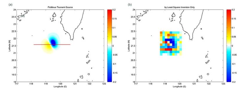
Fig. 4. The
2 tsunami source profiles. (a) Fictitious tsunami source. (b) by Least square inversion only. (c) with smoothing constraint. (d) with
smoothing constraint and GSM. The white line in (a) shows the cross-section used in Fig. 5.
3 Figure 4. The tsunami source profiles. (a) Fictitious tsunami source. (b) by Least square
tsunami4 unitinversion
source to have
only.a relationship with its neighbor-
(c) with smoothing constraint. (d) with smoothing constraint and GSM. The
ing unit source as:
5 white line in (a) shows the cross-section used in Figure
a111 ··· 5.a123 ··· a132 a133 a134 ··· a143 ··· a1ij
.. .. .. .. .. .. .. .. .. .. ..
k . . . . . . . . . . .
k × swt6× xs =
X
(swt × xi ), (8) aM11 ··· aM23 ··· aM32 aM33 aM34 ··· aM43 ··· aMij
i=1 0 ··· −1 × swt ··· −1 × swt 4 × swt −1 × swt ··· −1 × swt ··· 0
b1
in which xs is the weighting factor of one specific unit source, xi1 .
xi represents the weighting factor of neighboring units of the .. ..
. = , (10)
specific unit. k is the total number of neighboring unit source bM
xij
on xs , and swt is the smoothing weight scalar. Thus, each unit 0
has defined relationship with its neighboring units. For ex-
ample, considering one specific tsunami unit source 33 with in which i and j are the IDs of the unit source, M is the
the neighboring units 32, 34, 23, and 43, the equation of the length of data, and swt is the smoothing strength. With this
smoothing constraint can be written as: constraint, each unit source builds up the relationship with its
neighboring units, and the result will be smoothed.
4 × swt × x33 = swt × x23 + swt × x43 + swt × x32 + swt × x34 . (9)
2.7 Grid Shifting Method (GSM)
in which x33 represents the weighting factor of unit 33, and
unit 32, 34, 23, 43 are x32 , x34 ,x23 , and x43 . The swt is the In order to reproduce the detail of the source distribution, a
smoothing strength. Equation (9) can be added to the matrix large number of unit sources have to be applied to the possi-
a as shown in Eq. (10): ble tsunami source region. Each unit source requires 20 grid
points to resolve the wave propagation. Therefore, double
resolution requires quadruple unit sources, not to mention
using a finer grid size and smaller time steps. The
20 calcula-
tion is very time consuming even on modern computers. In
www.nat-hazards-earth-syst-sci.net/11/3251/2011/ Nat. Hazards Earth Syst. Sci., 11, 3251–3261, 20113256 T.-R. Wu and T.-C. Ho: High resolution tsunami inversion for 2010 Chile earthquake
1
2
Fig. 5. The cross-section profiles of the tsunami source. (a) Fic-
3 Figure 5. The cross-section profiles of the tsunami source. (a) Fictitious tsunami source. (b)
titious tsunami source. (b) by Least square inversion. (c) with
4 by Least square inversion.
smoothing (c) with
constraint. smoothing
(d) with constraint.
smoothing (d) with smoothing
constraint and constraint and
1 GSM.
5 GSM. Fig. 6. The computational domain, bathymetry, gauge location
6 2 (marked in white triangle), epicenter of the 2010 Chile earthquake
this study, we propose the grid shifting method to enhance
3 Figure 6. The(marked in red asterisk),
computational tsunami source
domain, bathymetry, from
gauge Okada (marked
location model (drawn
in white triangle),
the source resolution with limited extra CPU load. in contour lines with 1m interval), and the unit sources (drawn in
The grid shifting method is described as follows: 4 epicenter of the 2010
small redChile earthquake
squares). (marked
The color in redthe
bar shows asterisk), tsunami
bathymetry source from Okada
in meters.
5 model (drawn in contour lines with 1m interval), and the unit sources (drawn in small red
1. Create the first layer of unit source array as previously
6 squares). The color bar shows the bathymetry in meters.
described. of the computational load. We shall demonstrate the perfor-
7
2. Create the second layer of unit source array identical mance of GMS in the following sections.
to the first one. However, we slightly shift the second
unit source array with 1/2 grid spacing (Fig. 2). As the 2.8 Restriction in SUTIM
result, there is an overlapped area where the resolution
is 1/2 of the original one. Several assumptions are made for SUTIM; we shall list all
the limitations while using it.
3. Calculate the wave propagation of both unit source ar-
21
rays, and perform the least square method to find the
weighting factors on both arrays. 1. The tsunami has to be a linear water wave, which obeys
a/ h < 1/20.
4. Average both weighting factors on each overlapped unit
source.
2. The tsunami has to be a long water wave, which follows
The idea of grid shifting method is that the two-layer unit h/λ < 0.05.
sources shall be able to capture more detailed information 22
than just one-layer ones. Shifting the unit sources by half
grid spacing indicates that the sampling resolution is dou- 3. The tsunami source is large and the slip duration is
bled. Because the size of the unit source is larger than the short. One of the important assumptions used in SU-
sampling resolution, we average both layers to obtain the fi- TIM is that the vertical component of seismic motion
nal solution. This might raise an issue of over-smoothing is the same as the tsunami source. However, it is not
problem. However, the grid-shifting method indeed provides always true. Saito and Furmura (2009) proposed the
detailed information of tsunami source profile. The good per- limitation to this assumption. The criteria are λ
13h
formance of this method can be seen in the following sec- and T
λ/(8c), in which T is slip duration, and c is
tions. the phase velocity of the tsunami. In other words, the
As the length of averaged result on each unit source is 1/2 length of source has to be much longer than the water
of the original unit source, the inversed tsunami source has depth, and the duration of seismic motion has to be very
finer resolution and the calculation requires only the double short to ensure this assumption is correct.
Nat. Hazards Earth Syst. Sci., 11, 3251–3261, 2011 www.nat-hazards-earth-syst-sci.net/11/3251/2011/T.-R. Wu and T.-C. Ho: High resolution tsunami inversion for 2010 Chile earthquake 3257
Fig. 7. Waveform comparisons. Solid lines: simulated waveforms with traditional tsunami source determination method. Dotted lines: field
measurements.
3 Result and discussion Figure 4c is the result after the smoothing constraint is ap-
plied. The inversed tsunami source is smoother compared to
3.1 Performance Test of SUTIM Fig. 4b. However, the low-resolution issue still exists. Fig-
ure 4d shows the results after the adoption of both smoothing
In order to examine the performance of SUTIM, a fictitious constraint and GSM. The source profile is much cleaner than
tsunami event is created as shown in Fig. 3a. The size of the that in Fig. 4b and c. The surface is smooth and the reso-
fictitious source region is 172.7 km by 155.4 km, located at lution is high enough to easily identify the elevation and the
100 km off Taiwan. The source profile is generated by the strike angle. The inversion result is very close to the fictitious
half-space semi-elastic model (Okada, 1985) with the fault source. Figure 5 shows the comparisons on the cross-section
parameters listed on Table 1. Figure 3 shows the bathymetry in Fig. 4a. The cross-section is located at 21.5◦ N and extends
profile as well as the gauge location. The wave gauges are from 118.5◦ E to 120.4◦ E. As seen in Fig. 5b, although SU-
all placed in the southern part of Taiwan. The ill-deployed TIM fails to predict the flat surface between 118.5◦ E and
gauges and complex bathymetry raise the difficulty for the 119.0◦ E, the steep slope near 119.4◦ E can still be easily
inversion. The maximum surface elevation of the source is identified. This results from the low resolution of the unit
0.049 m and −0.243 m with local water depth about 2500 m source. Figure 5c shows the smoothed result, and Fig. 5d
(Fig. 4a). The fictitious source profile is smooth, yet the shows the final result with smoothing constraint and GSM.
result from SUTIM will be a stair-like profile, which adds The result indicates that, with the smoothing constraint and
some uncertainties to the inversion. Figure 4b is the in- GSM, SUTIM can improve the quality of the inversion re-
version result directly from the least square method. Al- sults.
though the negative and positive tsunami sources as well as
the strike angle can be roughly identified, the coarse res-
olution makes recognition difficult and the surface bumpy.
www.nat-hazards-earth-syst-sci.net/11/3251/2011/ Nat. Hazards Earth Syst. Sci., 11, 3251–3261, 20113258 T.-R. Wu and T.-C. Ho: High resolution tsunami inversion for 2010 Chile earthquake
1 1
2 Fig. 8. Inversion result by SUTIM of 2010 Chile earthquake. 2 (a) by Fig. 9. (a) The inversion result with SUTIM of vertical displace-
Least square ment and aftershocks of the 27 February 2010 event. (b) the in-
3 Figure 8. Inversion resultinversion
by SUTIMand smoothing
of 2010 constraint.(a)(b)
Chile earthquake. by with
Least GSM. inversion
3 square
Figure 9. (a) The inversion resultSUTIM
with SUTIM of vertical displacement andtsunami
aftershocks of the
Color bar indicates the vertical displacement of the seafloor in me- version results with in gray and from traditional
4 and smoothing constraint. (b) with GSM. Color bar indicates the vertical 4displacement of
February 27,the
source
2010determination method presented
event. (b) the inversion in SUTIM
results with counterinlines.
gray The blue traditional
and from
ters.
5 seafloor in meters. 5 tsunami source circle determination
is the epicenter location
method reportedinbycounter
presented Globallines.
CMT.The blue circle is the
6 6 epicenter location reported by Global CMT.
3.2 2010 Chile earthquake
7 7 We refer this method to the traditional source-determination
Before applying the SUTIM to the event of 2010 Chile earth- method. Figures 6 and 7 show the tsunami source and the
quake, we shall inspect the restrictions that require parame- gauge comparisons, respectively. We can see that the tsunami
ters, a, h, λ, and T . The possible wave height a is assumed source from the traditional source determination is smooth
to be 3 m estimated from the GPS measurement in the south and uniform spatially. However, the source profile does not
of Cobquecura. The local water depth h varies from 500 m seem natural. The calculated waveforms shown in Fig. 7 are
to 3000 m. To ensure the inversion quality, h = 500 m is simulated by COMCOT. In Fig. 7, although the arrival time
adopted. The wavelength or the length of the source λ can of the first peak is predicted correctly, the detailed waveforms
be deduced from the distribution of the aftershocks. In this deviate from the field data. This indicates that the source lo-
case, it is estimated to be 100 km. The source duration or the cation is correct, yet the source profile is not.
rise time T can be estimated from slip divided by slip veloc-
ity. The slip is about 10 m from BGS, and the slip velocity is 3.2.2 Source inversion using SUTIM
about 1 m s−1 in most of the earthquake events. The source
duration T is therefore estimated to be 10 s. We apply forty-five unit sources to the first layer and fifty-
Based on the above mentioned parameters, the character- three unit sources to the second layer for GSM. The size of
istics of the tsunami source can be determined: a/ h = 0.006, each unit is a 400 × 400 square. Six gauges are chosen from
smaller than 1/20; h/λ = 0.005, which is smaller than 0.05; GLOSS (The Global Sea Level Observing System) and one is
λ = 100 m
h = 500 m; and T = 10 s
λ/(8c) = 178 s. from NDBC DART station as shown in Fig. 6. Figure 6 also
24 25
We conclude that SUTIM is suitable for studying the 2010 shows the computation domain and unit sources. Figure 8b
Chile earthquake. shows the inversion result with GSM and smooth constraint.
In the figure we can see the seafloor displacement distributes
3.2.1 Parameter predetermination non-uniformly. Two primary clusters of positive elevation
can be observed. One cluster distributes along the coastline
To employ SUTIM, the possible source region has to be de- between 35◦ S and 36◦ S, which is the asperity of this event.
termined a priori. Based on the seismic report from USGS The maximum elevation is 3.63 m, which is very close to the
website and aftershocks reported from Global CMT, the GPS measurement. The other is weaker and distributed in
length is estimated to be 500 km. The rupture width is as- the south part between around 37.2◦ S with local maximum
sumed to be 100 km upon the announcement of USGS. Ac- elevation 1.87 m.
cording to the half-space semi-elastic model (Okada, 1985), Our sea-floor vertical distribution is very similar to the slip
the scaling law, and fault parameters from Global CMT, the distribution proposed by Tong et al. (2010), using a GPS and
tsunami source can be verified (Wu et al., 2008; Wu and InSAR data set. Our result is also close to Lay et al. (2010),
Huang, 2009). Table 1 lists the fault parameters used to Delouis et al. (2010), and Lorito et al. (2011) in terms of the
generate the tsunami source for the 2010 Chile Earthquake. spatial pattern, especially for the locations of both primary
Nat. Hazards Earth Syst. Sci., 11, 3251–3261, 2011 www.nat-hazards-earth-syst-sci.net/11/3251/2011/T.-R. Wu and T.-C. Ho: High resolution tsunami inversion for 2010 Chile earthquake 3259 Fig. 10. Waveform comparisons. Solid lines: calculated waveforms with SUTIM. Dotted lines: field measurements. slip maximum near 35◦ S, 72.5◦ W and the secondary slip high-resolution result from SUTIM accurately predicts the maximum near 37.2◦ S, 73.5◦ W. We as well present the in- detail of the tsunami source. version result without GSM in Fig. 8a to point out that a bet- In the current study, the SUTIM does not take into ac- ter inversion result can be expected with GSM count a triggering sequence along the rupture area for mega- In addition to comparing the spatial distribution to the re- earthquakes. However, for a large rupture like the 1200 km sults from seismic data, we also compare the inverted profile along-strike of the 2004 Sumatra event, rising tsunami time with the distribution of aftershocks (Fig. 9a) and the tsunami from the epicenter to the fault might be crucial to recover the source determined form the traditional method (Fig. 9b). The entire tsunami phase. The initial tsunami is not one quasi- profile of the seafloor elevation agrees well with the distribu- static wave but a wave sequence. This can be improved by tion of aftershocks (Fig. 9a). The strike angle and length using a multi-event procedure in the future. from SUTIM are similar to those obtained from the tradi- As far as direct inversion with tsunami information-only tional method of source determination (Fig. 9b). is concerned, a further validation of the procedure is needed Because the exact source area cannot be determined before for testing the tsunami modeling itself and the robustness of obtaining the final inversion result, we tend to choose a large the simulation. One possibility is through the runup obser- source zone to cover most of the tsunami source area. How- vations. This might be an excellent opportunity to validate ever, it is obvious that the source zone in the 2010 Chile case our derived source. It would be interesting to state that the extends too much in the northwest direction and reducing it source we have is unique. However, such validation might would have allowed better constraining in the inversion. be difficult with the lack of an accurate bathymetric field of We further examine the calculated waveforms with the the area. Another possibility is a cross validation of available filed data. Figure 10 shows the time-history free-surface at sources constructed with geophysical data. This can be done each gauge location. Compared to Fig. 7, the result obvi- in the near future. ously has better fit to the field data in terms of the arrival time, wave period, and waveform. This indicates that the www.nat-hazards-earth-syst-sci.net/11/3251/2011/ Nat. Hazards Earth Syst. Sci., 11, 3251–3261, 2011
3260                                         T.-R. Wu and T.-C. Ho: High resolution tsunami inversion for 2010 Chile earthquake

4   Conclusions                                                       Fritz, H. M., Petroff, C. M., Catalán, P. A., Cienfuegos, R., Winck-
                                                                         ler, P., Kalligeris, N., Weiss, R., Barrientos, S. E., Meneses, G.,
Without considering earthquake parameters, tsunami wave-                 Valderas-Bermejo, C., Ebeling, C., Papadopoulus, A., Contreras,
form inversion serves as an alternative way to reconstruct the           M., Almar, R., Dominguez, J. C., and Synolakis, C. E.: Field
seafloor vertical displacement. With high-resolution inver-              survey of the 27 February 2010 Chile tsunami, Pure Appl. Geo-
sion, the strike angle and the detailed source profile can be            phys., 168, 1989–2010, doi:10.1007/s00024-011-0283-5, 2011.
depicted. In this study, we introduce a tsunami inversion             Hartzell, S. H. and Heaton, T. H.: Inversion of strong ground motion
                                                                         and teleseismic wavefrom data for the fault rupture history of the
method named small unit source tsunami inversion method
                                                                         1979 Imperial Valley, California, Earthquake., Bull. Seism. Soc.
(SUTIM). A complete inversion procedure is presented. This               Am., 73, 1553-1583, 1983.
procedure includes the least square inversion method, multi-          Huang, Z., Wu, T. R., Tan, S. K., Megawati, K., Shaw, F., Liu, S.,
gauge method, and multi-event method. We propose the grid                and Pan, T. C.: Tsunami Hazard from the Subduction Megathrust
shifting method (GSM) to increase resolution with limited                of the South China Sea, Part II: Hydrodynamics modeling and
extra CPU effort. We also introduce the smoothing constraint             possible impact on Singapore, J. Asian Earth Sci., 36, 93–97,
to enhance accuracy. We demonstrate the performance of                   2009.
SUTIM by simulating a fictitious earthquake event in which            Lay, T., Ammon, C. J., Kanamori, H., Koper, K. D., Sufri, O., and
the seafloor motion is known. Good SUTIM performance                     Hutko, A. R.: Teleseismic inversion for rupture process of the 27
can be seen.                                                             February 2010 Chile (M w 8.8) earthquake, Geophys. Res. Lett.,
   We then perform SUTIM to study the 2010 Chile earth-                  37, L13301, doi:10.1029/2010GL043379, 2010.
                                                                      Lee, S. J., Liang, W. T., and Huang, B. S.: Source Mech-
quake event. By examining the resections of SUTIM, we
                                                                         anisms and Rupture Processes of the 26 December 2006
discover that SUTIM is suitable for studying the 2010 Chile              Pingtung Earthquake Doublet as Determined from the Re-
earthquake event. The inversion result shows a stronger el-              gional Seismic Records, Terr. Atm. Ocean., 19, 555–565,
evation appears along the coastline, which agrees well with              doi:10.3319/TAO.2008.19.6.555(PT), 2008.
the GPS measurement and the distribution of aftershocks.              Liu, P. L. F., Cho, Y. S., Yoon., S. B., and Seo, S. N.: Numerical
   From the performance test and validation, GSM indeed                  simulations of the 1960 Chilean tsunami propagation and inun-
raises the resolution of the inversion. However, the mathe-              dation at Hilo, Hawaii, in: Recent development in tsunami re-
matic derivation fails to be derived. This shall be discussed            search, edited by: El-Sabh, M. I., Kluwer Academic, Dordrecht,
in the future studies.                                                   The Netherlands, 99–115, 1994.
                                                                      Liu, P. L. F., Cho, Y. S., Briggs, M. J., Kanoglu, U., and Syno-
Acknowledgements. The authors are grateful to the National               lakis, C. E.: Runup of solitary waves on a circular island, J. Fluid
Science Council, Taiwan, for the financial support under the Grant       Mech., 302, 259–285, 1995.
NSC 95-2116-M-008-006-MY3.                                            Lorito, S., Romano, F., Atzori, S., Tong, X., Avallone, A., Mc-
                                                                         Closkey, J., Cocco, M., Boschi, E., and Piatanesi, A.: Limited
Edited by: S. Tinti                                                      overlap between the seismic gap and coseismic slip of the great
Reviewed by: S. Lorito and another anonymous referee                     2010 Chile earthquake, Nat. Geosci., 4, 173–177, 2011.
                                                                      Megawati, K., Shaw, F., Sieh, K., Huang, Z., Wu, T. R., Lin, Y.,
                                                                         Tan, S. K., and Pan, T. C.: Tsunami Hazard from the Subduction
References                                                               Megathrust of the South China Sea: Part I. Source Characteriza-
                                                                         tion and the Resulting Tsunami, J. Asian Earth Sci., 36, 13–20,
Baba, T., Taniokab, Y., Cumminsa, P. R., and Uhiraa, K.: The             2009.
  slip distribution of the 1946 Nankai earthquake estimated from      Okada, Y.: Surface deformation due to shear and tensile faults in a
  tsunami inversion using a new plate model., Phys. Earth Planet.        half-space, Bull. Seism. Soc. Am., 75, 1135–1154, 1985.
  Inter., 132, 59–73, 2002.                                           Piatanesi, A. and Lorito, S.: Rupture Process of the 2004 Sumatra–
Baba, T., Cummins, P. R., and Hori, T.: Compound fault rupture           Andaman Earthquake from Tsunami Waveform Inversion, Bull.
  during the 2004 off the Kii Peninsula earthquake (M 7.4) inferred      Seism. Soc. Am., 97, S223–S231, doi:10.1785/0120050627,
  from highly resolved coseismic sea-surface deformation, Earth          2007.
  Planets Space, 57, 167–172, 2005.                                   Pires, C. and Miranda, P. M. A.: Tsunami waveform inver-
Chen, P. F., Newman, A. V., Wu, T. R., and Lin, C. C.: Earth-            sion by adjoint methods, J. Geophys. Res., 106, 19773–19796,
  quake Probabilities and Energy Characteristics of Seismicity           doi:10.1029/2000JC000334, 2001.
  Offshore Southwest Taiwan, Terr. Atmos. Ocean. Sci., 19, 697–       Saito, T. and Furumura, T.: Three-dimensional tsunami generation
  703, doi:10.3319/TAO.2008.19.6.697(PT), 2008.                          simulation due to sea-bottom deformation and its interpretation
Dean, R. G. and Dalrymple, R. A.: Water Wave Mechanics for En-           based on the linear theory, Geophys. J. Int., 178, 877–888, 2009.
  gineers and Scientists, 1st Edn., edited by: Liu, P. L. F., World   Saito, T., Satake, K., and Furumura, T.: Tsunami waveform
  Scientific Singapore, 1991.                                            inversion including dispersive waves: the 2004 earthquake
Delouis, B., Nocquet, J. M., and Vallée, M.: Slip distribu-             off Kii Peninsula, Japan, J. Geophys. Res., 115, B06303,
  tion of the February 27, 2010 Mw = 8.8 Maule earthquake,               doi:10.1029/2009JB006884, 2010.
  central Chile, from static and highrate GPS, InSAR, and             Satake, K.: Inversion of tsunami waveforms for the estimation of a
  broadband teleseismic data, Geophys. Res. Lett., 37, L17305,           fault heterogeneity: method and numerical experiments, J. Phys.
  doi:10.1029/2010GL043899, 2010.

Nat. Hazards Earth Syst. Sci., 11, 3251–3261, 2011                               www.nat-hazards-earth-syst-sci.net/11/3251/2011/
T.-R. Wu and T.-C. Ho: High resolution tsunami inversion for 2010 Chile earthquake 3261 Earth, 35, 241–254, 1987. Wei, Y., Cheung, K. F., Curtis, G. D., and McCreery, C. S.: Inverse Satake, K., Baba, T., Hirata, K., Iwasaki, S.-I., Kato, T., Koshimura, algorithm for tsunami forecasts, J. Waterw. Port Coast. Ocean S., Takenaka, J., and Terada, Y.: Tsunami source of the 2004 off Eng., 129, 60–69, 2003. the Kii Peninsula earthquakes inferred from offshore tsunami and Wu, T. R. and Huang, H. C.: Modeling tsunami hazards from coastal tide gauges, Earth Planets Space, 57, 173–178, 2005. Manila trench to Taiwan, J. Asian Earth Sci., 36, 21–28, 2009. Tong, X., Sandwell, D.T., Fialko, Y.: Coseismic slip model of the Wu, T. R., Chen, P. F., Tsai, W. T., and Chen, G. Y.: Numerical 2008 Wenchuan earthquake derived from joint inversion of inter- study on tsunamis excited by 2006 Pingtung earthquake doublet, ferometric synthetic aperture radar, GPS, and field data. J. Geo- Terr. Atmos. Ocean. Sci., 19, 705–715, 2008. phys. Res., 115, B04314, doi:10.1029/2009JB006625, 2010. Yamazaki, Y., Wei, Y., Cheungw, K. F., and Curtis, G. D.: Forecast Wang, X. and Liu, P. L. F.: A numerical investigation of of tsunamis from the Japan-Kuril-Kamchatka source region, Nat. Boumerdes-Zemmouri (Algeria) earthquake and tsunami, Com- Hazards, 38, 411–435, 2006. put. Model. Eng. Sci., 10, 171–184, 2005. Yen, Y. T., Ma, K. F., and Wen, Y. Y.: Slip partition of the December Wang, X. and Liu, P. L. F.: An analysis of 2004 Sumatra earthquake 26, 2006 Pingtung, Taiwan (M6.9, M6.8) earthquake doublet de- fault plane mechanisms and Indian Ocean tsunami, J. Hydraul. termined from teleseismic waveforms, Terr. Atmos. Ocean. Sci., Res., 44, 147–154, 2006. 19, 567–578, doi:10.3319/TAO.2008.19.6.567(PT), 2008. www.nat-hazards-earth-syst-sci.net/11/3251/2011/ Nat. Hazards Earth Syst. Sci., 11, 3251–3261, 2011
You can also read


