Sparse Dictionary Learning for Edit Propagation of High-resolution Images
←
→
Page content transcription
If your browser does not render page correctly, please read the page content below
Sparse Dictionary Learning for Edit Propagation of High-resolution Images
Xiaowu Chen1 , Dongqing Zou1 , Jianwei Li1∗, Xiaochun Cao2 , Qinping Zhao1 , Hao Zhang3
1
State Key Laboratory of Virtual Reality Technology and Systems
School of Computer Science and Engineering, Beihang University, Beijing, China
2 3
Institute of Information Engineering, Chinese Academy of Sciences, Beijing, China Simon Fraser University, Canada
Abstract
We introduce a method of sparse dictionary learning for
edit propagation of high-resolution images or video. Pre-
vious approaches for edit propagation typically employ a
global optimization over the whole set of image pixels, in-
curring a prohibitively high memory and time consumption
for high-resolution images. Rather than propagating an edit
pixel by pixel, we follow the principle of sparse representa-
tion to obtain a compact set of representative samples (or
features) and perform edit propagation on the samples in-
stead. The sparse set of samples provide an intrinsic basis
for an input image, and the coding coefficients capture the
linear relationship between all pixels and the samples. The
representative set of samples is then optimized by a novel
scheme which maximizes the KL-divergence between each
sample pair to remove redundant samples. We show several
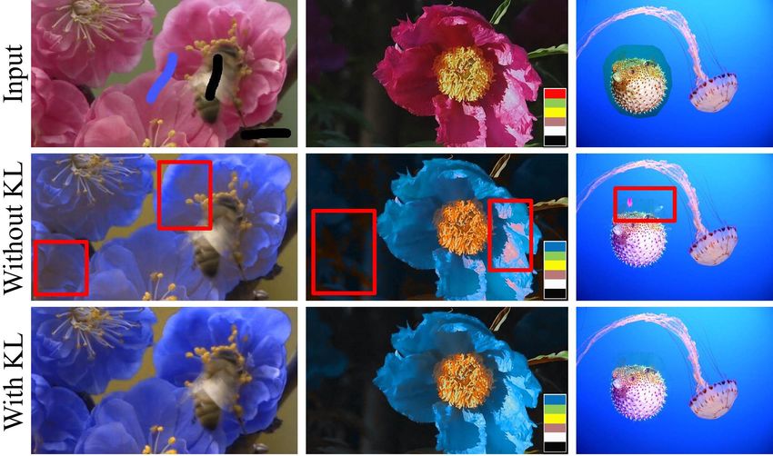
Figure 1. Sparsity-based edit propagation allows interactive recol-
applications of sparsity-based edit propagation including
oring (top), color theme editing (middle), and seamless cloning
video recoloring, theme editing, and seamless cloning, op- (bottom) with high visual fidelity. The input images (left column)
erating on both color and texture features. We demonstrate contain 39, 30, and 70 megapixels, respectively. Our edit propaga-
that with a sample-to-pixel ratio in the order of 0.01%, sig- tion is based on 70, 210, and 45 sparse samples (sample-to-pixel
nifying a significant reduction on memory consumption, our ratio of 0.01%) respectively for these three experiments.
method still maintains a high-degree of visual fidelity.
techniques also increases. Edit propagation based on global
1. Introduction optimization inevitably incurs a high cost both in memory
consumption and processing speed. For example, a naive
One of the more frequently applied operations in inter-
implementation of the method of An et al. [1] to process an
active image/video editing involves efficiently propagating
image containing 60M pixels requires about 23GB memory,
sparse user edits to an entire data domain. Edit propaga-
which exceeds the capability of many low-end commodity
tion has been a well-studied problem in computer vision
computers. A recent remedy is to rely on stochastic approx-
and it enables a variety of applications including interactive
imation algorithms [17, 27], but at the expense of lower vi-
color or tonal editing, seamless cloning, and image mat-
sual fidelity with editing artifacts.
ting. The best known edit propagation approach is affinity-
based [1, 22] and so far many variants have been developed Our key observation is that to achieve efficient and scal-
[9, 27]. Typically, the solution involves a global optimiza- able edit propagation on high-resolution images or video,
tion to propagate the edits to remaining pixels. the operations may be performed on a reduced data repre-
With the increasing availability of high-resolution im- sentation. With this in mind, we resort to sparse representa-
ages and video, the demand for scalable image processing tions for images. Research from signal processing has sug-
gested that important classes of signals such as images and
∗ corresponding author(email: lijw@vrlab.buaa.edu.cn) videos are naturally sparse with respect to fixed representa-
1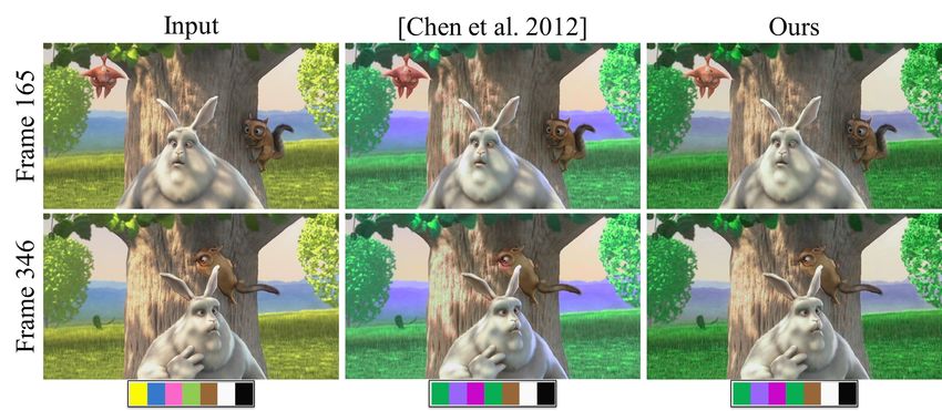
tive samples, or concatenations of such samples. That is, if        properly defined affinities between all pixels. Farbman et
a proper sample dictionary is found for an image or video, it       al. [9] employed the diffusion distance to measure affinities
suffices to edit the sparse samples instead of all pixels, thus     between pixels. However, these methods do not adequately
achieving efficiency and scalability.                               constrain pixels in blended regions, often causing halo arti-
    Using a sparse representation, instead of propagating an        facts. Chen et al. [6] addressed this problem by preserving
edit to a whole input image or video according to relation-         the manifold structure underlying the image pixels.
ships among all pixels, we compute a set of sparse, rep-                Also related are a large body of works on edge-aware
resentative samples (or features) over the image or video,          or edge-centric image processing [5, 11] and image upsam-
apply the edit to these samples only, and then propagate the        pling techniques [12]. Generally speaking, preserving affin-
edit to all pixels. Our approach follows the principles of          ity relations among all pixels is expensive, and prohibitive
sparse representations [2] and signal decorrelation using the       for high-resolution data. It is difficult for existing methods
Kullback-Leibler or KL divergence (i.e. relative entropy) to        to propagate edits with a limited time or memory budget
obtain an optimal sample set and the corresponding coding           while ensuring visual fidelity of the editing results.
coefficients for the sparse representation.                             In the past few years, various adaptations of sparse rep-
    By maximizing the KL divergence between each pair               resentations have been applied to the problem domain of
of samples in the dictionary, the cross correlation between         image analysis and understanding. Yang et al. [29] and
samples is minimized so that the set of samples is both             Allen et al. [28] used sparse representations for image
sparse and representative. These samples intrinsically cap-         super-resolution by assuming that the high-resolution image
ture a natural basis for the input data: each pixel in the input    patches have a sparse representation with respect to that of
image is represented as a linear sum over the sampled pixels        low-resolution images. Julier et al. [21] developed a super-
with the coding coefficients supplying the weights. Through         vised framework to learn multiscale sparse representations
the coding coefficients, an edit applied to the sparse samples      of color images and video for image and video denoising
can be mapped to an edit with respect to all pixels. How-           and inpainting. Yan et al. [25] proposed a semi-coupled
ever, the number of samples is far less than the number of          dictionary learning model for cross-style image synthesis.
pixels in a high-resolution image or video.                             Sparse representations have also been applied to face
    By working with the representative samples and their            recognition [26], image background modeling [3], and im-
corresponding coding coefficients for edit propagation, we          age classification [20]. More works along those lines can
leverage a representation of the input data with higher fi-         be found in a recent comprehensive survey [8]. We adopt
delity compared to Fourier or wavelet transforms [16]. By           sparse representations for edit propagation for the first time
performing the edit propagation on representative samples           and demonstrate its effectiveness in several key applications
while keeping the coding coefficients fixed, the linear rela-       when applied to high-resolution images and video.
tionship between the input data and representative samples
is preserved. In turn, this ensures that the input data is faith-   3. Sparsity-based edit propagation
fully represented by the representative samples.
    Our main contributions are: 1) an efficient edit propaga-          Given a high-resolution image, we first obtain an over-
tion method for high-resolution images or video via sparse          complete dictionary Dinit via online dictionary learning
dictionary learning; 2) an automatic scheme based on KL             [19]. Then we utilize the KL divergence (i.e. relative en-
divergence to obtain a compact and discriminative sam-              tropy) [14] as an optimization objective to turn the initial
ple set for edit propagation; 3) application of the learned         dictionary Dinit into a sparser and more representative sam-
sparse dictionary to several frequently encountered im-             ple set. An image edit is applied to the samples and propa-
age/video processing tasks including interactive recoloring,        gated from the samples to all pixels in the image.
color theme editing, and seamless cloning. We demonstrate
                                                                    3.1. Dictionary initialization
through numerous experiments that our method signifi-
cantly reduces memory cost while still maintaining high-               Let xi represent a pixel i in the input image X, where xi
fidelity editing results and avoiding the artifacts encoun-         can be a pixel color or any other editable feature, and Ninit
tered by previous methods [17, 27].                                 represent the number of samples in the overcomplete dictio-
                                                                    nary Dinit = [d1 , d2 , ..., dNinit ]. Dinit and the correspond-
2. Related work                                                     ing coefficients α for input X are obtained by minimizing
    Edit propagation is a proven and well-adopted technique                     X                       2
                                                                                    kxi − Dinit αi k2 + λ
                                                                                                              X
                                                                                                                   kαi k0 ,      (1)
for image/video editing. The work of Levin et al. [15] pro-                      i                           i
vided the first framework for propagating user edits. Later,
this work was extended by [1, 17, 27] to ensure that the ed-        where the first term gives the reconstruction error and the
its can be propagated for fragmented regions according to           l0 norm ||αi ||0 counts the number of nonzero entries in the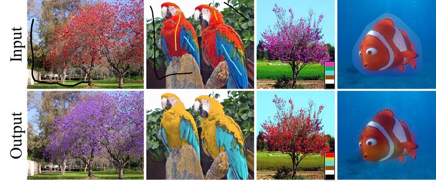
coefficient αi . Minimizing Equation (1) can be transformed       samples. Then we iteratively select the next best sample d∗
into an iterative sparse coding problem [18, 19], which can       from Dinit P\ D∗ which is the most dissimilar with D∗ , i.e.,
be solved efficiently.                                            arg maxd∗ di ∈D∗ R(d∗ , di ), adding d∗ to D∗ and remov-
                                                                  ing the samples from Dinit whose dissimilarities with d∗
3.2. Dictionary optimization                                      are less than a threshold τ , until Dinit = ∅. We use the
    The initial dictionary Dinit is overcomplete with most        threshold τ to control the compactness of D∗ .
samples redundant. A compact and discriminative dictio-              We finally update the coefficients α according to the op-
nary should capture the main information entropy of Dinit         timized sample set D∗ to obtain the corresponding coeffi-
with the chosen samples decorrelated; this essentially en-        cients α∗ for D∗ with dictionary learning [19].
courages signals having similar features to possess similar
                                                                  3.3. Edit propagation
sparse representations. We use the KL-divergence to mea-
sure the difference between two samples so as to obtain a             We use Y = [y1 , y2 , ..., yN ] to represent the correspond-
compact and discriminative sample set D∗ .                        ing edit propagation result from input X, where N de-
    In information theory, the KL-divergence is a non-            notes the number of pixels in X. We denote the result-
symmetric measure of the difference between two proba-            ing samples after edit propagation with respect to D∗ by
bility distributions P and Q,                                     D̃ = [d˜1 , d˜2 , ..., d˜n ]. Since the input image can be well rep-
                                                                resented as a linear combination of the samples D∗ and co-
             KL(P kQ) =
                           X
                               P (i) ln
                                          P (i)
                                                  .     (2)       efficients α∗ : xi ≈ D∗ αi∗ , it suffices to edit the sparse set
                            i
                                          Q(i)                    of representative samples D∗ in place of all pixels, leading
                                                                  to significant cost savings.
Although the KL-divergence is often intuited as a distance            Suppose that G represents the user edits (e.g., user scrib-
metric, it is not a true metric, e.g., due to its asymmetry. We   bles) for a subset S of pixels. We propagate the edits via
utilize a symmetrized version of KL-divergence to estimate        sparse representation by minimizing the energy,
the difference between two samples,
                                                                               arg min E = γ1 E1 + γ2 E2 + γ3 E3 ,                      (5)
         KLs (P kQ) = KL(P kQ) + KL(QkP ).                 (3)                  (d˜i ,yi )

We optimize the initial dictionary Dinit according to the         where
                                                                           X                 2      X        X
symmetric KL-divergence (3). Obviously, two similar sig-          E1 =                d˜i − gi ; E2 =   (d˜i −   wij d˜ij )2
nals in input X would use similar samples in Dinit to make               i∈S,gi ∈G                               i           d˜ij ∈Ni
the sparse decompositions. Thus the similarity between                                       X                       2
                                                                               E3 =                yi − D̃α∗i            ,
two signals can be measured by comparing the correspond-                               i,α∗    ∗
                                                                                                                     2
                                                                                          i ∈α
ing sparse coefficients. In the same way, we can estimate
the similarity of two samples in Dinit by comparing the            and Ni is a set containing the neighbors of di . The energy
number of signals using them, and their contributions in          term E1 ensures that the final representative samples are
the sparse decomposition [24]. Specifically, each sample          close to the user specified value gi . E2 seeks to maintain the
di ∈ Dinit maps all the input signals to its corresponding        relative relationship between the samples during edit propa-
row of coefficients αdi = [αi1 ...αiN ]. For each pair of sam-    gation. Chen et al. [6] proposed a manifold preserving edit
ples di and dj , we define the dissimilarity between them as      propagation method which maintains the relative relation-
R(di , dj ) = KLs (αdi kαdj ). To avoid taking logarithms of      ship between pixels by using locally linear embeddings dur-
zero, we smooth the sparse coefficients by adding a small         ing edit propagation. Here, we follow the same principle to
constant term ε = 10−16 and normalizing the distribution.         compute the local linear relationship for all representative
   Our dictionary optimization problem is therefore to find       samples. Specifically, we obtain the relationship weights
a sample set D∗ to ensure that the KL-divergence between          wij by minimizing
each sample pair in D∗ is maximized:                                                                                         2
                                                                                     n
                                                                                     X                     K
                                                                                                           X
                                                                                                 d∗i   −         wij d∗ij
                     X
          arg max           R(di , dj ), D∗ ⊆ Dinit .       (4)                                                                  ,      (6)
              D  ∗
                   di ,dj ∈D ∗                                                 i=1,d∗
                                                                                    i ∈D
                                                                                         ∗                 j=1

                                                                                              PK
Since obtaining the global optimum is difficult, we em-           subject to the constraint j=1 wij = 1, where {d∗ij |j =
ploy a greedy heuristic which resembles farthest point sam-       1, 2, ...K} are the K nearest neighbors (kNN) of d∗i .
                                     ∗
pling. Given Dinit , we start with DP  = {d0 }, where d0              Finally, the last energy term E3 is a fidelity term, which
is selected from Dinit by arg maxd0 di ∈Dinit R(d0 , di ),        constrains the final result to be faithfully represented by the
implying that it has the maximum dissimilarity with other         sparse representative samples after edit propagation.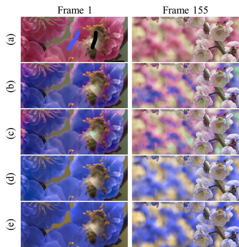
Equation (5) is a quadratic function in D̃ and Y , which      Parameters. The only two parameters to set during sam-
can be minimized by solving the two equations                    ple construction are Ninit , the number of samples in Dinit
                                                                 and the threshold τ ; the method is otherwise automatic.
(Λ1 +α∗ T Λ3 α∗ +Λ2 (I −W )T (I −W ))D̃−Λ3 α∗ Y = Λ1 G           For all experiments shown in the paper, the same param-
                                                   (7)           eter values Ninit = 500 and τ = 20 are used. Therefore,
and                                                              n ≤ Ninit = 500 is determined by the sample optimiza-
                      Y − D̃α∗        = 0,                (8)    tion progress and varies depending on the dataset processed.
                                  2                              The other parameters are also fixed: K = 10 and d = 3 for
where I is the identity matrix, Λ1 , Λ2 , and Λ3 are diagonal    RGB color features and d = 8 for texture features.
matrixes and G is a vector with
                                                                 4. Applications

              γ1     i∈S                     gi     i∈S             We now describe how to apply sparsity-based edit prop-
Λ1 (i, i) =                         Gi =
              0 otherwise                    0 otherwise         agation to various classical images and videos editing tasks.
and Λ2 (i, i) = γ2 and Λ3 (i, i) = γ3 . We set γ1 = 1000,        Video object recoloring. When a user draws scribbles
γ2 = 5, and γ3 = 1 in all our experiments. Equations (7)         with desired colors at some pixels in a frame, our method
and (8) can be solved efficiently, as shown in Algorithm (1),    only propagates the edit to the representative samples we
which gives a summary of our edit propagation scheme.            compute; see Algorithm (1). The whole video will change
                                                                 with the representative samples synchronously according to
Algorithm 1 Sparsity-based edit propagation.                     the coding coefficients, where the user-edited pixels are re-
Require: X = [x1 , ..., xN ] (input image/video)                 placed by the representative samples. Specifically, in Equa-
Ensure: Y = [y1 , ..., yN ] ≈ D̃α∗ (resulting image/video)       tion (5), we set S as the nearest colors in the dictionary
                                                                 set D∗ to that of pixels covered by the user strokes, using
 1: Calculate the initial samples Dinit from X using an on-
                                                                 the Euclidean distance in RGB space, and gi as the strokes’
    line dictionary learning method [19].
                                                                 color with black enforcing color preservation.
 2: Calculate the source representative samples D ∗ from
    Dinit using the KL-divergence method.                        Video color scheme editing. For this task, the step for
 3: Set gi in Equation (5) as the specified edits by the user    learning representative samples is the same as that for video
    according to specific applications; see Section 4.           object recoloring. Instead of specifying scribbles, the user
 4: Propagate edits across D ∗ and obtain result samples D̃.     utilizes a color theme to edit an input video or image. We
                                                                 classify the representative samples into several clusters ac-
 5: for each pixel xi of input data X do                         cording to the probabilistic mapping provided in [4], and
 6:   Calculate coefficient αi∗ of xi by Equation (1).           calculate the mean color of each cluster to generate the color
 7:   Calculate the result yi = D̃αi∗ .                          theme T of the representative samples. Then the user can
 8: end for                                                      edit T to a desired color theme R to alter the color scheme
 9: return Y (resulting image/video).                            of the whole video or image. Specifically, in Equation (5),
                                                                 we set S as the color theme T . For each color i ∈ S, gi
                                                                 denotes the corresponding color value in R.
Cost analysis. We use the online dictionary learning             Image cloning. Our edit propagation method can also be
method in [19] (line 1) for initial dictionary construction;     employed to paste a source image or video patch into an-
this scheme can manage a large dataset with low memory           other scene seamlessly. We treat image cloning as a mem-
and computational costs. In line 2, we calculate the KL-         brane interpolation problem [10]. The pixel colors along
divergence of each pair of samples in Dinit . Thus to save       the boundary of the source image constitute the source dic-
Dinit , we need a space complexity of O(Ninit d), where          tionary in our method. The target dictionary consists of the
d is the dimension of each sample (vector). In line 3, the       color differences on the boundary between the source and
user edit gi is a small part of the source representative sam-   target images. We compute the coding coefficients which
ples and does not consume additional space. The memory           can reconstruct the source image patch by the source dic-
consumption of the edit propagation in line 4 is subject to      tionary. Then we use the coding coefficients and the target
the size n of D∗ and the size K of kNN. In the for loop          dictionary to generate the membrane. By adding the mem-
from lines 5 to 8, we solve the coefficient α∗ one by one,       brane to the target image, we achieve the final cloning re-
thus the memory space used here is negligible. From the          sult. Specifically, in Equation (5), we set S as all the colors
analysis above, we can see that the space complexity of the      on the blending boundary and gi as the color differences on
algorithm is max{O(Ninit d), O(Knd)}.                            the boundary between the source and target images.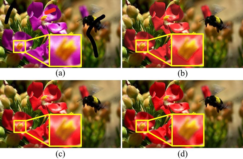
Performance comparison for video object recoloring.
Data Peony Canoeing
Resolution 30M 96M
Memory 350MB 1110MB
Xu et al.
Timing 43s 132s
Memory 825MB 2400MB
Farbman et al.
Timing 49s 141s
Memory 65MB 220MB
Chen et al.
Timing 480s 825s
Samples num. 222 210
Ours Memory 6.5MB 5.8MB
Timing 125s 425s
Table 1. Memory and timing comparison between our method and
those of [Xu et al. 2009], [Farbman et al. 2010] and [Chen et al.
2012] for object recoloring in video.
Figure 2. Video object recoloring: comparison to (b) [Xu et al.
2009], (c) [Farbman et al. 2010] and (d) [Chen et al. 2012] on two
example frames. Input video (a) “P eony” contains 30 megapixels.
[Xu et al. 2009] and [Farbman et al. 2010] generate halo artifacts
at flower boundaries. Our results (e) are more natural as well as
more efficient than [Chen et al. 2012].
5. Experimental results
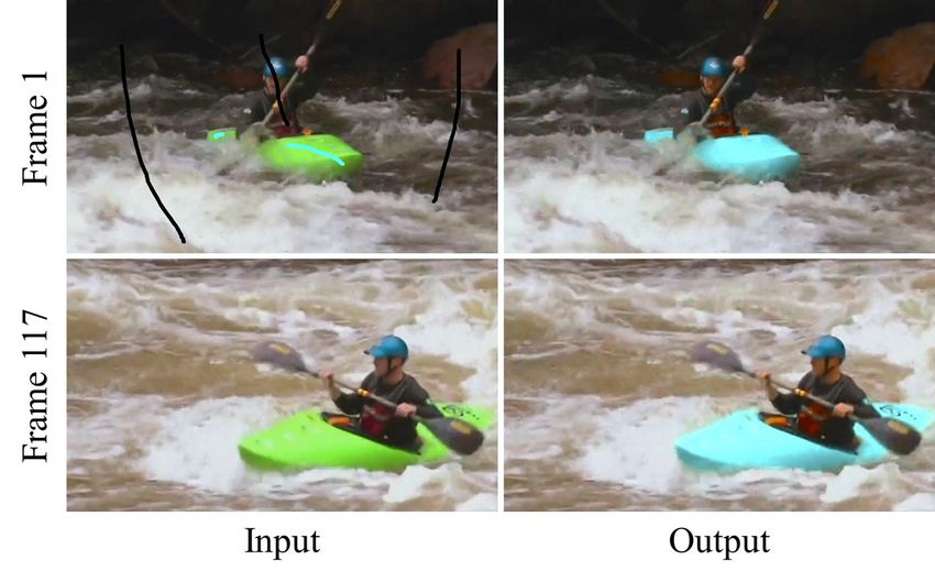
Figure 3. More visual results for video object recoloring. Shown
We demonstrate our method on applications mentioned on the left are some example frames of “Canoeing”. The right
above and compare to state-of-the-art edit propagation shows corresponding recoloring results. The video contains 96
methods such as [27, 9, 6] to show the space efficiency and megapixels. Our method only takes up 5.8MB memory space.
visual fidelity achieved by our sparsity-based approach. The
authors of these three papers kindly share their code with
around flower boundaries. In comparison, our method and
us. We also demonstrate the efficiency of our method by
the method of Chen et al. [6] produced more natural results,
operating on higher dimensional features, such as textures,
while our method incurs a much smaller memory usage; see
within our framework for video editing. Our experiments
Table 1. Specifically, for the input video “Peony” contain-
were performed on a PC with Intel Core i7 Quad processor
ing 30M pixels, our method takes 6.5MB RAM, while Xu
(3.40GHz, 8 cores) and 4 GB memory.
et al. [27], Farbman et al. [9] and Chen et al. [6] required
Due to space limitations, we are only able to show se- 350MB, 825MB, and 65MB RAM, respectively.
lected results in the paper for a demonstration. We would Figure 3 shows a result for high-resolution video se-
like to point out that these results are representative of the quences. The input video “Canoeing” contains 96M pixels.
efficiency and advantages that our method would offer, in We use only 210 samples in our sparsity-based edit propa-
comparison to previous state-of-the-art approaches. More gation, resulting in only 5.8MB RAM usage. The running
results can be found in the supplementary material. time for this example is 425 seconds.
Object recoloring in video. Figure 2 shows a compari- Video color theme editing. Figure 4 shows a comparison
son, where results from competing methods were obtained with the method of Chen et al. [6] on color theme editing.
under suggested parameter settings in the original papers The input video “Big Bunny” has 468 frames whose reso-
[27, 9, 6]. The user applied strokes to one frame of the video lution is 1920×1080; it contains 970M pixels in total. We
to change the red flowers to blue. One can see that the fore- compute 240 sparse representative samples automatically
ground flowers are not edited appropriately in the results of for edit propagation. Visually, we can obtain similar results
Xu et al. [27] and Farbman et al. [9]: halo artifacts appear with the method of [6]. However, our method takes 8MB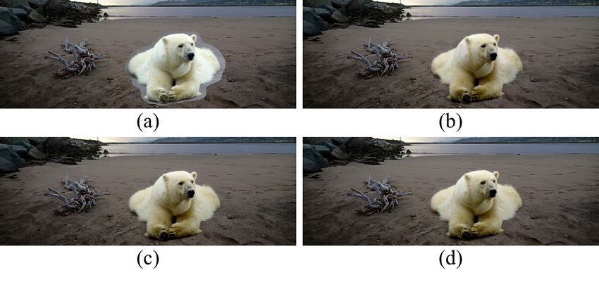
Figure 4. Comparison with [Chen et al. 2012] on color theme            Figure 7. Visual results for video cloning. The first row shows the
editing. The first column contains sample frames from the orig-        composited result without blending after scaling the input objects
inal video “BigBunny”. The next two columns are results from           while the second row is the blending result with our method.
[Chen et al. 2012] and our method, respectively.
                                                                             Comparison for video color theme editing.
                                                                                          Data        Daisy Big Bunny
                                                                                        Resolution     30M       970M
                                                                                         Memory       80MB     1000MB
                                                                           Chen et al.
                                                                                         Timing        650s      3200s
                                                                                       Samples num.     212       240
                                                                             Ours        Memory        6MB       8MB
                                                                                         Timing        212s       630s
                                                                       Table 2. Memory and timing comparison between our method and
                                                                       [Chen et al. 2012] for video color theme editing.

Figure 5. Results on video color theme editing. Shown on the left
are some example frames of the video “Daisy”. Right are the
corresponding recolored results.
                                                                       Figure 8. Edit propagation results with and without texture fea-
                                                                       tures. (a) input image; (b) edit result with only color features; (c)
                                                                       result with additional texture features. Our method automatically
                                                                       selects 165 samples from the input to arrive at the result (c).

                                                                       for seamless cloning, we find all three results to be visu-
                                                                       ally pleasing and almost indistinguishable. However, our
                                                                       method only uses 107 samples, translating to a 3MB mem-
                                                                       ory footprint, for the shown example, which is a lot more
                                                                       memory efficient than the other methods. Figure 7 shows
Figure 6. Comparison with previous cloning methods. (a) is the
                                                                       our results for video cloning. A video clip of a jellyfish was
composited image and (b) is our result; (c) and (d) were obtained
by [Pérez et al. 2003] and [Farbman et al. 2009], respectively. The
                                                                       blended into another video as shown in the first row. The
three results are visually indistinguishable.                          second row shows the blended results. Our method achieves
                                                                       temporally consistent video blending by using only 45 sam-
                                                                       ples and the task was executed in180 seconds.
memory space for the task while Chen et al. [6] consumes
about 1,000MB RAM; see Table 2.                                        Texture features. Our method is applicable to higher di-
   Figure 5 shows another result from video color theme                mensional features such as textures, as shown in Figure 8.
editing. The target video “Daisy” contains 129 frames and              We calculate the texture features for the input by using the
30M pixels. Our method takes up 6MB RAM and 212 sec-                   method in [7]. It is easy to detect that the input image (a)
onds to propagate the edits to the whole video.                        contains two different textures with only one color. Editing
                                                                       based on color features only would lead to the result in (b)
Image cloning. Figure 6 compares one of our image                      in which all regions are recolored to red, while these regions
cloning results to Pérez et al. [23] and Farbman et al. [10].         exhibit two distinctive texture patterns. Figure 8(c) shows
While it is difficult to provide a quantitative evaluation             the importance of taking into account texture features. Our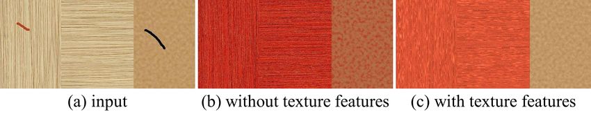
Figure 10. Comparison between using KL divergence and using
                                                                     maximum mutual information (MMI) for images editing. Note
                                                                     the artifacts with the use of MMI.

Figure 9. Comparison between using and without using KL-
divergence in sample construction. The three columns from left to
right: objects recoloring, color theme editing, and image cloning.
Artifacts appear when KL-divergence optimization was not ap-
plied, while the counterpart produces more natural results.

method automatically selected 165 samples, requiring only
11MB memory, for this shown example.

Test on KL-divergence. Figure 9 shows a comparison
between results obtained using vs. without using KL-
divergence in representative sample construction, for all
three applications. Our method automatically selects 222,
210, and 160 samples for these three applications, respec-           Figure 11. Varying the number of representative samples. (a) input
tively. It is evident that with the same number of samples,          image; (b) 50 samples — too few with small artifacts near the blos-
the KL-divergence based scheme achieves better results.              som (see inset); (c) 70 samples using KL-divergence — adequate.
   We tested our method on 1,053 images to evaluate the              (d) 80 samples — more samples do not improve results.
reconstruction error, which is computed using Sum of Ab-
solute Differences. With KL divergence optimization, the
error is 0.0073, while for the method of Mairal et al. [19]
without sample optimization, the error is at 0.0111.
   We also compared KL divergence against Maximum
Mutual Information (MMI) [13], a well-known information
entropy theory, in sample selection for reconstruction and
edit propagation. As shown in Figure 10, given the same
number of initial samples, our method generated a natural
editing result while artifacts emerged in the result produced        Figure 12. Several editing results on consumer video or photos.
with MMI. This demonstrates that the use of KL-divergence
tends to capture more representative samples than other al-
ternatives of information entropy, such as MMI.                         Finally, we show a few editing results obtained on con-
                                                                     sumer video or photos to further demonstrate our method
Varying size of sample set. We evaluate our method in                on complex image data, as shown in Figure 12.
Figure 11 with different number of representative samples.
Desirably, the number of representative samples should be            6. Conclusion and discussion
just large enough to best represent the input data. For this
example, our method automatically selected 70 samples and               We develop a novel sparsity-based edit propagation
the result shown in (c) is natural. If we randomly eliminate         method for high-resolution images or video. Instead of
20 samples from the representative set, the propagation re-          propagating an edit to the whole image or video accord-
sult exhibits artifacts along the boundary of the blossom,           ing to relationships among all pixels, by using sparse dic-
as shown in (b). On the other hand, the propagation result           tionary learning, we derive a set of representative samples
does not improve if we add more samples from the initial             (or features), apply the edit to these samples only, and then
dictionary, as shown in (d).                                         propagate. Our method significantly improves the memory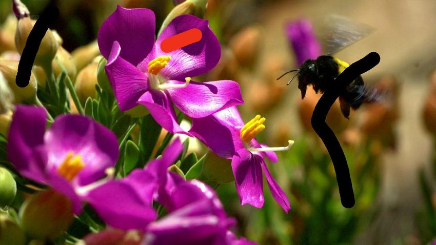
efficiency while maintaining a high-degree of visual fidelity        [11] R. Fattal, R. Carroll, and M. Agrawala. Edge-based image
in the editing results. Several frequently encountered appli-             coarsening. ACM Trans. Graph., 29(1), 2009. 2
cations enabled by our proposed method, including interac-           [12] J. Kopf, M. F. Cohen, D. Lischinski, and M. Uyttendaele.
tive image/video recoloring, color theme editing, and image               Joint bilateral upsampling. ACM Trans. Graph., 26(3), July
cloning, demonstrate the effectiveness of our approach.                   2007. 2
    One limitation of our current method is that it is not de-       [13] A. Krause, A. Singh, and C. Guestrin. Near-optimal sen-
signed to alter only one object: if two far away objects in               sor placements in gaussian processes: Theory, efficient algo-
an image share the same features, editing one object would                rithms and empirical studies. J. Mach. Learn. Res., 9:235–
change the other. As Figure 11 shows, two flowers are re-                 284, June 2008. 7
colored into red even if only one is scribbled by the user. Al-      [14] S. Kullback and R. A. Leibler. On information and suffi-
though some video cutout methods can be applied as a rem-                 ciency. Ann. Math. Statist., 22(1):79–86, 1951. 2
edy, it is labor-intensive and time-consuming for users to           [15] A. Levin, D. Lischinski, and Y. Weiss. Colorization using
perform additional operations. For future work, we would                  optimization. ACM Trans. Graph., 23(3), 2004. 2
like to incorporate spatial information for edit propagation         [16] M. S. Lewicki and T. J. Sejnowski. Learning overcomplete
and investigate further means of optimization, e.g., by em-               representations. Neural Comput., 12(2):337–365, 2000. 2
ploying GPU processing, to improve efficiency.                       [17] Y. Li, T. Ju, and S.-M. Hu. Instant propagation of sparse edits
                                                                          on images and videos. Comput. Graph. Forum, 29(7):2049–
Acknowledgement. We thank the reviewers for their                         2054, 2010. 1, 2
valuable feedback. This work is supported in part by grants          [18] J. Mairal, F. Bach, and J. Ponce. Task-driven dictio-
from NSFC (61325011), 863 program (2013AA013801),                         nary learning. IEEE Trans. Pattern Anal. Mach. Intell.,
SRFDP (20131102130002), BUAA (YWF-13-A01-027),                            34(4):791–804, 2012. 3
and NSERC (611370).                                                  [19] J. Mairal, F. Bach, J. Ponce, and G. Sapiro. Online learning
                                                                          for matrix factorization and sparse coding. J. Mach. Learn.
References                                                                Res., 11:19–60, Mar. 2010. 2, 3, 4, 7
                                                                     [20] J. Mairal, F. Bach, J. Ponce, G. Sapiro, and A. Zisserman.
 [1] X. An and F. Pellacini. Appprop: all-pairs appearance-
                                                                          Discriminative learned dictionaries for local image analysis.
     space edit propagation. ACM Trans. Graph., 27(3):40:1–
                                                                          In CVPR, pages 1–8, 2008. 2
     40:9, Aug. 2008. 1, 2
 [2] A. M. Bruckstein, D. L. Donoho, and M. Elad. From sparse        [21] J. Mairal, G. Sapiro, and M. Elad. Learning multiscale sparse
     solutions of systems of equations to sparse modeling of sig-         representations for image and video restoration. Multiscale
     nals and images. SIAM Rev., 51(1):34–81, Feb. 2009. 2                Modeling & Simulation, 7(1):214–241, 2008. 2
 [3] V. Cevher, A. Sankaranarayanan, M. F. Duarte, D. Reddy,         [22] F. Pellacini and J. Lawrence. Appwand: editing measured
     R. G. Baraniuk, and R. Chellappa. Compressive sensing                materials using appearance-driven optimization. ACM Trans.
     for background subtraction. In Proc. ECCV, pages 155–168,            Graph., 26(3), 2007. 1
     Berlin, Heidelberg, 2008. 2                                     [23] P. Pérez, M. Gangnet, and A. Blake. Poisson image editing.
 [4] Y. Chang, S. Saito, and M. Nakajima. A framework for trans-          ACM Trans. Graph., 22(3):313–318, 2003. 6
     fer colors based on the basic color categories. In Proc. of     [24] I. Ramirez, P. Sprechmann, and G. Sapiro. Classification
     Computer Graphics International, pages 176–183, 2003. 4              and clustering via dictionary learning with structured inco-
 [5] J. Chen, S. Paris, and F. Durand. Real-time edge-aware im-           herence and shared features. In CVPR, pages 3501–3508,
     age processing with the bilateral grid. ACM Trans. Graph.,           2010. 3
     26(3), 2007. 2                                                  [25] S. Wang, L. Zhang, L. Y., and Q. Pan. Semi-coupled dic-
 [6] X. Chen, D. Zou, Q. Zhao, and P. Tan. Manifold preserving            tionary learning with applications in image super-resolution
     edit propagation. ACM Trans. Graph., 31(6):132:1–132:7,              and photo-sketch synthesis. In Proc. CVPR, 2012. 2
     Nov. 2012. 2, 3, 5, 6
                                                                     [26] J. Wright, A. Y. Yang, A. Ganesh, S. S. Sastry, and Y. Ma.
 [7] J. G. Daugman. Uncertainty relation for resolution in
                                                                          Robust face recognition via sparse representation. IEEE
     space, spatial frequency, and orientation optimized by two-
                                                                          Trans. Pattern Anal. Mach. Intell., 31(2):210–227, 2009. 2
     dimensional visual cortical filters. Optical Society of Amer-
     ica A, 2(7):1160–1169, 1985. 6                                  [27] K. Xu, Y. Li, T. Ju, S.-M. Hu, and T.-Q. Liu. Efficient
                                                                          affinity-based edit propagation using k-d tree. ACM Trans.
 [8] M. Elad, M. A. T. Figueiredo, and Y. Ma. On the Role of
                                                                          Graph., 28(5), 2009. 1, 2, 5
     Sparse and Redundant Representations in Image Processing.
     Proc. the IEEE, 98(6):972 –982, 2010. 2                         [28] A. Y. Yang, J. Wright, Y. Ma, and S. S. Sastry. Unsupervised
 [9] Z. Farbman, R. Fattal, and D. Lischinski. Diffusion maps for         segmentation of natural images via lossy data compression.
     edge-aware image editing. ACM Trans. Graph., 29(6), 2010.            Comput. Vis. Image Und., 110(2):212–225, 2008. 2
     1, 2, 5                                                         [29] J. Yang, J. Wright, T. S. Huang, and Y. Ma. Image super-
[10] Z. Farbman, G. Hoffer, Y. Lipman, D. Cohen-Or, and                   resolution via sparse representation. Trans. Img. Proc.,
     D. Lischinski. Coordinates for instant image cloning. ACM            19(11):2861–2873, Nov. 2010. 2
     Trans. Graph., 28(3), 2009. 4, 6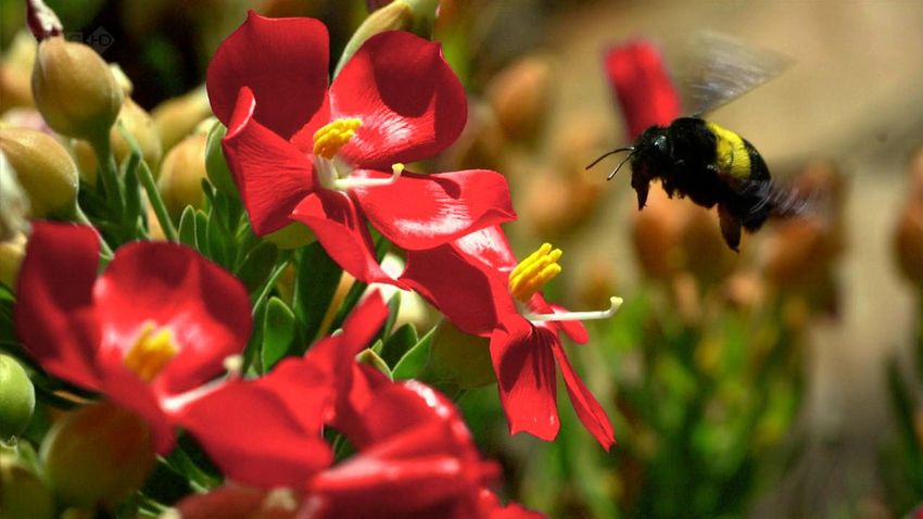
You can also read