LEARNING EFFICIENT PLANNING-BASED REWARDS FOR IMITATION LEARNING

Under review as a conference paper at ICLR 2021

L EARNING E FFICIENT P LANNING - BASED R EWARDS
FOR I MITATION L EARNING

 Anonymous authors
 Paper under double-blind review

 A BSTRACT

 Imitation learning from limited demonstrations is challenging. Most inverse rein-
 forcement learning (IRL) methods are unable to perform as good as the demon-
 strator, especially in a high-dimensional environment, e.g, the Atari domain. To
 address this challenge, we propose a novel reward learning method, which stream-
 lines a differential planning module with dynamics modeling. Our method learns
 useful planning computations with a meaningful reward function that focuses on
 the resulting region of an agent executing an action. Such a planning-based reward
 function leads to policies with better generalization ability. Empirical results with
 multiple network architectures and reward instances show that our method can
 outperform state-of-the-art IRL methods on multiple Atari games and continuous
 control tasks. Our method achieves performance that is averagely 1,139.1% of the
 demonstration.

1 I NTRODUCTION

Imitation learning (IL) offers an alternative to reinforcement learning (RL) for training an agent,
which mimics the demonstrations of an expert and avoids manually designed reward functions.
Behavioral cloning (BC) (Pomerleau, 1991) is the simplest form of imitation learning, which learns a
policy using supervised learning. More advanced methods, inverse reinforcement learning (IRL) (Ng
& Russell, 2000; Abbeel & Ng, 2004) seeks to recover a reward function from the demonstrations
and train an RL agent on the recovered reward function. In the maximum entropy variant of IRL, the
aim is to find a reward function that makes the demonstrations appear near-optimal on the principle
of maximum entropy (Ziebart et al., 2008; 2010; Boularias et al., 2011; Finn et al., 2016).
However, most state-of-the-art IRL methods fail to meet the performance of demonstrations in high-
dimensional environments with limited demonstration data, e.g., a one-life demonstration in Atari
domain (Yu et al., 2020). This is due to the main goal of these IRL approaches is to recover a reward
function that justifies the demonstrations only. The rewards recovered from limited demonstration
data would be vulnerable to the overfitting problem. Optimizing these rewards from an arbitrary
initial policy results in inferior performance. Recently, Yu et al. (2020) proposed generative intrinsic
reward learning for imitation learning with limited demonstration data. This method outperforms
expert and IRL methods in several Atari games. Although GIRIL uses the prediction error as curiosity
to design the surrogate reward that encourages (pushes) states away from the demonstration and
avoids overfitting, the curiosity also results in ambiguous quality of the rewards in the environment.
In this paper, we focus on addressing the two key issues of previous methods when learning with
limited demonstration data, i.e., 1) overfitting problem, and 2) ambiguous quality of the reward
function. To address these issues, we propose to learn a straightforward surrogate reward function by
learning to plan from the demonstration data, which is more reasonable than the previous intrinsic
reward function (i.e., the prediction error between states). Differential planning modules (DPM) is
potentially useful to achieve this goal, since it learns to map observation to a planning computation for
a task, and generates action predictions based on the resulting plan (Tamar et al., 2016; Nardelli et al.,
2019; Zhang et al., 2020). Value iteration networks (VIN) (Tamar et al., 2016) is the representative
one, which represents value iteration as a convolutional neural network (CNN). Meaningful reward
and value maps have been learned along with the useful planning computation, which leads to policies
that generalize well to new tasks. However, due to the inefficiency of summarizing complicated
transition dynamics, VIN fails to scale up to the Atari domain.

 1

Under review as a conference paper at ICLR 2021

To address this challenge, we propose a novel method called variational planning-embedded reward
learning (vPERL), which is composed of two submodules: a planning-embedded action back-tracing
module and the transition dynamics module. We leverage a variational objective based on the
conditional variational autoencoder (VAE) (Sohn et al., 2015) to jointly optimize the two submodules,
which greatly improves the generalization ability. This is critical for the success of achieving a
straightforward and smooth reward function and value function with limited demonstration data.
As shown in Figure 1, vPERL learns meaningful reward and value maps that attends to the resulting
region of the agent executing an action, which indicates meaningful planning computation. However,
directly applying VIN in Atari domain in the way of supervised learning (Tamar et al., 2016) only
learns reward and value maps that attend no specific region, which usually results in no avail.

 (a) State. (b) vPERL Reward and Value Maps. (c) VIN Reward and Value Maps.

Figure 1: Visualization of state, reward and value maps of vPERL and VIN on Battle Zone game (the
first row) and Breakout game (the second row).

Empirical results show that our method outperforms state-of-the-art IRL methods on multiple Atari
games and continuous control tasks. Remarkably, our methods achieve performance that is up to
58 times of the demonstration. Moreover, the average performance improvement of our method is
1,139.1% of the demonstration over eight Atari games.

2 BACKGROUND AND R ELATED L ITERATURE

Markov Decision Process (MDP)(Bellman, 1966) is a standard model for sequential decision
making and planning. An MDP M is defined by a tuple (S, A, T, R, γ), where S is the set of states,
A is the set of actions, T : S × A × S → R+ is the environment transition distribution, R : S → R
is the reward function, and γ ∈ (0, 1) is the discount factor (Puterman, 2014). The expected
discounted return or value of the policy π is given by V π (s) = Eτ [ t=0 γ t R(st , at )|s0 = s], where
 P
τ = (s0 , a0 , s1 , a1 , · · · ) denotes the trajectory, in which the actions are selected according to π,
s0 ∼ T0 (s0 ), at ∼ π(at |st ), and st+1 ∼ T (st+1 |st , at ). The goal in an MDP is to find the optimal
policy π ∗ that enables the agent to obtain high long-term rewards.
Generative Adversarial Imitation Learning (GAIL) (Ho & Ermon, 2016) extends IRL by inte-
grating adversarial training technique for distribution matching (Goodfellow et al., 2014). GAIL
performs well in low-dimensional applications, e.g., MuJoCo. However, it does not scale well to
high-dimensional scenarios, such as Atari games (Brown et al., 2019a). Variational adversarial
imitation learning (VAIL) (Peng et al., 2019) improves on GAIL by compressing the information
via variational information bottleneck. GAIL and VAIL inherit problems of adversarial training, such
as instability in training process, and are vulnerable to overfitting problem when learning with limited
demonstration data. We have included both methods as comparisons to vPERL in our experiments.
Generative Intrinsic Reward driven Imitation Learning (GIRIL) (Yu et al., 2020) leverage gen-
erative model to learn generative intrinsic rewards for better exploration. Though GIRIL outperforms
previous IRL methods on several Atari games, the reward map of GIRIL is ambiguous and less
informative, which results in inconsistent performance improvements in different environments.
In contrast, our vPERL learns efficient planning-based reward that is more straightforward and
informative. We have included GIRIL as a competitive baseline in our experiments.
Differentiable planning modules perform end-to-end learning of planning computation, which
leads to policies that generalize to new tasks. Value iteration (VI) (Bellman, 1957) is a well-known
method for calculating the optimal value V ∗ and optimal policy π ∗ : Vn+1 (s) = maxa Qn (s, a),

 2

Under review as a conference paper at ICLR 2021

where Qn (s, a) = R(s, a) + γ s0 T (s0 |s, a)Vn (s0 ) denotes the Q value in the nth iteration. The
 P
value function Vn in VI converges as n → ∞ to V ∗ , from which the optimal policy may be derived
as π ∗ (s) = arg maxa Q∞ (s, a).
Value iteration networks (VIN) (Tamar et al., 2016) proposes to embed value iteration (VI) (Bellman,
1957) process with a recurrent convolutional network, and generalizes well in conventional navigation
domains. VIN assumes there is some unknown embedded MDP M where the optimal plan in M
contains useful information about the optimal plan in the original MDP M . VIN connects the
two MDPs with a parametric reward function R = fR (s). Nardelli et al. (2019) proposes value
propagation networks (VPN) generalize VIN for better sample complexity by employing value
propagation (VProp). Recently, universal value iteration networks (UVIN) extends VIN to spatially
variant MDPs (Zhang et al., 2020). Although VIN can be extended to irregular spatial graphs by
applying graph convolutional operator (Niu et al., 2018), most of the VIN variants still focus on
solving the conventional navigation problems (Zhang et al., 2020).
In this paper, we extend differentiable planning module to learn an efficient reward function for
imitation learning on limited demonstration data. We dig more on leveraging the learned reward
function for imitation learning; while previous related work of VIN focuses more on the value
function. Therefore, our work is complementary to the research of VIN and its variants. Note that
any differentiable planning module can be embedded in our method. As a simple example, we utilize
the basic VIN as a backbone to build our reward learning module.

3 VARIATIONAL P LANNING - EMBEDDED R EWARD L EARNING
In this section, we introduce our solution, variational planning-embedded reward learning (vPERL).
As illustrated in Figure 2, our reward learning module is composed of two submodules to accomplish
planning-embedded action back-tracing and explicit forward transition dynamics modeling.

 K recurrence
 vPERL
 Prev. Value
 New Value
 
 ത ത
 ത ∗
 ത ത

 Action Back-tracing 

 +1 

 Transition Modeling ′ ′
 Prev. Value
 ഥ
 ′ ഥ∗
 ′
 ഥ
 ′
 ′ ഥ
 ′ ഥ
 ′
 New Value

 K recurrence

 Figure 2: Illustration of the proposed vPERL model.

3.1 ACTION BACK - TRACING AND F ORWARD DYNAMICS M ODELLING IN V PERL

Planning-embedded action back-tracing. Instead of directly applying VIN for policy learning
(Tamar et al., 2016), we build our first submodule qφ (at |st , st+1 ) for action back-tracing. As
illustrated in the top section of Figure 2, we first obtain the reward map R = fR (st , st+1 ) on an
embedded MDP M , where fR is a convolutional layer. A VI module fV I takes in the reward map
R, and effectively performs K times of VI by recurrently applying a convolutional layer Q for
K times (Tamar et al., 2016). The Q layer is then max-pooled to obtain the next-iteration value
V . The right-directed circular arrow in a light-blue color denotes the direction of convolutions.
 ∗
Then, we simply obtain the action from the intermediate optimal value V by an action mapping
 ∗
function: at = fa (V ). On these terms, we build our planning-embedded action back-tracing
submodule, which is formally represented as qφ (at |st , st+1 ) = fa (fV I (fR (st , st+1 ))). Since the

 3

Under review as a conference paper at ICLR 2021

convolutional kernel is incapable of summarizing the transition dynamics in a complex environment,
directly training this submodule is still insufficient for learning efficient reward function and planning
computation in an environment like Atari domain.
Explicit transition dynamics modeling via inverse VI. To address this, we further build upon
another submodule pθ (st+1 |at , st ) for explicit transition dynamics modeling. We build the submodule
based on the inverse VI module, which is a NN architecture that mimics the process of the inverse
version of VI. The implementation of the inverse VI module is straightforward. We first map the
action for the intermediate optima value in another embedded MDP M 0 by a value mapping function:
 ∗
V 0 = fV 0 (st , at ). Then, we apply the inverse VI module to obtain the reward map R0 . The inverse
VI module fV0 I takes in the intermediate value V 0 and recurrently apply a deconvolutional layer
Q0 for K times on the value to obtain the reward map R0 . The left-directed circular arrow in a
purple color denotes the direction of deconvolutions. To accomplish the transition, we map the
obtained R0 to the future state by: st+1 = fs0 (R0 ). The transition modeling is therefore presented
as pθ (st+1 |at , st ) = fs0 (fV0 I (fV 0 (st , at ))), which is a differentiable submodule, and can be trained
simultaneously with the action back-tracing submodule.
Variational solution to vPERL. A variational autoencoder (VAE) (Kingma & Welling, 2013) can
be defined as being an autoencoder whose training is regularised to avoid overfitting and ensure that
the latent space has good properties that enable generative process. To avoid the learned planning-
based reward overfitting to the demonstration, we optimize both submodules in a unified variational
solution, which follows the formulation of conditional VAE (Sohn et al., 2015). Conditional VAE
is a conditional generative model for structured output prediction using Gaussian latent variables,
which is composed of a conditional encoder, decoder and prior. Accordingly, we regard the action
back-tracing module qφ (z|st , st+1 ) as the encoder, pθ (st+1 |z, st ) as the decoder, and pθ (z|st ) as the
prior. Our vPERL module is maximized with the following objective:
 L(st , st+1 ; θ, φ) = Eqφ (z|st ,st+1 ) [log pθ (st+1 |z, st )] − KL(qφ (z|st , st+1 )kpθ (z|st ))
 (1)
 − αKL(qφ (ât |st , st+1 )kπE (at |st ))]
where z is the latent variable, πE (at |st ) is the expert policy distribution, ât = Softmax(z) is the
transformed latent variable, α is a positive scaling weight. The first two terms on the RHS of Eq. (1)
in the first line denote the evidence lower bound (ELBO) of the conditional VAE (Sohn et al., 2015).
These two terms are critical for our reward learning module to perform planning-based action back-
tracing and transition modeling. Additionally, we integrate the third term on the RHS of Eq. (1) in
the second line to further boost the action back-tracing. The third term minimizes the KL divergence
between the expert policy distribution πE (at |st ) and the action distribution qφ (ât |st , st+1 ), where
ât = Softmax(z) is transformed from the latent variable z. In this way, we train the forward state
transition and action back-tracing simultaneously.

Algorithm 1 Imitation learning via variational planning-embedded reward learning (vPERL).
 1: Input: Expert demonstration data D = {(si , ai )}Ni=1 .
 2: Initialize policy π, and the dual planning networks.
 3: for e = 1, · · · , E do
 4: Sample a batch of demonstration D̃ ∼ D.
 5: Train vPERL module on D̃ to converge.
 6: end for
 7: for i = 1, · · · , MAXITER do
 8: Update policy via any policy gradient method, e.g., PPO on the learned surrogate reward rt .
 9: end for
10: Output: Policy π.

Note that the full objective in Eq. (1) is still a variational lower bound of the marginal likelihood
log(pθ (st+1 |st )). Accordingly, it is reasonable to maximize this as an objective of our reward learning
module. By optimizing the objective, we improve the forward state transition and action back-tracing.
As a result, our reward learning module efficiently models the transition dynamics of the environment.
During training, we use the latent variable z as the intermediate action. After training, we will
calculate the surrogate rewards from the learned reward map. As shown in Figure 1, our method
learns meaningful reward map, which highlights the resulting region of an agent executing one action.

 4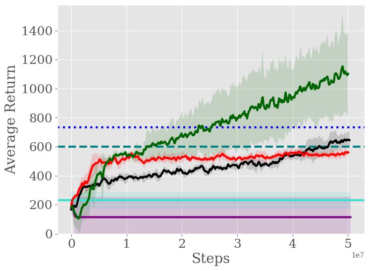

Under review as a conference paper at ICLR 2021

To leverage such meaningful information, we calculate two types of rewards that both correspond
to the highlighted informative region, i.e., rt = RMax = max R and rt = RMean = meanR, which
uses the maximum and mean value of the reward map R, respectively.
Algorithm 1 summarizes the full training procedure of imitation learning via vPERL. The process
begins by training a vPERL module for E epochs (steps 3-6). In each training epoch, we sample a
mini-batch demonstration data D̃ with a mini-batch size of B and maximize the objective in Eq. (1).
Then in steps 7-9, we update the policy π via any policy gradient method, e.g., PPO (Schulman et al.,
2017), so as to optimize the policy π with the learned surrogate reward function rt .

4 E XPERIMENTS

4.1 ATARI G AMES

We first evaluate our proposed vPERL on one-life demonstration data for eight Atari games within
OpenAI Gym (Brockman et al., 2016). To enable a fair comparison, we evaluate our method and
all other baselines under the same standard setup, where we train an agent to play Atari games
without access to the true reward function (Ibarz et al., 2018; Brown et al., 2019a). The games and
demonstration details are provided in Table 1.
A one-life demonstration only contains the
states and actions performed by an expert player
until they lose their life in a game for the first Table 1: Statistics of Atari environments.
time (Yu et al., 2020). In contrast, one full- Demonstration Length # Lives
episode demonstration contains states and ac-
 Game One-life Full-episode available
tions after the expert player loses all available
lives in a game. Therefore, the one-life demon- Kung-Fu Master 1,167 3,421 4
 Battle Zone 260 1,738 5
stration data is much more limited than one full- Centipede 166 663 3
episode demonstration. We define three levels Seaquest 562 2,252 4
of performance: 1) basic one-life demonstration- Q*bert 787 1,881 4
level - gameplay up to one life lost (“one-life"), Breakout 1,577 2,301 5
 Beam Rider 1,875 4,587 3
2) expert-level - gameplay up to all-lives lost Space Invaders 697 750 3
(“one full-episode"), and 3) beyond expert -
“better-than-expert" performance.
Our ultimate goal is to train an imitation agent that can achieve a better-than-expert performance with
the demonstration data recorded up to the moment of losing their first life in the game.
Demonstrations To generate one-life demonstrations, we trained a PPO (Schulman et al., 2017)
agent with the ground-truth reward for 10 million simulation steps. We used PPO implementation
with the default hyper-parameters in the repository (Kostrikov, 2018). As Table 1 shows, the one-life
demonstrations are all much shorter than the full-episode demonstrations, which make for extremely
limited training data.
Experimental Setup Our first step was to train a reward learning module for each game on the one-
life demonstration. We set K = 10 in vPERL for all of the Atari games. By default, we use a neural
network architecture that keeps the size of the reward map and value maps the same as that of the state,
which is 84 × 84. We achieve this by using a convolutional kernel of size 3 for each convolutional
layer, and applying padding. The corresponding method is called ‘vPERL-Large’. Additionally,
to enable faster learning, we implement our method with another neural network architecture that
reduces the size of the reward map and value maps into 18 × 18. The corresponding method is called
‘vPERL-Small’. Both vPERL-Large and vPERL-Small can learn meaningful reward map as well
as useful planning computation. Training was conducted with the Adam optimizer (Kingma & Ba,
2015) at a learning rate of 3e-5 and a mini-batch size of 32 for 50,000 epochs. In each training epoch,
we sampled a mini-batch of data every four states.
To evaluate the quality of our learned reward, we trained a policy to maximize the inferred reward
function via PPO. We set α = 100 for training our reward learning module. We trained the PPO on
the learned reward function for 50 million simulation steps to obtain our final policy. The PPO is
trained with a learning rate of 2.5e-4, a discount factor of 0.99, a clipping threshold of 0.1, an entropy
coefficient of 0.01, a value function coefficient of 0.5, and a GAE parameter of 0.95 (Schulman et al.,

 5

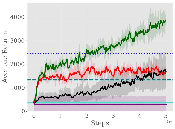
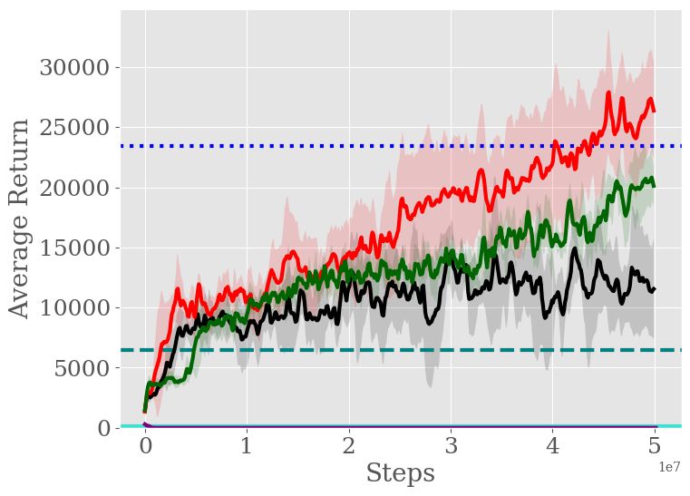
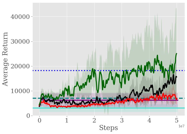
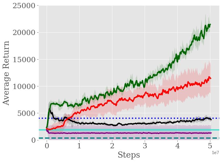
Under review as a conference paper at ICLR 2021

2016). We compared imitation performance by our vPERL agent against VIN, two state-of-the-art
inverse reinforcement learning methods, GAIL (Ho & Ermon, 2016) and VAIL (Peng et al., 2019).
More details of setup are outlined in Appendix F.2.
Results In Figure 3, we report
the performance by normalizing
the demonstration performance to
1. Figure 3 shows that vPERL
achieves performance that is usu-
ally close or better than that of the
expert demonstrator. The most im-
pressive one is the Centipede game,
our vPERL achieves performance
that is around 60 times higher than
the demonstration. GIRIL achieves
the second best performance in
Centipede, beating the demonstra-
tion by around 30 times. On the
Qbert game, vPERL beats all other
baselines by a large margin, achiev-
ing performance that is more than Figure 3: Performance improvement of vPERL and baselines.
15 times of the demonstration.

Table 2: Average return of vPERL with two types network architectures (Large and Small) and
two types of rewards (RMax and RMean ), GIRIL (Yu et al., 2020), VIN and state-of-the-art IRL
algorithms GAIL (Ho & Ermon, 2016) and VAIL (Peng et al., 2019) with one-life demonstration
data on eight Atari games. The results shown are the mean performance over five random seeds
with better-than-expert performance in bold. The last two rows show the average performance
improvements of IL algorithms versus demonstration (Demo.) and expert performance with greater
than 100% in bold.
 Expert Demo. PPO-50M vPERL-Large vPERL-Small Imitation Learning Algorithms
 Game Average Average Average RMax RMean RMax RMean GIRIL VAIL GAIL VIN
 Kung-Fu Master 23,434.8 6,500.0 38,580.0 20,700.0 18,900.0 20,800.0 20,518.3 26,742.6 11,751.2 1.3 190.4
 Battle Zone 18,137.5 7,000.0 33,400.0 27,500.0 11,000.0 47,200.0 21,899.1 7,372.8 14,222.7 6,200.0 3,372.0
 Centipede 4,069.4 360.0 7,704.6 15,516.9 10,448.8 17,371.4 21,113.4 11,446.5 3,936.1 1,306.5 1,907.6
 Seaquest 1,744.5 440.0 1,920.0 706.0 756.0 816.0 1,634.2 624.8 476.1 60.0 148.0
 Q*bert 13,441.5 8,150.0 26,235.0 71,920.0 165,325.0 58,965.0 135,598.0 13,070.3 8,314.8 25.0 283.4
 Breakout 346.4 305.0 522.9 374.7 420.0 422.3 348.8 430.3 370.6 2.0 0.4
 Beam Rider 2,447.7 1,332.0 5,146.2 3,264.6 4,890.0 2,960.5 3,801.8 1,599.5 1,710.8 286.5 351.4
 Space Invaders 734.1 600.0 2,880.5 915.2 1,135.0 1,325.5 1,106.5 556.6 646.2 113.9 227.4
 Average 345.8% 100.0% - 823.1% 780.5% 913.8% 1,139.1% 544.0% 255.6% 63.3% 85.3%
 Improvements (%) 100.0% 47.8% - 194.9% 267.9% 210.1% 278.5% 103.9% 72.1% 12.2% 15.2%

A detailed quantitative comparison of IL algorithms is listed in Table 2. We have evaluated four
variants of vPERL with two types of network architectures (Large and Small) and surrogate rewards
(RMax and RMean ). Both vPERL-Large and vPERL-Small can learn meaningful reward and value
maps as well as useful computation in the Atari domain. In Appendix D and E, we visualize
the learned reward and value maps of vPERL-Large and vPERL-Small, respectively. With such
meaningful rewards, the four variants of vPERL outperform the expert demonstrator in six out of
eight Atari games. Remarkably, vPERL-Small with RMean achieves an average performance that is
1,139.1% of the demonstration and 278.5% of the expert over the eight Atari games. Figure 3 shows
the bar plot of normalized performance of four vPERL variants against other baselines.
Table 2 shows that VIN is far from achieving demonstration-level performance, since it is unable
to learn useful planning computation as well as the meaningful reward and value maps in the Atari
domain. GAIL fails to achieve good imitation learning performance. VAIL manages to exceed
the expert performance in one game, i.e., Breakout. GIRIL performs better than previous methods,
outperforming the expert demonstrator in three games. The results show that our vPERL agent
outperforms the expert demonstrator by a large margin in six out of eight games. Figure 4 shows the
qualitative comparison of our method (vPERL-Small-RMean ), GIRIL, VAIL, GAIL, VIN and the
average performance of the expert and demonstration. Additionally in Appendix C.1, our method
consistently outperforms expert and other baselines on two more Atari games, Krull and Time Pilot.

 6

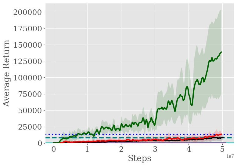
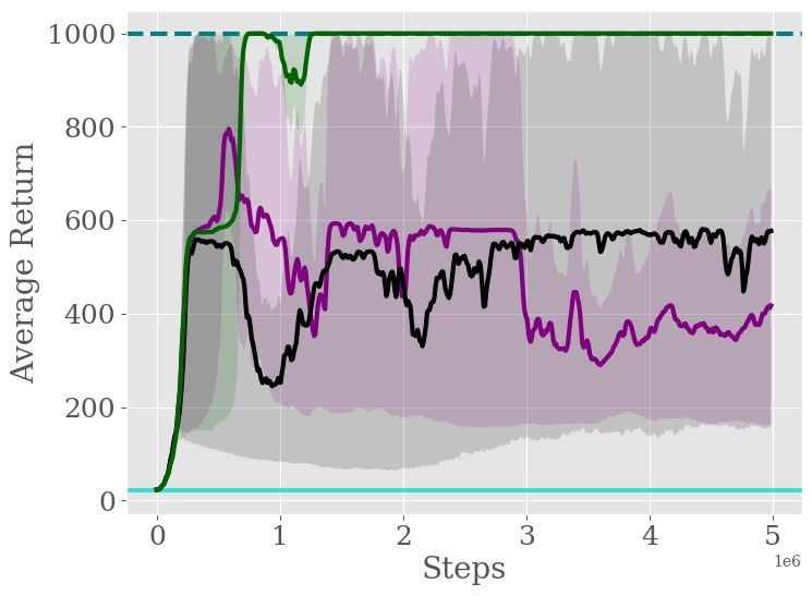
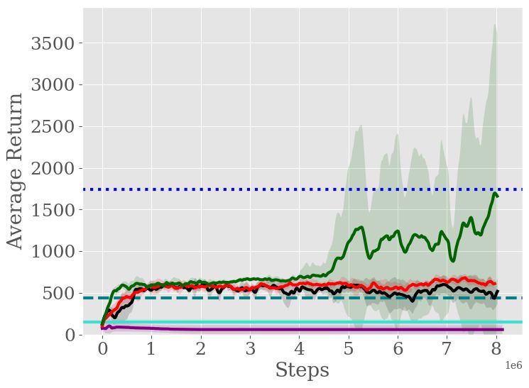
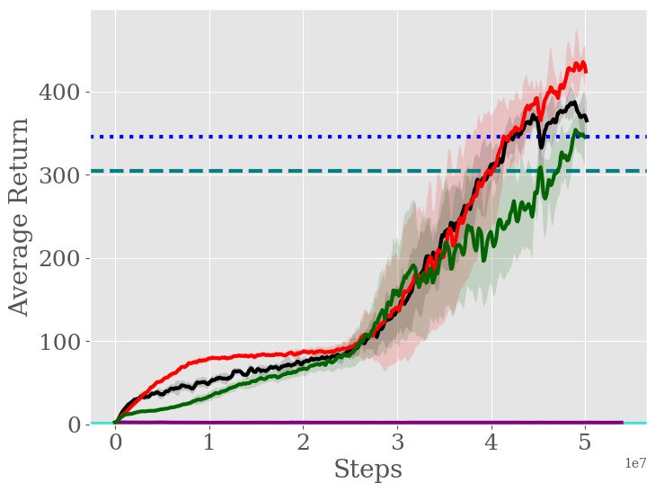
Under review as a conference paper at ICLR 2021

 (a) Kung-Fu Master. (b) Battle Zone. (c) Centipede. (d) Seaquest.

 (e) Q*bert. (f) Breakout. (g) Beam Rider. (h) Space Invaders.

Figure 4: Average return vs. the number of simulation steps on Atari games. The solid lines show
the mean performance over five random seeds. The shaded area represents the standard deviation
from the mean. The blue dotted line denotes the average return of the expert. The area above the blue
dotted line indicates performance beyond the expert.

4.1.1 H OW DOES V PERL OUTPERFORM PREVIOUS METHODS ?

The contributions of each component of vPERL. In this subsection, we study the contribution of
each component of our method, i.e. Action Back-tracing submodule, Transition Modeling submodule,
and the variational objective in Eq. (1). Specifically, we directly train the Action Back-tracing and
Transition Modeling submodules in terms of supervised learning. We used the mean of the reward
map and the prediction error of the next state as the reward for the former and latter submodules,
respectively. To study the contribution of the variational objective, we introduced another baseline,
PERL, which trains both submodules as an autoencoder. Table 3 shows quantitative comparison
between the performance of vPERL and its components.

Table 3: Average return of vPERL-Small-RMean , and its components (i.e., Action Back-tracing and
Transition Modeling, and PERL) with one-life demonstration data on eight Atari games. The results
shown are the mean performance over five random seeds with better-than-expert performance in bold.
 Expert Demo. vPERL-Small-RMean Components of vPERL-Small-RMean
 Game Average Average Average Action Back-tracing Transition Modeling PERL Supervised PERL
 Kung-Fu Master 23,434.8 6,500.0 20,518.3 0.0 0.0 0.0 0.0
 Battle Zone 18,137.5 7,000.0 21,899.1 6000.0 0.0 0.0 2,000.0
 Centipede 4,069.4 360.0 21,113.4 151.0 2,216.7 16,479.6 2,485.1
 Seaquest 1,744.5 440.0 1,634.2 0.0 0.0 140.0 80.0
 Q*bert 13,441.5 8,150.0 135,598.0 74.9 150.0 0.0 0.0
 Breakout 346.4 305.0 348.8 2.5 5.5 2.2 2.7
 Beam Rider 2,447.7 1,332.0 3,801.8 22.0 784.8 17.6 0.0
 Space Invaders 734.1 600.0 1,106.5 285.0 145.5 285.0 0.0

The results show that individual training of each component results in no avail. PERL successfully
outperforms the demonstration in one game, i.e. Centipede, which indicates the potential advantage
of using both submodules. However, PERL fails in the other seven games, while vPERL outperforms
the demonstration in eight games and outperforms expert in six. The large performance gap between
PERL and vPERL indicates the variational objective in Eq. (1) is important to learn efficient rewards.
To further investigate the key reason for why our method works well, we added another baseline -
supervised PERL, which forces the encoding of PERL to be close to the true action. The supervised
PERL fails in all of the games. Comparing with vPERL, we can attribute the critical contribution to
the use of the ELBO of conditional VAE, or more specific, the term KL(qφ (z|st , st+1 )kpθ (z|st )) in
Eq. (1). It helps vPERL to work well and outperform previous methods for two reasons:
1) The generative training of VAE can serve as a good regularization to alleviate the overfitting
problem.

 7

Under review as a conference paper at ICLR 2021

2) The regularization enables vPERL to learn a smooth value function and reward function, which
consistently provides straightforward and informative rewards for the moving states in the environ-
ment.
Empirical evidence:
1) Better generalization ability. The empirical results in Table 2 and Figure 4 show that VIN, GAIL
and VAIL are vulnerable to overfitting problem, usually results in no avail and has fewer chances to
reach the demonstration-level performance. In contrast, our vPERL has better generalization ability
and consistently achieves performance that is either close to or better than the expert.
2) Straightforward and informative reward. Figure 5 shows the state, the reward maps of vPERL
and GIRIL in three Atari games. The reward map of GIRIL can be close to zero (in Battle Zone) and
state (in Q*bert) or occasionally informative (in Centipede), which is ambiguous and less informative.
In contrast, the reward map of our vPERL is more straightforward, and consistently attends to
informative regions in the state for all of the games.

 State vPERL reward GIRIL reward State vPERL reward GIRIL reward State vPERL reward GIRIL reward

 (a) Battle Zone (b) Centipede (c) Q*bert

 Figure 5: Visualization of state, vPERL reward map and GIRIL reward map for Atari games.

Our method successfully addresses the two key issues, therefore, it can outperform previous methods.

4.2 C ONTINUOUS C ONTROL TASKS

We also evaluated our method on continuous control tasks where the state space is low-dimensional
and the action space is continuous. The continuous control tasks were from Pybullet 1 environment.
Demonstrations To generate demonstrations, we trained a Proximal Policy Optimization (PPO)
agent with the ground-truth reward for 1 million simulation steps. We used the PPO implementation
in the repository (Kostrikov, 2018) with the default hyper-parameters for continuous control tasks.
In each task, we used one demonstration with a fixed length of 1,000 for evaluation. The details of
experimental setup can be found in Appendix F.1.
Results Figure 6 shows that our method
vPERL achieves the best imitation perfor-
mance in both continuous control tasks, i.e.
Inverted Pendulum and Inverted Double
Pendulum. Although GIRIL achieves per-
formance that is close to the demonstration,
the efficient planning-based reward func-
tion enables vPERL to perform even bet-
ter. Other baselines are unable to reach the
demonstration-level performance by learn- (a) Inverted Pendulum. (b) Inverted Double Pendulum.
ing from only one demonstration. Quanti- Figure 6: Average return vs. number of simulation steps
tative results are shown in Appendix A. on continuous control tasks.

4.3 A BLATION S TUDIES

Ablation study on the growing number of demonstrations. Figure 7 shows the average return
versus number of full-episode demonstrations on both Atari games and continuous control tasks. The
results shows that our method vPERL achieves the highest performance across different numbers
of full-episode demonstrations. GIRIL usually comes the second best, and GAIL can achieve good
performance with more demonstrations in continuous control tasks. Quantitative results have been
shown in Appendix B.1.
 1
 https://pybullet.org/

 8

Under review as a conference paper at ICLR 2021

 (a) Centipede. (b) Qbert. (c) Inverted Pendulum. (d) Inverted Double Pendulum.

Figure 7: Average return vs. number of demonstrations on Atari games and continuous control tasks.

Ablation study on the optimality of the demonstrations. Figure 8 shows the average return versus
optimality of demonstrations on Atari games and continuous control tasks. In sections 4.1 and 4.2, we
trained PPO agents with ground-truth reward for 10 million (10M) steps as the expert for Atari games,
and for 1 million (1M) steps as the expert for continuous control tasks. In this ablation, we train PPO
agents with 10% and 50% simulation steps of the expert to generate demonstrations with diverse
optimality. The results show that vPERL consistently outperforms the expert and demonstrations on
the demonstrations of different optimality. Quantitative results are shown in Appendix B.2.

 (a) Centipede. (b) Qbert. (c) Inverted Pendulum. (d) Inverted Double Pendulum.

Figure 8: Average return vs. number of the expert simulation steps (NE ) on Atari games and
continuous control tasks.

Ablation study on the hyper-parameters K. Figure 8 shows the average return versus different
choices of K on Atari games and continuous control tasks. The results show that our method is not
very sensitive to different choices of K. Quantitative results are shown in Appendix B.3.

 (a) Centipede. (b) Qbert. (c) Inverted Pendulum. (d) Inverted Double Pendulum.

 Figure 9: Average return vs. choices of K on Atari games and continuous control tasks.

5 C ONCLUSION
This paper presents a simple but efficient reward learning method, called variational planning-
embedded reward learning (vPERL). By simultaneously training a planning-embedded action back-
tracing module and a transition dynamics module in a unified generative solution, we obtain a
reward function that is straightforward and informative, and has better generalization ability than
previous methods. Informative analysis and empirical evidence support the critical contribution
of ELBO regularization term for learning efficient planning-based reward with extremely limited
demonstrations. Empirical results show our method outperforms state-of-the-art imitation learning
methods on multiple Atari games and continuous control tasks by a large margin. Extensive ablation
studies show that our method is not very sensitive to the number of demonstrations, optimality of
demonstration, and choices of the hyperparameter K. We remain the extension of our method to more
complex continuous control tasks as future work. Another interesting topic for future investigation
would be applying vPERL to hard exploration tasks with extremely sparse rewards.

 9

Under review as a conference paper at ICLR 2021

R EFERENCES
Pieter Abbeel and Andrew Y Ng. Apprenticeship learning via inverse reinforcement learning. In
 International Conference on Machine Learning, pp. 1, 2004.
Richard Bellman. A markovian decision process. Journal of mathematics and mechanics, pp.
 679–684, 1957.
Richard Bellman. Dynamic programming. Science, 153(3731):34–37, 1966.
Abdeslam Boularias, Jens Kober, and Jan Peters. Relative entropy inverse reinforcement learning. In
 International Conference on Artificial Intelligence and Statistics, pp. 182–189, 2011.
Greg Brockman, Vicki Cheung, Ludwig Pettersson, Jonas Schneider, John Schulman, Jie Tang, and
 Wojciech Zaremba. Openai gym. arXiv preprint arXiv:1606.01540, 2016.
Daniel S Brown, Wonjoon Goo, Prabhat Nagarajan, and Scott Niekum. Extrapolating beyond
 suboptimal demonstrations via inverse reinforcement learning from observations. In International
 Conference on Machine Learning, 2019a.
Daniel S Brown, Wonjoon Goo, and Scott Niekum. Ranking-based reward extrapolation without
 rankings. In Conference on Robot Learning, 2019b.
Chelsea Finn, Sergey Levine, and Pieter Abbeel. Guided cost learning: Deep inverse optimal control
 via policy optimization. In International Conference on Machine Learning, pp. 49–58, 2016.
Ian Goodfellow, Jean Pouget-Abadie, Mehdi Mirza, Bing Xu, David Warde-Farley, Sherjil Ozair,
 Aaron Courville, and Yoshua Bengio. Generative adversarial nets. In Advances in Neural
 Information Processing Systems, pp. 2672–2680, 2014.
Jonathan Ho and Stefano Ermon. Generative adversarial imitation learning. In Advances in Neural
 Information Processing Systems, pp. 4565–4573, 2016.
Borja Ibarz, Jan Leike, Tobias Pohlen, Geoffrey Irving, Shane Legg, and Dario Amodei. Reward
 learning from human preferences and demonstrations in atari. In Advances in Neural Information
 Processing Systems, pp. 8011–8023, 2018.
Animesh Karnewar. Pytorch implementations of variational discriminator bottleneck, 2018. URL
 https://github.com/akanimax/Variational_Discriminator_Bottleneck.
Diederik P Kingma and Jimmy Ba. Adam: A method for stochastic optimization. In International
 Conference on Learning Representations, 2015.
Diederik P Kingma and Max Welling. Auto-encoding variational bayes. arXiv preprint
 arXiv:1312.6114, 2013.
Ilya Kostrikov. Pytorch implementations of reinforcement learning algorithms, 2018. URL https:
 //github.com/ikostrikov/pytorch-a2c-ppo-acktr-gail.
Nantas Nardelli, Gabriel Synnaeve, Zeming Lin, Pushmeet Kohli, Philip HS Torr, and Nicolas
 Usunier. Value propagation networks. In International Conference on Learning Representations,
 2019.
Andrew Y Ng and Stuart J Russell. Algorithms for inverse reinforcement learning. In International
 Conference on Machine Learning, volume 1, pp. 663–670, 2000.
Sufeng Niu, Siheng Chen, Hanyu Guo, Colin Targonski, Melissa C Smith, and Jelena Kovačević.
 Generalized value iteration networks: Life beyond lattices. In AAAI Conference on Artificial
 Intelligence, 2018.
Xue Bin Peng, Angjoo Kanazawa, Sam Toyer, Pieter Abbeel, and Sergey Levine. Variational
 discriminator bottleneck: Improving imitation learning, inverse rl, and gans by constraining
 information flow. In International Conference on Learning Representations, 2019.

 10

Under review as a conference paper at ICLR 2021

Dean A Pomerleau. Efficient training of artificial neural networks for autonomous navigation. Neural
 Computation, 3(1):88–97, 1991.
Martin L Puterman. Markov Decision Processes: Discrete Stochastic Dynamic Programming. John
 Wiley & Sons, 2014.
John Schulman, Philipp Moritz, Sergey Levine, Michael Jordan, and Pieter Abbeel. High-dimensional
 continuous control using generalized advantage estimation. In International Conference on
 Learning Representations, 2016.
John Schulman, Filip Wolski, Prafulla Dhariwal, Alec Radford, and Oleg Klimov. Proximal policy
 optimization algorithms. arXiv preprint arXiv:1707.06347, 2017.
Kihyuk Sohn, Honglak Lee, and Xinchen Yan. Learning structured output representation using
 deep conditional generative models. In Advances in neural information processing systems, pp.
 3483–3491, 2015.
Aviv Tamar, Yi Wu, Garrett Thomas, Sergey Levine, and Pieter Abbeel. Value iteration networks. In
 Advances in Neural Information Processing Systems, pp. 2154–2162, 2016.
Xingrui Yu, Yueming Lyu, and Ivor Tsang. Intrinsic reward driven imitation learning via generative
 model. In International Conference on Machine Learning, pp. 6672–6682, 2020.
Li Zhang, Xin Li, Sen Chen, Hongyu Zang, Jie Huang, and Mingzhong Wang. Universal value
 iteration networks: When spatially-invariant is not universal. In AAAI Conference on Artificial
 Intelligence, pp. 2154–2162, 2020.
Brian D Ziebart, Andrew Maas, J Andrew Bagnell, and Anind K Dey. Maximum entropy inverse
 reinforcement learning. In AAAI Conference on Artificial Intelligence, 2008.
Brian D Ziebart, J Andrew Bagnell, and Anind K Dey. Modeling interaction via the principle of
 maximum causal entropy. In International Conference on Machine Learning, 2010.

 11

Under review as a conference paper at ICLR 2021

A Q UANTITATIVE RESULTS OF CONTINUOUS CONTROL TASKS .

Table 4 shows the detailed quantitative comparison of the demonstration and imitation methods. The
results shown in the table were the mean performance over three random seeds.

Table 4: Average return of vPERL, GIRIL, VIN and state-of-the-arts inverse reinforcement learning
algorithms GAIL (Ho & Ermon, 2016) and VAIL (Peng et al., 2019) with one demonstration data on
continuous control tasks. The results shown are the mean performance over 3 random seeds with best
imitation performance in bold.
 Demonstration vPERL Imitation Learning Algorithms
 Task Average RMean GIRIL VAIL GAIL VIN
 Inverted Pendulum 1,000.0 1,000.0 993.2 520.1 572.2 21.0
 Inverted Double Pendulum 9,355.1 9,357.8 9,184.5 539.8 519.6 181.1

B A BLATION STUDIES

B.1 T HE EFFECT OF THE NUMBER OF FULL - EPISODE DEMONSTRATIONS .

We also evaluated our method with different numbers of full-episode demonstrations on both Atari
games and continuous control tasks. Table 5 and Table 6 show the detailed quantitative comparison of
imitation learning methods across different numbers of full-episode demonstrations in the Centipede
game and Qbert game. The comparisons on two continuous control tasks, Inverted Pendulum and
Inverted Double Pendulum, have been shown in Table 7 and Table 8.
The results shows that our method vPERL achieves the highest performance across different numbers
of full-episode demonstrations, and GIRIL usually comes the second best. GAIL is able to achieve
better performance with the increase of the demonstration number in both continuous control tasks.

Table 5: Parameter Analysis of the vPERL versus other baselines with different numbers of full-
episode demonstrations on Centipede game. The results shown are the mean performance over 5
random seeds with best performance in bold.
 # Demonstrations vPERL GIRIL VAIL GAIL
 1 13,253.2 9,195.1 4,212.8 171.0
 5 21,219.2 2,952.5 2,465.6 161.0
 10 14,406.2 8,599.6 3,108.0 2,232.4

Table 6: Parameter Analysis of the vPERL versus other baselines with different numbers of full-
episode demonstrations on Qbert game. The results shown are the mean performance over 5 random
seeds with best performance in bold.
 # Demonstrations vPERL GIRIL VAIL GAIL
 1 200,455.0 11,105.0 13,695.0 0.0
 5 200,450.0 13,740.0 13,300.0 0.0
 10 192,962.5 12,327.5 10,852.5 0.0

Table 7: Parameter Analysis of the vPERL versus other baselines with different numbers of full-
episode demonstrations on Inverted Pendulum task. The results shown are the mean performance
over 5 random seeds with best performance in bold.
 # Demonstrations vPERL GIRIL VAIL GAIL
 1 1,000.0 993.2 520.1 572.2
 5 1,000.0 1,000.0 68.2 591.2
 10 1,000.0 1,000.0 41.8 1,000.0

 12

Under review as a conference paper at ICLR 2021

Table 8: Parameter Analysis of the vPERL versus other baselines with different numbers of full-
episode demonstrations on InvertedDoublePendulum task. The results shown are the mean perfor-
mance over 5 random seeds with best performance in bold.
 # Demonstrations vPERL GIRIL VAIL GAIL
 1 9,357.8 9,184.5 539.8 519.6
 5 9,352.4 9,317.2 372.5 9,342.5
 10 9,353.1 9,314.1 274.6 9,352.1

B.2 T HE EFFECT OF EXPERT OPTIMALITY.

Table 9 and Table 10 show the average return of vPERL-Small-RMean with demonstrations of
different optimality on Atari games and continuous control tasks, respectively. In the experiments, we
trained a PPO agent with ground-truth reward for 10 million (10M) simulation steps as the expert for
Atari games, and 1 million (1M) steps for continuous control tasks. To study the effects of optimality
of the demonstrations, we additionally trained PPO agents with less simulation steps: 1M steps and
5M steps for Atari games, and 0.1M steps and 0.5M steps for continuous control tasks. With the
additional PPO agents, we generated demonstrations with 10%, 50% optimality of the 10M-step
‘Expert’ for both Atari games and continuous control tasks.
The results show that our method outperforms expert by a large margin in Atari games and reach
the demonstration-level performance in continuous control tasks with demonstrations of different
optimality.

Table 9: Average return of vPERL-Small-RMean with one-life demonstration data of expert policy
trained under different simulations steps (NE =1 million, 5 million and 10 million). The results shown
are the mean performance over five random seeds with better-than-expert performance in bold.
 Expert Demonstration vPERL-Small-RMean
 Game Average Average NE =1M NE =5M NE =10M
 Battle Zone 18,137.5 7,000.0 24,800.0 34,897.2 21,899.1
 Centipede 4,069.4 360.0 16,343.7 17,223.3 21,113.4
 Q*bert 13,441.5 8,150.0 147,565.5 200,300.0 135,598.0
 Beam Rider 2,447.7 1,332.0 3,374.4 3,256.0 3,801.8

Table 10: Average return of vPERL-RMean with one demonstration data of expert policy trained
under different simulations steps (NE =0.1 million, 0.5 million and 1 million). The results shown are
the mean performance over five random seeds with demonstration-level performance in bold.
 Demonstration vPERL-RMean
 Game Average NE =0.1M NE =0.5M NE =1M
 Inverted Pendulum 1,000 1,000.0 1,000.0 1,000.0
 Inverted Double Pendulum 9,355.1 9,351.9 9,350.8 9,357.8

B.3 T HE EFFECT OF CHOICES OF K.

For the sake of consistency, we set K = 10 for all of experiments on Atari games and continuous
control tasks in Section 4. To study the effects of the hyperparameter K, we evaluate our method on
two Atari games and two continuous control tasks with two additional K (K=5, and K=15).
Table 11 and Table 12 shows the average return of vPERL-Small-RMean versus different choices of
K on Atari games and continuous control tasks. With the three choices of K, our method consistently
outperforms the expert in the Atari games, and reach the best (demonstration-level) performance
in continuous control tasks. This indicates that our method is not very sensitive to the choices of
hyperparameter K.

 13

Under review as a conference paper at ICLR 2021

Table 11: Average return of vPERL-Small-RMean with different choices of K, on one-life demonstra-
tion data. The results shown are the mean performance over five random seeds with better-than-expert
performance in bold.
 Expert Demo. vPERL-Small-RMean
 Game Average Average K=5 K=10 K=15
 Centipede 4,069.4 360.0 19,228.8 21,113.4 18,776.2
 Q*bert 13,441.5 8,150.0 46,705.5 135,598.0 173,735.0

Table 12: Average return of vPERL-RMean with different choices of K, on one-life demonstration
data. The results shown are the mean performance over five random seeds with demonstration-level
performance in bold.
 Demonstration vPERL-RMean
 Game Average K=5 K=10 K=15
 Inverted Pendulum 1,000 1,000.0 1,000.0 1,000.0
 Inverted Double Pendulum 9,355.1 9,358.8 9,357.8 9,351.9

C A DDITIONAL EVALUATION RESULTS

C.1 A DDITIONAL ATARI GAMES .

Table 13 shows the average return of vPERL-Small with RMean and other baselines on two additional
Atari games, Krull and Time Pilot. The results show that our method outperforms the expert and
other baselines by a large margin on both additional Atari games.

Table 13: Average return of vPERL-Small with RMean , GIRIL (Yu et al., 2020), VIN and state-
of-the-art IRL algorithms GAIL (Ho & Ermon, 2016) and VAIL (Peng et al., 2019) with one-life
demonstration data on additional Atari games. The results shown are the mean performance over five
random seeds with better-than-expert performance in bold.
 Expert Demo. vPERL-Small Imitation Learning Algorithms
 Game Average Average RMean GIRIL VAIL GAIL VIN
 Krull 8,262.0 2,826.0 19,412.5 6,515.0 5,819.7 264.0 2,013.3
 Time Pilot 4,200.0 100.0 4,400.0 3,680.0 2,080.0 400.0 2,572.0

C.2 O NE - LIFE DEMONSTRATIONS WITHOUT SCORES AND LIVES ON THE STATES .

To avoid the effects of the scores and lives in the states of Atari games, we also evaluate our method
on the “No-score Demo.”, which is obtained by masking the game score and number of lives left in the
demonstrations (Brown et al., 2019a). Table 14 compares the average return of vPERL-Small-RMean
with the “Standard Demo.” and the “No-score Demo.” on Q*bert game and Krull game.

Table 14: Average return of vPERL-Small-RMean with different choices of K on one-life demonstra-
tion data. The results shown are the mean performance over five random seeds with better-than-expert
performance in bold.
 Expert Demo. vPERL-Small-RMean
 Game Average Average Standard Demo. No-score Demo.
 Krull 8,262.0 2,826.0 19,412.5 27,009.6
 Q*bert 13,441.5 8,150.0 135,598.0 200,500.0

The results show that our method achieves better performance on the “No-score Demo.” than the
“Standard Demo.”. This indicates the negative effects of the game scores and numbers of left lives
on the states of demonstrations. From Figure 1 and more reward visualization in Section D and
E, we observe that our method learns to attend on the meaningful region in a state and ignore the
game score and numbers of left lives automatically. Masking the game score and numbers of left

 14

Under review as a conference paper at ICLR 2021

lives in the demonstration further alleviates burdens on learning efficient planning computations and
planning-based rewards for Atari games.
In summary, our method can learn to outperform the expert without explicitly access to the true
rewards, and does not relied on the game scores and numbers of left lives in the states of demonstra-
tions. Furthermore, the results show that the performance of our method can be improved by masking
out the game scores and numbers of left lives in the demonstrations.

D V ISUALIZATION OF REWARD AND VALUE IMAGES OF VPERL-L ARGE AND
 VIN.
In this section, we visualize the reward maps and value maps learned by vPERL-Large and VIN
on Atari games. Here, both vPERL and VIN are based on large-size VIN architecture. The size of
reward map is 84 × 84. The figures show that the reward and value maps learned by vPERL are much
meaningful than that by VIN.

 (a) State. (b) vPERL Reward and Value. (c) VIN Reward and Value.

Figure 10: Visualization of state, reward map and value map on Battle Zone game. (a) The state, (b)
the reward map and value map of vPERL, and (c) the reward map and value map of VIN.

 (a) State. (b) vPERL Reward and Value. (c) VIN Reward and Value.

Figure 11: Visualization of state, reward map and value map on Centipede game. (a) The state, (b)
the reward map and value map of vPERL, and (c) the reward map and value map of VIN.

 (a) State. (b) vPERL Reward and Value. (c) VIN Reward and Value.

Figure 12: Visualization of state, reward map and value map on Seaquest game. (a) The state, (b) the
reward map and value map of vPERL, and (c) the reward map and value map of VIN.

 15

Under review as a conference paper at ICLR 2021

 (a) State. (b) vPERL Reward and Value. (c) VIN Reward and Value.

Figure 13: Visualization of state, reward map and value map on Qbert game. (a) The state, (b) the
reward map and value map of vPERL, and (c) the reward map and value map of VIN.

 (a) State. (b) vPERL Reward and Value. (c) VIN Reward and Value.

Figure 14: Visualization of state, reward map and value map on Breakout game. (a) The state, (b) the
reward map and value map of vPERL, and (c) the reward map and value map of VIN.

 (a) State. (b) vPERL Reward and Value. (c) VIN Reward and Value.

Figure 15: Visualization of state, reward map and value map on Space Invaders game. (a) The state,
(b) the reward map and value map of vPERL, and (c) the reward map and value map of VIN.

 16

Under review as a conference paper at ICLR 2021

E V ISUALIZATION OF REWARD AND VALUE IMAGES OF VPERL-S MALL AND
 VIN.
In this section, we visualize the reward maps and value maps learned by vPERL and VIN on several
Atari games. To enable faster training, here both vPERL and VIN are based on small-size VIN
architecture. The size of reward map is 18 × 18. The figures show that the reward and value maps
learned by vPERL are much meaningful than that by VIN.

 (a) State. (b) vPERL Reward and Value. (c) VIN Reward and Value.

Figure 16: Visualization of state, reward map and value map on Kung-Fu Master game. (a) The state,
(b) the reward map and value map of vPERL, and (c) the reward map and value map of VIN.

 (a) State. (b) vPERL Reward and Value. (c) VIN Reward and Value.

Figure 17: Visualization of state, reward map and value map on Battle Zone game. (a) The state, (b)
the reward map and value map of vPERL, and (c) the reward map and value map of VIN.

 (a) State. (b) vPERL Reward and Value. (c) VIN Reward and Value.

Figure 18: Visualization of state, reward map and value map on Centipede game. (a) The state, (b)
the reward map and value map of vPERL, and (c) the reward map and value map of VIN.

 (a) State. (b) vPERL Reward and Value. (c) VIN Reward and Value.

Figure 19: Visualization of state, reward map and value map on Seaquest game. (a) The state, (b) the
reward map and value map of vPERL, and (c) the reward map and value map of VIN.

 17

Under review as a conference paper at ICLR 2021

 (a) State. (b) vPERL Reward and Value. (c) VIN Reward and Value.

Figure 20: Visualization of state, reward map and value map on Qbert game. (a) The state, (b) the
reward map and value map of vPERL, and (c) the reward map and value map of VIN.

 (a) State. (b) vPERL Reward and Value. (c) VIN Reward and Value.

Figure 21: Visualization of state, reward map and value map on Breakout game. (a) The state, (b) the
reward map and value map of vPERL, and (c) the reward map and value map of VIN.

 (a) State. (b) vPERL Reward and Value. (c) VIN Reward and Value.

Figure 22: Visualization of state, reward map and value map on Space Invaders game. (a) The state,
(b) the reward map and value map of vPERL, and (c) the reward map and value map of VIN.

 (a) State. (b) vPERL Reward and Value. (c) VIN Reward and Value.

Figure 23: Visualization of state, reward map and value map on Beam Rider game. (a) The state, (b)
the reward map and value map of vPERL, and (c) the reward map and value map of VIN.

F A DDITIONAL D ETAILS OF E XPERIMENTAL S ETUPS

F.1 E XPERIMENTAL SETUP OF CONTINUOUS CONTROL TASKS

Our first step was also to train a reward learning module for each continuous control task on one
demonstration. To build our reward learning module for continuous tasks, we used a simple VIN
and inverse VIN as the model bases of action back-tracing and transition modeling submodules,
respectively. In the simple VIN model, we used 1D convolutional layer with a kernel size of 2 and

 18

Under review as a conference paper at ICLR 2021

stride of 1 to implement the function fR , reward map R and Q value Q. To accomplish the action
back-tracing, the final value map of VIN was fully connected with a hidden layer with a size of 32.
Reversely, we used 1D deconvolutional layer to implement the inverse VIN model. We kept the size
of feature maps in both VIN and inverse VIN unchanged across all the layers. We set K = 10 for both
the VIN and inverse VIN in all tasks. The dimension of latent variable z is set to the action dimension
for each task. Additionally, we used a two-layer feed forward neural network with tanh activation
function as policy architecture. The number of hidden unit is set to 100 for all tasks. To extend our
method on continuous control tasks, we made minor modification on the training objective. In Atari
games, we used the KL divergence to measure the distance between the expert policy distribution and
the action distribution in Eq. (1). In continuous control tasks, we instead directly treated the latent
variable z as the back-traced action and used mean squared error to measure the distance between
the back-traced action and the true action in the demonstration. We set the scaling weight α in Eq.
(1) to 1.0 for all tasks. Training was conducted with the Adam optimizer (Kingma & Ba, 2015) at
a learning rate of 3e-5 and a mini-batch size of 32 for 50, 000 epochs. In each training epoch, we
sampled a mini-batch of data every 20 states.
To evaluate the quality of our learned reward, we used the trained reward learning module to produce
rewards, and trained a policy to maximize the inferred reward function via PPO. We trained the PPO
on the learned reward function for 5 million simulation steps to obtain our final policy. The PPO is
trained with a learning rate of 3e-4, a clipping threshold of 0.1, a entropy coefficient of 0.0, a value
function coefficient of 0.5, and a GAE parameter of 0.95 (Schulman et al., 2016).
For a fair comparison, we used the same VIN as the model base for all the baselines. The reward
function of GAIL and VAIL was chosen according to the original papers (Ho & Ermon, 2016; Peng
et al., 2019). The information constraint Ic in VAIL was set to 0.5 for all tasks. To enable fast training,
we trained all the imitation methods with 16 parallel processes.

F.2 A DDITIONAL DETAILS OF GAIL AND VAIL

The discriminator for both GAIL and VAIL takes in a state (a stack of four frames) and an action
(represented as a 2d one-hot vector with a shape of (|A| × 84 × 84), where |A| is the number of
valid discrete actions in each environment) (Brown et al., 2019b). The discriminator outputs a
binary classification value, and − log(D(s, a)) is the reward. VAIL was implemented according
to the repository of Karnewar (2018). The discriminator network architecture has an additional
convolutional layer (with a kernel size of 4) as the final convolutional layer to encode the latent
variable in VAIL. We used the default setting of 0.2 for the information constraint (Karnewar, 2018).
PPO with the same hyper-parameters was used to optimize the policy network for all the methods.
For both GAIL and VAIL, we trained the discriminator using the Adam optimizer with a learning
rate of 0.001. The discriminator was updated at each policy step.

 19