Travelers' Bi-Attribute Decision Making on the Risky Mode Choice with Flow-Dependent Salience Theory - MDPI
←
→
Page content transcription
If your browser does not render page correctly, please read the page content below
sustainability

Article
Travelers’ Bi-Attribute Decision Making on the Risky Mode
Choice with Flow-Dependent Salience Theory
Xiangfeng Ji *            and Xiaoyu Ao

                                          Department of Management Science and Engineering, School of Business, Qingdao University,
                                          Qingdao 266071, China; aoxiaoyu@qdu.edu.cn
                                          * Correspondence: jixiangfeng@qdu.edu.cn

                                          Abstract: The purpose of this paper is to provide new insights into travelers’ bi-attribute (travel
                                          time and travel cost) risky mode choice behavior with one risky option (i.e., the highway) and
                                          one non-risky option (i.e., the transit) from the long-term planning perspective. In the classical
                                          Wardropian User Equilibrium principle, travelers make their choice decisions only based on the
                                          mean travel times, which might be an unrealistic behavioral assumption. In this paper, an alternative
                                          approach is proposed to partially remedy this unrealistic behavioral assumption with flow-dependent
                                          salience theory, based on which we study travelers’ context-dependent bi-attribute mode choice
                                          behavior, focusing on the effect of travelers’ salience characteristic. Travelers’ attention is drawn
                                          to the bi-attribute salient travel utility, and then the objective probability of each state for the risky
                                          world is distorted in favor of this bi-attribute salient travel utility. A long-term bi-attribute salient
                                          user equilibrium will be achieved when no traveler can improve their bi-attribute salient travel utility
                                          by unilaterally changing the choice decisions. Conditions for the existence and uniqueness of the
                                          bi-attribute salient user equilibrium are presented, and based on the equilibrium results, we analyze
                                travelers’ risk attitudes in this bi-attribute risky choice problem. Finally, numerical examples are

                                          conducted to examine the sensitivity of equilibrium solutions to the input parameters, which are cost
Citation: Ji, X.; Ao, X. Travelers’
                                          difference and salience bias.
Bi-Attribute Decision Making on the
Risky Mode Choice with
                                          Keywords: bi-attribute choice behavior; salient travel utility; salient user equilibrium; cost difference;
Flow-Dependent Salience Theory.
                                          behavioral insights
Sustainability 2021, 13, 3901.
https://doi.org/10.3390/su13073901

Academic Editor: Luca D’Acierno
                                          1. Introduction
Received: 28 February 2021                      One of the powerful principles widely used in the traditional four-step transportation
Accepted: 20 March 2021                   planning model is the Wardrop’s user equilibrium model, also known as Wardrop’s first
Published: 1 April 2021                   principle proposed in [1], which can be stated as: No traveler can decrease his (her) travel
                                          time by unilaterally changing his (her) choice decisions. In this paper, we use this principle
Publisher’s Note: MDPI stays neutral      to study travelers’ mode choice behavior as [2].
with regard to jurisdictional claims in         There are several unrealistic assumptions underlying this principle. One of these
published maps and institutional affil-
                                          is that travel times on the traffic network are deterministic. However, several studies
iations.
                                          show that uncertainty is inevitable, which could come from the demand side, and/or the
                                          supply side (e.g., [3,4]). Numerous studies that consider the uncertainty on the traffic
                                          network have been conducted. For example, the authors in [5] classified the travelers into
                                          three categories on the stochastic traffic network, which are risk-neutral, risk-seeking and
Copyright: © 2021 by the authors.         risk-averse. The authors in [6] incorporated the random evolution of traffic states in the
Licensee MDPI, Basel, Switzerland.        cell-based multi-class dynamic traffic assignment. The authors in [7] studied a risk-neutral
This article is an open access article    congestion pricing problem and formulated it as a stochastic programming problem. The
distributed under the terms and
                                          authors in [8] proposed a general approach to incorporate stochastic variations into the
conditions of the Creative Commons
                                          macroscopic traffic model. The authors in [9] studied a simultaneous route and departure
Attribution (CC BY) license (https://
                                          time choice problem with stochastic travel times, where the demand is fixed and the link
creativecommons.org/licenses/by/
                                          capacity is stochastic. The work of [10] classified uncertainty during the decision making
4.0/).

Sustainability 2021, 13, 3901. https://doi.org/10.3390/su13073901                                    https://www.mdpi.com/journal/sustainability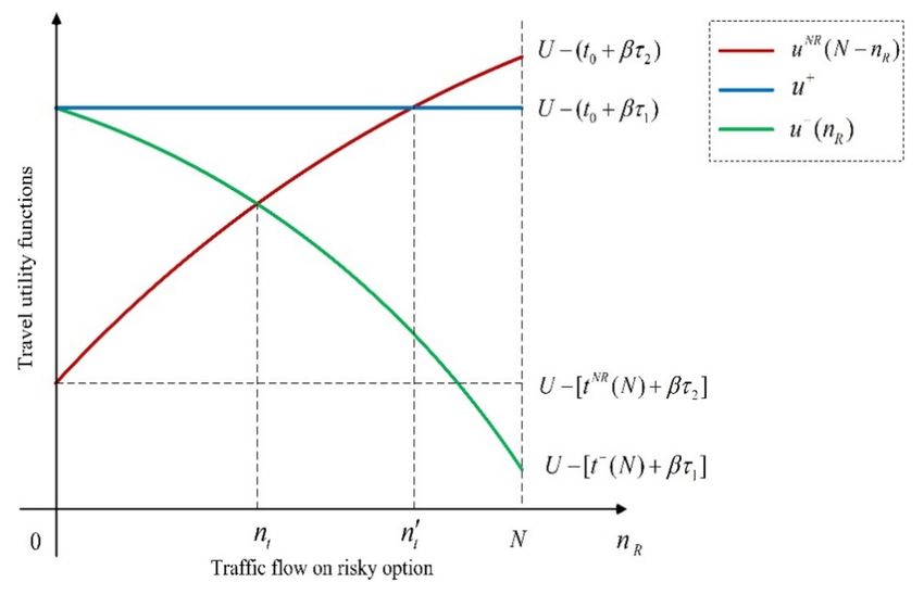
Sustainability 2021, 13, 3901                                                                                                2 of 24

                                into two kinds, risk and ambiguity. The difference between risk and ambiguity is whether
                                the probability distribution of the uncertainty is known or not. For the risk analysis, it is
                                known, while it is not known for the ambiguity analysis. Our study in this paper belongs
                                to the decision making analysis under risk.
                                      Another assumption underlying the user equilibrium principle is that only travel time
                                is considered in travelers’ choice decision. However, it has been empirically demonstrated
                                that traveler’s choice behavior might be affected by several different attributes, e.g., travel
                                time, travel time reliability, travel cost, schedule delay, travel distance, and so on (e.g., [11]).
                                The authors in [11] showed that the three most important factors influencing traveler’s
                                choice behavior are shorter travel time, travel time reliability and shorter distance. From
                                the statistical analysis, 40% of the total respondents select shorter travel time as the first
                                reason, 32% of these respondents select travel time reliability as the second reason, and
                                31% of these respondents select shorter distance as the third reason. Note here that the sum
                                is bigger than 100%, because some respondents indicate more than one attributes as the
                                most important. Scholars have also made substantial progress in travelers’ multi-attribute
                                analysis theoretically. For example, the authors in [12] combined the travel time and travel
                                cost as the generalized cost. The authors in [13] discussed the weighted sum of travel
                                time and travel time reliability and proposed the travel time budget (TTB) model. The
                                authors in [3] proposed the mean-excess travel time (METT) model based on the TTB model,
                                where travel time, travel time reliability and travel time unreliability are incorporated. The
                                authors in [14] incorporated the day-to-day variations into the TTB model, and proposed a
                                subjective-utility TTB model. The authors in [15] presented the non-expected route travel
                                time model, which generalized TTB model and METT model. The authors in [16] used the
                                target-oriented method to study the impact of travel time and travel cost. Our study in this
                                paper considers the effect of travel time and travel cost, i.e., it is a bi-attribute analysis.
                                      With all the aforementioned discussions, we study travelers’ bi-attribute (travel time
                                and travel cost) risky mode choice behavior with Wardrop’s user equilibrium principle,
                                which partially remedy the unrealistic assumptions underlying this principle. It is assumed
                                that these two options form travelers’ choice context, i.e., travelers’ context-dependent
                                mode choice behavior is studied in this paper. In particular, we propose to use the flow-
                                dependent salience theory in [17], an extension of the original salience theory in [18],
                                to study this kind of choice behavior. After its introduction, salience theory has been
                                recognized as a powerful theory for context-dependent choice under risk (e.g., [19–21]),
                                and in recent years, various studies have been conducted to examine the salience effect in
                                the lab (e.g., [22–24]) and in the field (e.g., [25,26]). Especially, the authors in [26] discussed
                                the salience effect in the labor market with New York taxi data. Although we do not carry
                                out the behavioral experiments on the salience effect in travelers’ choice behavior, e.g., the
                                mode choice and route choice, we believe it does exist based on the aforementioned studies.
                                Another related research stream is to calibrate the parameter (namely the so-called salience
                                bias) in the salience theory, e.g., [18,24], which could shed some light on the parameter
                                calibration in travelers’ choice behavior, if we had collected the data.
                                      According to the salience theory, a decision maker assigns each state a subjective
                                probability, which depends on the state’s objective probability and its salience. From these
                                discussions, we see that there is some similarity between the salience theory and prospect
                                theory proposed in [27], because distorted probability (i.e., the subjective probability)
                                exists in both these two theories. However, the way to obtain the distorted probability is
                                different for these two theories. In salience theory, the distorted probability is obtained
                                as aforementioned, while in prospect theory, the distorted probability is obtained with a
                                specific weighting function (e.g., [28,29]). Another difference is that the S-shaped value
                                function used in [27] is not needed in the salience theory, i.e., it is not needed in our model.
                                Meanwhile, decision makers’ risk-averse and risk-seeking attitudes can both be captured
                                by these two theories, but the way to model these is completely different. In salience theory,
                                decision makers’ risk attitudes are determined by the properties of salience function [18],
                                while in prospect theory, these attitudes are determined by the value function with the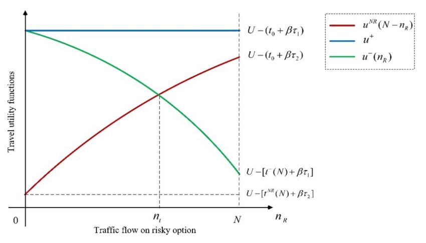
Sustainability 2021, 13, 3901                                                                                            3 of 24

                                reference [29]. Finally, decision makers’ preference reversals can be captured by the salience
                                theory, but not the prospect theory, which might be helpful to study travelers’ preference
                                reversals, e.g., [30]. Other differences between these two theories can be found in [31].
                                      Prospect theory and its extension, the cumulative prospect theory [32], have been
                                widely used in the studies on transportation and traffic (e.g., [28,29,33,34]). However, to
                                the best of our knowledge, only a few scholars discuss the effect of travelers’ salience
                                characteristic on the policy design and implementation, e.g., [35,36] studied the effect of
                                travelers’ salience characteristic on the pricing policy, which does not attract much attention
                                in transportation and traffic studies.
                                      Considering that the research on the effect of travelers’ salience characteristic is still
                                in its infancy, we focus on a stylized situation in this paper, where we consider travelers’
                                mode choice between two options (one risky option, i.e., the highway, and one non-risky
                                option, i.e., the transit) in the risky world with two state, and travel cost here refers to the
                                toll for the highway and fare for the transit. The motivation on this two-option choice
                                analysis is that travelers usually consider two modes in practice (e.g., [37,38]), while the
                                motivation for the two-state world assumption is the study in [39], where the authors point
                                out two flaws about the original salience theory. The first one is that, for some ranges of
                                probabilities, certainty equivalent is not defined, and the second one is that monotonicity is
                                violated by the model. We conjecture that these two flaws also exist in the flow-dependent
                                salience theory, an extension on the original salience theory, which is the foundation of our
                                analysis. Although we focus on the stylized situation, we make a thorough analysis on it
                                and obtain some novel results. The other contributions are summarized as follows.
                                      We propose a bi-attribute salient travel utility model with the continuous salience
                                ranking (also known as endogenous salience ranking), compared to the conventional
                                discrete ranking method proposed in [18]. Furthermore, we develop a bi-attribute salient
                                user equilibrium model based on this choice model and prove its solution existence and
                                uniqueness. Moreover, we analyze travelers’ risk attitudes in the bi-attribute mode choice
                                problem based on the equilibrium results. Finally, we conduct the numerical examples to
                                investigate the sensitivity of equilibrium solutions to the input parameters, which are cost
                                difference and salience bias, to shed light on travelers’ bi-attribute salient behavior. Our
                                findings provide insights into travelers’ behavioral studies related to the travel cost, which
                                can further provide implications for the policy design and implementation, especially on
                                the congestion tolling and transit fare design.
                                      The remainder of the paper is organized as follows. In Section 2, we present the basic
                                definitions and notations used in this paper. In Section 3, we propose the bi-attribute salient
                                travel utility model after introducing the flow-dependent salience theory. In Section 4, we
                                analyze the solution existence and uniqueness of the bi-attribute salient user equilibrium,
                                and based on this, we discuss travelers’ risk attitudes on the bi-attribute risky mode choice.
                                In Section 5, we conduct the numerical examples to show the performance of the proposed
                                model via the sensitivity analysis, followed by the conclusions and major findings in
                                Section 7.

                                2. Definitions and Notations
                                      We assume N travelers go from the common origin, e.g., the suburb area, to the
                                common destination, e.g., the core area, and study their bi-attribute (travel time and travel
                                cost) risky mode choice behavior with one risky option, i.e., the highway, denoted by R,
                                and one non-risky option, i.e., the transit, denoted by NR. Furthermore, we investigate
                                its long-run effect and assume there is no other mode options, e.g., staying at home. As
                                aforementioned, travelers mainly focus on these two travel modes in practice. There are
                                two states of the world, say good state and bad state, and the set of states is denoted by S.
                                We use p( p ∈ (0, 1)) to denote the probability of bad state and then 1− p is the probability
                                of good state. When p= 0 or p= 1, the risky option degenerates into a non-risky option,
                                which will not be discussed furthermore. On the non-risky option NR, the travel utility
                                functions are the same for both states, denoted by u NR , while the travel utility function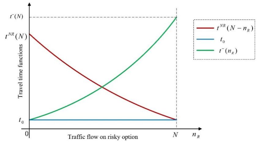
Sustainability 2021, 13, 3901                                                                                                4 of 24

                                on the risky option depends on the state, denoted by u+ in the good state, and u− in the
                                bad state.
                                     The nonlinear travel utility functions shown in Equation (1) are used in our study,
                                which are in the form of the difference between the utility value (due to the arrival at
                                the destination) U and the generalized cost (weighted sum of travel time and travel cost)
                                between the origin and the destination. Moreover, we assume that travelers could specify
                                a suitable value U to make the utility functions always positive as [28] and [40].

                                                         u+ (n R ) = U − [t0 + βτ1 ],
                                                         u− (n R ) = U − [t− (n R) + βτ1 ],                                    (1)
                                                         u NR ( N − n R ) = U − t NR ( N − n R ) + βτ2 ,


                                where n R denotes the traffic flows on the risky option, and then travel flows on the non-
                                risky option is N − n R . Travel costs on these two options, risky and non-risky option,
                                are τ1 and τ2 , respectively, and β > 0 denotes value of travel cost, which converts the
                                travel cost into travel time. At the same time, t− (n R ) and t NR ( N − n R ) are defined as
                                travel time functions on the risky option and the non-risky option, respectively. In this
                                paper, the travel time functions t− (n R ) and t NR ( N − n R ) are considered to be a continuous
                                strictly increasing function of the traffic volume on the corresponding option, and then
                                          dt− (n )          dt NR ( N −n )
                                we have dn R > 0 and
                                               R                dn R
                                                                     R
                                                                        < 0. In addition, it is assumed that t− ( N ) > t NR ( N ),
                                i.e., travel time of the risky option in bad state is larger than that of the non-risky option
                                when the flow is N, and the free flow travel times t0 on these two options are identical.
                                Therefore, the bad state is the most undesirable. Finally, the utility in the good state of the
                                risky option is a constant, which is normalized as U − (t0 + βτ1 ). Assumptions made here
                                could simplify our discussions in this paper, but our method can be extended accordingly
                                if some assumptions are relaxed, and nevertheless, the insights and implications obtained
                                according to our results will not be changed. The relationship between these travel time
                                functions is shown in Figure 1.

                                Figure 1. The relationship between the travel time functions.

                                3. Bi-Attribute Salient Travel Utility Model Based on Flow-Dependent
                                Salience Theory
                                     In this section, we introduce the flow-dependent salience theory first, and then propose
                                the bi-attribute salient route utility model based on this theory.

                                3.1. Flow-Dependent Salience Theory
                                      Following the principle of expected utility theory, the bi-attribute expected travel
                                utility on the risky option is (1 − p)u+ (n R ) + pu− (n R ), while the bi-attribute travel utility
                                on the non-risky option is u NR ( N − n R ). However, decision makers’ mind might focus
                                on whatever is odd, unusual or different, which is the essential meaning of salience
                                ([41]). Therefore, travelers could over-weight the route’s most salient states in S, and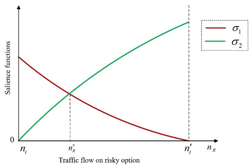
Sustainability 2021, 13, 3901                                                                                                     5 of 24

                                assign a subjective probability to each state s (good or bad state), which depends on the
                                objective probability of the state s and its salience. To formally define the flow-dependent
                                salience theory, let umax
                                                       s  and umin
                                                                s    denote the largest and smallest utilities for each state s,
                                                    − i
                                respectively, and us denote the utility of route j, j 6= s

                                Definition 1. The salience of state s for option i, i = R, NR, is a continuous and bounded
                                functionσ uis (n R ), u− i
                                                       s ( n R ) for a given flow n R that satisfies the following two conditions:
                                                                     s ∈ S we have that umin          (n R ), umax

                                1.    Ordering. If for states, e                                  s            s   (n R ) is a subset of
                                       min
                                       ues (n R ), uemax

                                                     s    (n R ) , then

                                                               σ uis (n R ), u− i            i
                                                                              s ( n R ) < σ ue
                                                                                                         −i
                                                                                             s ( n R ), ue
                                                                                                         s (n R )                    (2)

                                2.    Diminishing sensitivity. If uis (n R ) > 0 f or i = R, NR, then for any ε > 0,

                                                          σ uis (n R ) + ε, u− i                 i            −i
                                                                             s ( n R ) + ε < σ u s ( n R ), u s ( n R )              (3)

                                     In the original salience theory ([18]), there is another property for the salience function,
                                called reflection, which can handle negative utility. However, this property is not needed in
                                our study, because all the values of utility functions are positive. To illustrate Definition (1),
                                we use salience function
                                                                                    uis (n R ) − u− i
                                                                                                    s (n R )
                                                            σ uis (n R ), u− i
                                                                           s (n R ) =                                                (4)
                                                                                      uis (n R ) + u− i
                                                                                                    s (n R )

                                     It can be verified that this salience function satisfies both properties used in Defini-
                                tion (1). For a given value of n R , the ordering property shows that the difference between
                                the utility uis (n R ) of option u− i
                                                                  s ( n R ) of other option increases, and thus the salience of the
                                state s will increase, which is captured by uis (n R ) − u−      i
                                                                                               s ( n R ) . For a given value of n R , the
                                diminishing sensitivity property shows that if a state’s utility becomes larger, and thus the
                                salience will decrease, which is captured by uis (n R ) − u−         i
                                                                                                   s ( n R ). Moreover, we see that the
                                salience function (4) also satisfies the symmetry property, because we discuss the mode
                                choice between two options. Particularly, given states s, e            s ∈ S,state s is said tobe more
                                               s for option i (i = R, NR), if σ us (n R ), us (n R ) > σ ueis (n R ), ue−
                                                                                    i       − i                            i

                                salient than e                                                                           s (n R ) .
                                     We see that the travel utilities and the salience function are both flow-dependent,
                                where the flow denotes the traffic flow on the risky option, and thus, we call it flow-
                                dependent salience theory.

                                3.2. Bi-Attribute Salient Travel Utility Model
                                      Based on the flow-dependent salience theory, we propose the bi-attribute salient travel
                                utility model as follows.

                                Definition 2. According to the flow-dependent salience theory, travelers evaluate the bi-attribute
                                salient travel utility on the risky option according to the formulation

                                                                           δ1 (1 − p)u+ (n R ) + δ2 pu− (n R )
                                                            U R (n R ) =                                                             (5)
                                                                                   δ1 (1 − p) + δ2 p

                                while travelers evaluate the bi-attribute salient travel utility on the non-risky option according to
                                the formulation

                                                          δ1 (1 − p)u NR ( N − n R ) + δ2 pu NR ( N − n R )
                                          U NR (n R ) =                                                     = u NR ( N − n R )       (6)
                                                                         δ1 (1 − p) + δ2 p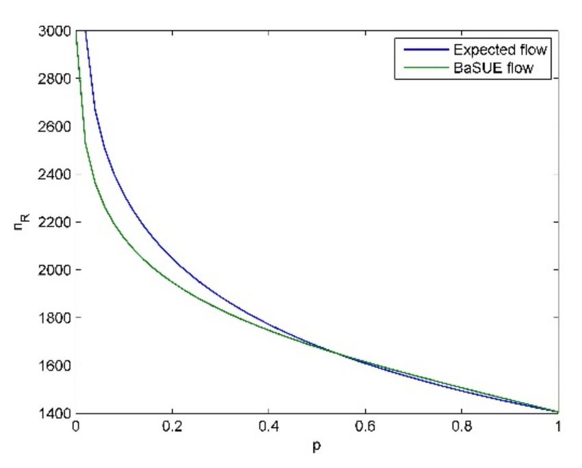
Sustainability 2021, 13, 3901                                                                                                              6 of 24

                                                   +       NR                                       − (n           NR ( N − n
                                where δ1 = δ−σ1 (u (nR ),u ( N −nR )) , and δ2 = δ−σ2 (u                   R ),u                R ))   .
                                    According to Equation (4), we have

                                                                                  |u+ (nR )−u NR ( N −nR )|
                                                                     σ1       =    u+ (n R )+u NR ( N −n R )
                                                                                                                                              (7)
                                                                                   |t NR ( N −nR )−t0 + β(τ2 −τ1 )|
                                                                              =   2U −t NR ( N −n R )−t0 − β(τ2 +τ1 )

                                                                              |u− (nR )−u NR ( N −nR )|
                                                                σ2        =    u− (n R )+u NR ( N −n R )
                                                                                                                                              (8)
                                                                               |t NR ( N −nR )−t− (nR )+ β(τ2 −τ1 )|
                                                                          =   2U −t NR ( N −n R )−t− (n R )− β(τ2 +τ1 )

                                      From Definition (2), we see that the bi-attribute salient travel utility on the risky
                                                                                                               δ p
                                option can be written as (1 − p0 )u+ (n R ) + p0 u− (n R ), where p0 = δ (1− 2p)+δ p , and the bi-
                                                                                                           1        2
                                attribute salient travel utility on the non-risky option remains the same, regardless of the
                                composition of the choice set. Compared to the formulation for the bi-attribute expected
                                utility theory, i.e., (1 − p)u+ (n R ) + pu− (n R ), we see that the only difference is the change
                                of the objective probability, which is called distorted probability for bad state and good
                                state based on flow-dependent salience theory.
                                      Parameter δ(δ ∈ (0, 1]) indicates travelers’ susceptibility to the salience, called salience
                                bias. δ = 1 means rational travelers, and thus there is no distortion on the objective
                                probabilities of the states. In the following study, when δ < 1, the travelers are called
                                salient travelers. Smaller value of δ means stronger salience bias, and vice versa. In the
                                special situation where δ → 0 , the salient travelers will only pay their attention on the
                                most bi-attribute salient travel utility.
                                      Based on the bi-attribute salient route utility presented in Definition (2), we obtain the
                                following proposition about the mode preference, which is basis of our equilibrium analysis.

                                Proposition 1. For a given flow n R , a salient traveler will choose the risky option if and only if the
                                following inequality satisfied.
                                                    h                            i       h                             i
                                          δ1 (1 − p) u+ (n R ) − u NR ( N − n R ) + δ2 p u− (n R ) − u NR ( N − n R ) > 0            (9)

                                Proof. For a given flow variable nR , based on the bi-attribute salient travel utility, a salient
                                traveler prefers the risky option to the non-risky option if and only if U R (nR ) > U NR (nR ) i.e.,

                                                       δ1 (1 − p)[u+ (n R ) + δ2 pu− (n R )]
                                                                                             > u NR ( N − n R )                             (10)
                                                                δ1 (1 − p) + δ2 p

                                Equation (9) can be obtained by Equation (10) after some rearrangement, which completes
                                the proof.

                                4. Bi-Attribute Salient User Equilibrium Analysis
                                     In this section, we study the long-run effect of bi-attribute salient travel utility, and
                                propose the bi-attribute salient user equilibrium (BaSUE), which can be stated as: No
                                traveler can improve their bi-attribute salient travel utility by unilaterally changing their options.
                                Furthermore, we compare the results of the BaSUE with those of bi-attribute expected
                                user equilibrium (BaEUE), which can be stated as: No traveler can improve their bi-attribute
                                expected travel utility by unilaterally changing their options.
                                     Based on Proposition (1), we see that at the BaSUE, the following equation is satisfied.
                                                     h                           i       h                           i
                                          δ1 (1 − p) u+ (n R ) − u NR ( N − n R ) + δ2 p u− (n R ) − u NR ( N − n R ) = 0        (11)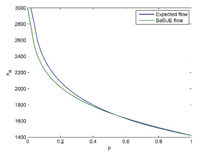
Sustainability 2021, 13, 3901                                                                                               7 of 24

                                    Furthermore, we define the following flow-dependent mode preference function based
                                on Equation (11), which is the foundation of our equilibrium analysis.

                                Definition 3. The flow-dependent mode preference function, denoted by VR→ NR (n R )is defined as
                                                           h                            i      h                            i
                                 VR→ NR (n R ) = δ1 (1 − p) u+ (n R ) − u NR ( N − n R ) + δ2 p u− (n R ) − u NR ( N − n R ) (12)

                                     From Definition (3), we see that when VR→ NR (n R ) > 0, the salient travelers prefer the
                                risky option to the non-risky option, when VR→ NR (n R ) < 0, the salient travelers prefer the
                                non-risky option to the risky option, and when VR→ NR (n R ) = 0, the BaSUE is reached.

                                4.1. Formal Results on the BaSUE
                                     Next, we present the formal analysis on the BaSUE, and before that, following the
                                principle of expected utility theory, we present the analysis on the BaEUE as a benchmark
                                case for comparison. We always use nRe to denote the equilibrium flow on the risky option.

                                Proposition 2. When − t NR ( N ) − t0 ≥ β(τ2 − τ1 ), there exists a corner BaEUE, where


                                nRe = 0, and when β(τ2 − τ1 ) ≥ p[t− ( N ) − t0 ], there exists a corner BaEUE, where nRe = N.

                                Proof. The proof can be completed based on the following logic. A corner BaEUE is
                                obtained when either of the following two conditions is satisfied.
                                1.   When nR = 0, the bi-attribute expected travel utility of the risky option is still not
                                     greater than the travel utility of the non-risky option, i.e., (1 − p)u+ (0) + pu− (0) ≤
                                     u NR ( N ). In this situation, we obtain that nRe = 0 is a corner BaEUE. Substitut-
                                     ing
                                        the travel utility   functions into this inequality and rearranging it, we obtain
                                     − t NR ( N ) − t0 ≥ β(τ2 − τ1 ).


                                2.   When nR = N, the bi-attribute expected travel utility of the risky option is still not less
                                     than the travel utility of the non-risky option, i.e., (1 − p)u+ ( N ) + pu− ( N ) ≤ u NR (0).
                                     In this situation, we obtain that nRe = N is a corner BaEUE. Substituting the travel
                                     utility functions into this inequality and rearranging it, we obtain p[t− ( N ) − t0 ] ≤
                                     β(τ2 − τ1 ).

                                      The intuitive interpretation on Proposition (2) is that when the travel cost of one
                                option is too large (or too small) compared to that of the other option, travelers’ mode
                                choice decisions cannot be changed, even though increase in traffic flow causes the increase
                                in travel time. That is, when the travel cost of a certain option is too large, no matter
                                how the traffic flow is distributed, travelers will choose the option with a small travel
                                cost, and vice versa.    According to this proposition, we only discuss the situations where
                                − t ( N ) − t0 < β(τ2 − τ1 ) < p[t− ( N ) − t0 ] is satisfied.
                                   NR

                                      Surprisingly, result in Proposition (2) is also a sound prerequisite for the analysis on
                                BaSUE due to the inherent relationship between the expected utility theory and salience
                                theory as discussed in the part of flow-dependent salience theory,     which will be elaborated
                                in the following discussions. We divide the condition − t NR ( N ) − t0 < β(τ2 − τ1 ) <


                                p[t− ( N ) − t0 ] into two cases, and the motivation for this division is the utility value when
                                the flow on each option is N.
                                1.   Case 1: 0 < β(τ2 − τ1 ) < p[t− ( N ) − t0 ]. In this case, the corresponding relationship
                                     between different travel utility functions is shown in Figure 2 schematically. We see
                                     that when the flow on each option is N, u+ ( N ) ≥ u NR ( N ) > u− ( N ) is satisfied. The
                                     relationship u+ ( N ) = u NR ( N ) when τ1 = τ2 is not shown explicitly, and one can
                                     modify Figure 2 for this straightforwardly. Moreover, relationship u+ ( N ) = u NR ( N )
                                     can also be
                                                incorporated  into Case 2 without loss of generality.
                                2.   Case 2: − t NR ( N ) − t0 < β(τ2 − τ1 ) < 0. In this case, the corresponding relationship
                                     between different travel utility functions is shown in Figure 3 schematically. We see
                                     that when the flow on each option is N, u NR ( N ) > u+ ( N ) > u− ( N ) is satisfied.
Sustainability 2021, 13, 3901                                                                                                     8 of 24

                                     Figure 2. Schematic relationship between different travel utility functions when τ1 ≤ τ2 .

                                     Figure 3. Schematic relationship between different travel utility functions when τ1 > τ2 .

                                          From Figures 2 and 3, we see that when nR ∈ [0, nt ] (here, nt denotes the tempo-
                                     rary value of n R , and is obtained by solving the equation u− (n R ) − u NR ( N − n R ) = 0),
                                     u+ (n R ) − u NR ( N − n R ) > 0 and u− (n R ) − u NR ( N − n R ) ≥ 0). Substituting these two
                                     inequalities into the flow-dependent mode preference function and with δ1 and δ2 being
                                     positive, we
                                                h have                    i        h                          i
                      VR→ NR(nR ) = δ1 (1 − p) u+ (n R ) − u NR ( N − n R ) + δ2 p u− (n R ) − u NR ( N − n R ) > 0                (13)

                                           i.e., the salient travelers always prefer the risky option to the non-risky option. There-
                                     fore, we obtain that when n R ∈ [0, nt ], there is no BaSUE. The aforementioned discussions
                                     are true for both cases, while for Case 2, we can obtain more results.
                                           When n R ∈ [n0 t , N ], N] (here, n0 t also denotes the temporary value of n R , and
                                     is obtained by solving the equation u+ (n R ) − u NR ( N − n R ) = 0), we have u+ (n R ) −
                                     u NR ( N − n R ) ≤ 0 and u− (n R ) − u NR ( N − n R ) < 0. Substituting these two inequalities
                                     into the flow-dependent mode preference function and with δ1 and δ2 being positive,
                                     we have h                               i      h                            i
                      VR→ NR(nR )   = δ1 (1 − p) u+ (n R ) − u NR ( N − n R ) + δ2 p u− (n R ) − u NR ( N − n R ) < 0            (14)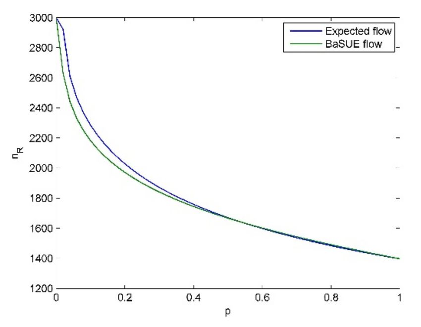
Sustainability 2021, 13, 3901 9 of 24
i.e., the salient travelers always prefer the non-risky option to the risky option. There-
fore, we obtain that when n R ∈ [n0 t , N ], there is no BaSUE. Therefore, in the following
discussions, we only consider interval (nt , N ] for Case 1, and interval (nt , n0 t ) for Case 2.
Next we discuss the BaSUE in these two cases separately based on the following
technical lemma.
Lemma 1. The flow-dependent mode preference function VR→ NR(nR ) is a strictly decreasing
function of the flow n R in the considered interval (nt , N ] or (nt , n0 t ).
Proof. We prove this lemma is true for interval (nt , n0 t ), and the proof for interval (nt , N ]
can be completed similarly, which is omitted for brevity.
It is obvious that in the interval (nt , n0 t ), VR→ NR(nR ) is continuous. The derivative of
VR→ NR(nR ) is
dVR→ NR(n ) dt NR ( N −nR ) i
h
dσ1 NR
dn R
R
= (1 − p)δ1 − ln δ dn R
t ( N − n R ) − t0 + β(τ2 − τ1 ) + dn R +
−
h NR i
dt ( N −n R )
dσ2 NR
t ( N − n R ) − t− (n R ) + β(τ2 − τ1 ) + − dt dn(nRR )
pδ2 − ln δ dn dn R
R
To prove the strict monotonicity of the flow-dependent mode preference function, the
t NR ( N −n R )−t0 + β(τ2 −τ1 )
following steps are followed. When n R (nt , n0 t )σ1 = 2U −t RN ( N −n R )−t0 − β(τ2 +τ1 )
, and thus
dt NR ( N −n R ) [U −( t
dσ1 dn R 0 + βτ1 )] dt NR ( N −n R )
dn R =2 2 . Because dn R < 0 and [U − (t0 + βτ1 )] > 0, we
[ 2U −t NR ( N −n R )− t0 − β ( τ2 + τ1 ) ]
dσ2
obtain dn R > 0.
t− (n R )−t NR ( N −n R )− β(τ2 −τ1 )
When n R (nt , n0 t ), σ1 = 2U −t RN ( N −n R )−t− (n R )− β(τ2 +τ1 )
, and thus
dt NR ( N −n R ) dt − (n )
dσ2 dn [U −(t− (nR )+ βτ1 )]− dn R [U −(t NR ( N −nR )+ βτ2 )]
dt ( N −n R ) NR
dn R = −2 R R
2 . Because dn R <
[2U −t NR ( N −nR )−t− (nR )− β(τ2 +τ1 )]
dt− (n R )
> 0, U − (t− (n R ) + βτ1 ) > 0, and U − t NR ( N − n R ) + βτ2 > 0, we obtain
0, dn R
dσ2
dn R> 0.
From Figure 3, we see that u+ (n R ) − u NR ( N − n R ) > 0,u− (n R ) − u NR ( N − n R ) < 0
when n R ∈ (nt , n0 t ), which can also be verified with the travel utility functions. There-
dσ1 dσ2
fore dn
R
= t NR ( N − n R ) − t0 + β(τ2 − τ1 ) < 0 and dn R
= t NR ( N − n R ) − t− (n R ) +
β(τ2 − τ1 ) < 0, δ ∈ (0, 1) implies ln δ < 0 and we have δ1 > 0 and δ2 > 0.
dVR→ NR(n )
Combining all these results, we can show that dn R
R
< 0, ∀n R ∈ (nt , n0 t ).
4.1.1. Case 1
In this case, 0 ≤ β(τ2 − τ1 ) < p[t− ( N ) − t0 ] is satisfied, which corresponds to Figure 2,
and we present the formal results on the equilibrium in this section.
The right-hand side of this inequality is the value when n R = N with the ob-
jective probability, which motivates us to discuss the value when n R = N with the
distorted probability.
When n R = N, one of three possible situations can happen given the specific travel util-
ity functions. If σ1 u+ ( N ), u NR (0) < σ2 u− ( N ), u NR (0) , i.e., badstate is salient (Recall
that δ ∈ (0, 1), δ1 > δ2 . Similarly, we obtain when σ1 u+ ( N ), u NR (0) > σ2 u− ( N ), u NR (0)
i.e., good state is salient, δ1 < δ2 , and when σ1 u+ ( N ), u NR (0) = σ2 u− ( N ), u NR (0) ,
i.e., no state is salient, δ1 = δ2 .
δ p δ p
If δ ∈ (0, 1), δ1 > δ2 , we have δ (1− 2p)+δ p < δ (1− 2p)+δ p = p i.e., the distorted
1 2 2 2
probability is strictly less than the objective probability. Similarly, if δ1 = δ2 , we have
δ2 p
δ1 (1− p)+δ2 p
= p, and if δ1 < δ2 , we have δ (1−δ2pp)+δ p > p.
1 2
Next, we discuss the three possible situations separately.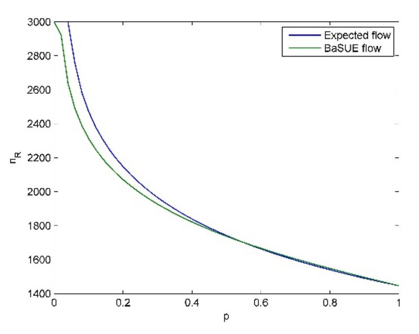
Sustainability 2021, 13, 3901                                                                                                 10 of 24

                                  Proposition 3. If δ1 > δ2 when n R = N, there is a unique BaSUE betweennt and N. In particular,
                                  the cost difference, which ensures that there is still no corner equilibrium, becomes smaller.

                                                                                                                δ p
                                  Proof. We complete the first part of the proof in two steps. When δ (1− 2p)+δ p [t− ( N ) − t0 ] <
                                                                                                           1       2
                                  β(τ2 − τ1 ), we have

       VR→ NR ( N ) = pδ2 t0 − t− ( N ) + β(τ2 − τ1 ) + (1 − p)δ1 [ β(τ2 − τ1 )]


                                 −               δ2 p       −                                    δ2 p      −
                   > pδ2 t0 − t ( N ) +                      t ( N ) − t0 + (1 − p)δ1                         t ( N ) − t0
                                          δ1 (1 − p) + δ2 p                                δ1 (1 − p) + δ2 p
                                                                                                                                (15)
                         δ1 (1 − p)[t0 − t− ( N )]

                                                                        δ2 p       −
                   = pδ2                           + (1 − p)δ1                      t ( N ) − t0
                             δ1 (1 − p) + δ2 p                   δ1 (1 − p) + δ2 p
                      =0

                                      Therefore, the salient travelers always prefer the risky option. That is, there is no
                                                   δ p
                                  BaSUE when δ (1− 2p)+δ p [t− ( N ) − t0 ] < β(τ2 − τ1 ) < p(t− ( N ) − t0 ).
                                                  1         2
                                                                       δ2 p
                                       When 0 ≤ β(τ2 − τ1 ) ≤    δ1 (1− p)+δ2 p
                                                                                [t− ( N ) − t0 ], there is a unique BaSUE between nt
                                                                          δ p
                                  and N. It can be verified that δ (1− 2p)+δ p [t− ( N ) − t0 ] = β(τ2 − τ1 ), i.e., VR→ NR ( N ) = 0.
                                                                     1          2
                                                                                                                dV     (n )
                                  Following the similar steps used in the proof of Lemma (1), we obtain R→dnNR R < 0, ∀n R ∈
                                                                                                                     R
                                 (nt , N ). Combining the results that VR→ NR (nt ) > 0 and VR→ NR ( N ) ≤ 0, we can show that
                                 there is a unique value of n R ∈ (nt , N ] that satisfies VR→ NR (nRe ) = 0, which completes the
                                 first part of the proof.
                                                     δ p
                                       Finally, δ (1− 2p)+δ p < p means that the cost difference, which ensures that there is still
                                                 1         2
                                 no corner equilibrium, becomes smaller.

                                  Proposition 4. If δ1 = δ2 when n R = N, there is a unique BaSUE between nt and N. In
                                  particular, the cost difference, which ensures that there is still no corner equilibrium, remains
                                  the same.

                                  Proof. If δ1 = δ2 when n R = N, the BaSUE becomes the BaEUE. Follow the aforemen-
                                                                dV      (n )
                                  tioned discussions, we have R→dnNR R < 0, ∀n R ∈ (nt , N ). Combining the results that
                                                                      R
                                  VR→ NR (nt ) > 0 and VR→ NR ( N ) ≤ 0, we complete the first part of the proof.

                                                      δ p
                                       Finally, δ (1− 2p)+δ p = p means that the cost difference, which ensures that there is still
                                                 1         2
                                  no corner equilibrium, remains the same.

                                  Proposition 5. If δ1 < δ2 when n R = N, there is a unique BaSUE between nt and N. In
                                  particular, we can increase the cost difference, and meanwhile, guarantee that there is still no
                                  corner equilibrium.

                                  Proof. If δ1 < δ2 when n R = N, we have

                                                                                            δ2 p
                                                  β(τ2 − τ1 ) < p t− ( N ) − t0 <
                                                                                                     −
                                                                                                        t ( N ) − t0
                                                                                     δ1 (1 − p) + δ2 p

                                                                                                 dV      (n )
                                       Follow the aforementioned discussions, we have R→dnNR R < 0, ∀n R ∈ (nt , N ).
                                                                                                  R
                                  Combining the results that VR→ NR (nt ) > 0 and VR→ NR ( N ) ≤ 0, we complete the first part
                                  of the proof.

                                                      δ p
                                      Finally, δ (1− 2p)+δ p > p means that we can increase the cost difference, and meanwhile,
                                                1         2
                                  guarantee that there is still no corner equilibrium.
Sustainability 2021, 13, 3901 11 of 24
All the results in the above three propositions about the corner equilibrium can be
verified with the logic discussed in Proposition (2), by replacing the objective probability p
with the distorted probability p0 .
4.1.2. Case 2
In this case, − t NR ( N ) − t0 < β(τ2 − τ1 ) < 0 is satisfied, which corresponds to
Figure 3, and we present the formal results on the equilibrium in this section. In this case,
there is no objective probability p on left-hand side of the inequality, which is different from
that in Case 1.
Proposition 6. There is a unique BaSUE nRe between nt and n0 t .
Proof. VR→ NR(nt ) = δ1 (1 − p) u+ (nt ) − u NR ( N − nt ) > 0, VR→ NR (n0 t ) = δ2 p[u− (n0 t )−
u NR ( N − n0 t ) < 0, combining these results in Lemma (1), we obtain that there is a unique
value of n R ∈ (nt , n0 t ) hat satisfies VR→ NR (nRe ) = 0, which completes the proof.
4.2. Travelers’ Risk Attitude on the Bi-Attribute Risky Mode Choice
In this section, we present the results on travelers’ attitude based on the BaSUE.
Theorem 1. At the equilibrium, if no state is salient, i.e., δ1 = δ2 , travelers are risk-neutral; if good
state is salient, i.e., δ1 < δ2 , travelers are risk-seeking; if bad state is salient, i.e., δ1 > δ2 , travelers
are risk-averse.
Proof. At the BaSUE, − if no state is salient, we have δ1 = δ2 , and thus Equation (13)
NR ( n ) + (1 − p ) δ u+ ( n ) − u NR ( n ) = 0. Then we
becomes pδ 1 ( 1 − p ) u ( n R ) − u R 1 R R
have p u− (n R ) − u NR (n R ) + (1 − p) u+ (n R ) − u NR (n R ) = 0, i.e.,
pu− (n R ) + (1 − p)u+ (n R ) = 0 (16)
Therefore, we obtain the BaEUE. The distorted probability of good state will become larger
if it is salient, which will increase the left-hand-side value of Equation (16). Therefore, more
travelers will choose the risky option, i.e., they are risk-seeking. Similarly, the distorted
probability of the bad state will become larger if it is salient, which will decrease the
left-hand-side value of Equation (16). Therefore, more travelers will choose the non-risky
option, i.e., they are risk-averse.
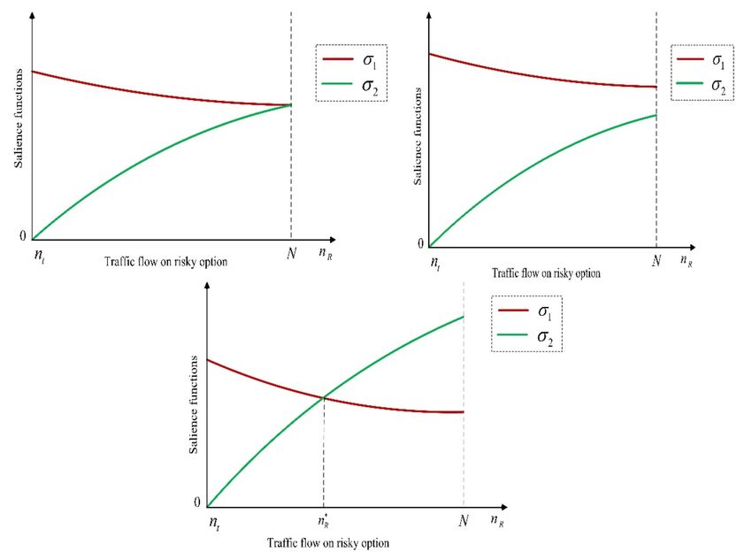
In practice, maybe only one state is salient for a specific situation, as shown in the fol-
lowing Figure 4. Next, we propose the flow-dependent salience ranking analysis to present
more detailed results based on Theorem (1), and obtain the following two propositions.
Result in Proposition (7) is motivated by the discussion on the BaSUE in Case 1, where the
relationship between δ1 and δ2 is a key prerequisite when n R = N. Here, we discuss the
conditions for this relationship.Sustainability 2021, 13, 3901 12 of 24
Figure 4. Relationship between different salience functions.
β(τ −τ ) t− ( N )−t0 − β(τ2 −τ1 )
When n R = N, we have σ1 = 2U −2t −2 β(τ1 +τ ) and σ2 = 2U −t0 −t− ( N )− β(τ2 +τ1 )
. If
0 2 1
σ1 < (=, >)σ2 (see Figure 4), we obtain
β(τ2 − τ1 ) t− ( N ) − t0 − β(τ2 − τ1 )
< (=, >) (17)
2U − 2t0 − β(τ2 + τ1 ) 2U − t0 − t− ( N ) − β(τ2 + τ1 )
Equation (17) can be seen as the sufficient conditions to figure out the salient state
when n R = N.
With the sufficient conditions, we obtain the following proposition.
Proposition 7. In the case that 0 ≤ β(τ2 − τ1 ) < p(t− ( N ) − t0 ), one of the following three
situations can happen given the travel utility functions.
1. σ1 ( N ) < σ2 ( N )is satisfied, and then we can find ann∗R ∈ (nt , N ). Whenn R ∈ (nt , n∗R ),σ1 >
σ2 , i.e., good state is salient and travelers are risk-seeking; whenn R ∈ (n∗R , N ),σ2 > σ1 , i.e.,
bad state is salient and travelers are risk-averse; whenn R = n∗R , σ1 = σ2 , i.e., no state is
salient and travelers are risk-neutral.
2. σ1 ( N ) = σ2 ( N )is satisfied, and then when n R ∈ (nt , N ), σ1 > σ2 , i.e., good state is salient
and travelers are risk-seeking, and when n R = N, σ1 = σ2 , i.e., no state is salient and
travelers are risk-neutral.
3. σ1 ( N ) > σ2 ( N )is satisfied, and then whenn R ∈ (nt , N ], σ1 > σ2 , i.e., good state is salient
and travelers are risk-seeking.
Proof. According to the aforementioned discussions in Lemma (1), σ1 (n R ) and σ2 (n R ) are
dσ1
both continuous functions of n R . dn < 0, ∀n R ∈ (nt , N ], i.e., σ1 is a strictly decreasing
R
dσ2
function of n R when n R ∈ (nt , N ], and dn > 0, ∀n R ∈ (nt , N ], i.e.,σ2 is a strictly increasing
R
function of n R when n R ∈ (nt , N ] We have discussed the relationship between σ1 and σ2
when n R = N. With the strict monotonicity properties, we need to figure out the relation-
ship between σ1 and σ2 when n R = nt . Recalling that nt is obtained by solving the equationSustainability 2021, 13, 3901 13 of 24
u− (n R ) − u NR ( N − n R ) = 0, we have σ2 (nt ) = 0 and σ1 (nt ) > 0 by Equations (7) and (8).
Therefore, combining all the results, we obtain the following three possible situations.
(a) σ1 ( N ) < σ2 ( N ) as schematically shown in the upper-left figure of Figure 4. Then
there exists n∗R ∈ (nt , N ). When n R ∈ (nt , n∗R ), σ1 > σ2 , when n R ∈ (n∗R , N ), σ2 > σ1 ,
when n R = n∗R , σ2 = σ1 .
(b) σ1 ( N ) = σ2 ( N ) as schematically shown in the upper-right figure of Figure 4. When
n R ∈ (nt , N )σ1 > σ2 and when n R = N, σ1 = σ2 .
(c) σ1 ( N ) > σ2 ( N ) as schematically shown in the bottom figure of Figure 4. When
n R ∈ (nt , N ], σ1 > σ2 . Combining with the results in Theorem (1), we complete
the proof.
Next, we talk about another case, i.e., Case 2.
Proposition 8. In the case that − t NR ( N ) − t0 < β(τ2 − τ1 ) < 0, we can find an n∗R ∈
(nt , n0 t ). When n R ∈ (nt , n∗R ), σ1 > σ2 , i.e., good state is salient and travelers are risk-seeking;
when n R ∈ (n∗R , n0 ), σ2 > σ1 , i.e., bad state is salient and travelers are risk-averse; when
n R = n∗R , σ1 = σ2 , i.e., no state is salient and travelers are risk-neutral.
Proof. It is obvious that in the interval (nt , n0 t ), σ1 (n R ) and σ2 (n R ) are both continuous func-
t NR ( N −n R )−t0 + β(τ2 −τ1 ) t− (n )−t NR ( N −n )− β(τ −τ )
tions of n R . We have σ1 = ,σ = 2U −t NRR ( N −n )−t−R(n )− β2(τ +1 τ ) ,
2U −t NR ( N −n R )−t0 − β(τ2 +τ1 ) 2 R R 2 1
dσ1
when n R ∈ (nt , n0 t ). According to Lemma (1), dn < 0, ∀n R ∈ (nt , n0 t ),i.e.,σ1 is a strictly
R
dσ2
decreasing function of n R when n R ∈ (nt , n0 t ), and dn > 0, ∀n R ∈ (nt , n0 t ), i.e., σ2 is a
R
0
strictly increasing function of n R when n R ∈ (nt , n t ). Moreover, when n R = nt , we have
σ2 (nt ) = 0 and σ1 (nt ) > 0; when n R = n0 t , σ2 (n0 t ) = 0 and σ1 (n0 t ) = 0, recalling the
calculation of n0 t . Therefore, there is a value between nt and n0 t , defined as n∗R , that σ1 = σ2 ,
as schematically shown in Figure 5. Furthermore, when n R ∈ (nt , n∗R ), σ1 > σ2 ; when
n R ∈ (n∗R , n0 t ), σ2 > σ1 . Combining with the results in Theorem (1), we complete the proof.
Figure 5. Relationship between different salience functions.
5. Numerical Examples
In this section, we conduct the numerical examples to show the performance of
the proposed method, focusing on the sensitivity of equilibrium solution to the inputSustainability 2021, 13, 3901 14 of 24
parameters, the cost difference and the salience bias. We assume that there are N = 3000
travelers in the system, and use the following quadratic travel utility functions.
2 !
f
u = U − t0 + at0 + βτ (18)
Q
where f denotes the traffic flow, Q denotes the capacity, t0 denotes the free-flow travel
time, and parameters a = 0.15. The free-flow travel times on both options are 80, and the
capacity of risky option and non-risky option are 1000 and 1200, respectively. The intrinsic
value U is 205, and the value of travel cost β is 0.5. We change the value of p from 0 to
1, and use the linspace function in Matlab to generate 51 representative values. All the
flow-dependent mode choice functions are solved with solve function in Matlab 2014a. We
run the numerical examples for each case.
6. Case 1
In this case, 0 ≤ β(τ2 − τ1 ) < p(t− ( N ) − t0 ) is satisfied. The travel cost on the risky
option is 20, while the travel cost on the non-risky option is increased from 21 to 30 with the
step size being 3. That is, we choose four representative values for travel cost on non-risky
option. The salience bias δ is 0.3. The final equilibrium results are shown in Tables 1–4
(here we select 17 representative values for p) and Figures 6–9.
Table 1. Comparison of the equilibrium flow for representative values of p(τ1 = 20 and τ2 = 21).
p 0.02 0.08 0.14 0.20 0.26 0.32 0.38 0.44 0.50
Expected flow 2627 2270 2093 1971 1878 1802 1738 1683 1635
BaSUE flow 2500 2177 2025 1921 1843 1778 1723 1675 1632
p 0.56 0.62 0.68 0.74 0.80 0.86 0.92 0.98 -
Expected flow 1592 1553 1518 1486 1456 1429 1403 1379 -
BaSUE flow 1593 1557 1524 1492 1463 1434 1407 1380 -
Table 2. Comparison of the equilibrium flow for representative values of p(τ1 = 20 and τ2 = 24).
p 0.02 0.08 0.14 0.20 0.26 0.32 0.38 0.44 0.50
Expected flow 2923 2364 2162 2028 1927 1846 1779 1721 1670
BaSUE flow 2631 2247 2081 1971 1887 1820 1762 1721 1667
p 0.56 0.62 0.68 0.74 0.80 0.86 0.92 0.98 -
Expected flow 1625 1585 1548 1515 1484 1456 1429 1405 -
BaSUE flow 1627 1589 1554 1522 1491 1462 1433 1406 -
Table 3. Comparison of the equilibrium flow for representative values of p(τ1 = 20 and τ2 = 27).
p 0.02 0.08 0.14 0.20 0.26 0.32 0.38 0.44 0.50
Expected flow 3000 2469 2234 2081 1978 1892 1820 1759 1706
BaSUE flow 2775 2318 2138 2021 1933 1861 1801 1749 1702
p 0.56 0.62 0.68 0.74 0.80 0.86 0.92 0.98 -
Expected flow 1659 1617 1579 1544 1512 1483 1455 1430 -
BaSUE flow 1660 1621 1585 1551 1519 1489 1460 1431 -
Table 4. Comparison of the equilibrium flow for representative values of p(τ1 = 20 and τ2 = 30).
p 0.02 0.08 0.14 0.20 0.26 0.32 0.38 0.44 0.50
Expected flow 3000 2587 2310 2147 2029 1937 1862 1797 1742
BaSUE flow 2923 2391 2196 2071 1978 1903 1840 1786 1737
p 0.56 0.62 0.68 0.74 0.80 0.86 0.92 0.98 -
Expected flow 1692 1649 1609 1573 1540 1510 1481 1455 -
BaSUE flow 1694 1653 1616 1581 1548 1516 1486 1456 -Sustainability 2021, 13, 3901 15 of 24
Figure 6. τ1 = 20 and τ2 = 21.
Figure 7. τ1 = 20 and τ2 = 24.
Figure 8. τ1 = 20 and τ2 = 27.
Figure 9. τ1 = 20 and τ2 = 30.Sustainability 2021, 13, 3901 16 of 24
Before we discuss the main insights of the results, we present four common aspects
in all the testings. (1) In our testing, the sufficient condition σ1 ( N ) < σ2 ( N ) is satisfied,
i.e., the relationship between σ1 and σ2 are shown in the upper-left figure of Figure 4. One
can modify the travel utility func-tions to test other two situations; (2) In all the following
figures, we claim that the cross point (denoted by neR ) of the two curves, the curve for
expected flow following the principle of expected utility theory and the curve for BaSUE
flow following the principle of flow-dependent salience theory, is a special situation, where
travelers are risk-neutral according to Theorem (1). The condition, that the solution to the
flow-dependent mode choice function and the solution to the equation σ1 (n R ) < σ2 (n R )
coincide, needs to be satisfied, which can be verified by the related definitions. The above
condition can also be used to figure out the Pe of the bad state when travelers are risk-
neutral. (3) When p = 0 or p = 1,we obtain the degeneration values for the equilibrium
solution. In both cases, when p = 0, the solution is obtained by solving the equation
u+ (n R ) = u NR ( N − n R ), and when p = 1, the solution is obtained by solving the equation
u− (n R ) = u NR ( N − n R ), given the specific values of τ1 and τ2 . (4) In all the testings, we
can always find the unique BaSUE solution, which demonstrates Proposition (3).
From these tables and figures, we see the following insights.
(1) Given a specific objective probability (e.g., p = 0.2), when the cost difference (cost
difference here means τ2 − τ1 ) become larger and larger, traffic flow on the risky
option will become larger and larger, and vice versa. The intuitive explanation for
this is that the increase of travel cost on non-risky option will make travelers choose
the risky option.
(2) When the probability of bad state is not large (e.g., p = 0.2), travelers are risk-averse,
and when the probability of bad state is relatively large (e.g., p = 0.7), travelers are
risk-seeking. We also see the cross point and its corresponding pe, where travelers
are risk-neutral as discussed before. For p ∈ (0, pe), travelers are risk averse, and for
p ∈ ( pe, 1), travelers are risk-seeking. These results seem to be non-intuitive, and it
seems that if the travelers know that the risky option is in bad state (in good state)
with high probability, they should choose the non-risky (risky) option, i.e., they should
be risk-averse (risk-seeking). However, travelers’ salience characteristic means they
put their attention on the unusual aspect. That is, if the risky option is in bad state (in
good state) with high probability, considering the low (high) flow on the risky option
(see Figures 6–9), the good state (the bad state) is the unusual aspect according to our
travel utility functions. Moreover, we can combine the results in Proposition (7) to
present more interpretation on these phenomena. When the probability of bad state
is not large, the equilibrium solution nRe is larger than ncR , and thus, we know bad
state is salient according to Proposition (7). In contrast, we know good state is salient
when the probability of bad state is large. Therefore, we see these phenomena in the
testings. All the above discussions also demonstrate the validity of Theorem (1).
(3) When the cost difference become larger and larger, the extent of travelers’ risk-averse
attitude becomes stronger almost, except when p is very small, e.g., p = 0.02. This
is because larger cost difference will make travelers choose the risky option, which
further makes the difference between travel utility of risky option in good state and
the travel utility of non-risky option become smaller, considering the high flow on the
risky option (see Figures 6–9). Therefore, the bad state is more salient, which leads
to the stronger extent of travelers’ risk-averse attitude. However, there is almost no
difference between the risk-neutral equilibrium flow, i.e., the expected flow, and the
risk-seeking equilibrium flow, i.e., the BaSUE flow when p is relatively large. That
is, travelers’ risk-seeking attitude following the flow-dependent salience theory has
almost no effect on the equilibrium flow, compared to the results of expected utility
theory. This is because the flow on the risky option is not large (see Figures 6–9),
which make the difference between the utilities on risky and non-risky option small.
(4) With the increase of cost difference, we clearly see the corner equilibrium following
the principle of expected utility theory. Meanwhile, larger cost difference means moreSustainability 2021, 13, 3901 17 of 24
situations with corner equilibrium. However, there is no corner equilibrium for BaSUE
even though we increase the cost difference, which demonstrate Proposition (5).
Next, we fix the travel cost on the risky option (τ1 = 20) and non-risky option (τ1 = 25),
and change the values of salience bias δ. We choose four representative values for δ, which
are 0.1, 0.3, 0.5 and 0.7. δ = 0.1 implies that travelers have stronger salience bias, while
δ = 0.7 implies the salience bias is weaker. The final equilibrium results are shown in
Figures 10–13. From these figures, we see the following insights. (1) With the increase
of the value for δ, the extent of travelers’ risk-averse attitude and risk-seeking attitude
become weaker, and vice versa. (2) The value of δ has no effect on the cross point, where
travelers are risk-neutral, as discussed before. (3) We clearly see the values for p, where
there exists the corner equilibrium for expected flow, and the value of δ has no effect on this.
(4) Even though travelers have very strong salience bias, e.g., δ = 0.1, the effect of travelers’
risk-seeking attitude following the flow-dependent salience theory on the equilibrium
results can be ignored, compared to the results of expected utility theory. We can present
similar explanations as the above testing.
Figure 10. δ = 0.1.
Figure 11. δ = 0.3.Sustainability 2021, 13, 3901 18 of 24
Figure 12. δ = 0.5.
Figure 13. δ = 0.7.
6.1. Case 2
In this case, − t NR ( N ) − t0 < β(τ2 − τ1 ) < 0 is satisfied. The travel cost on the
non-risky option is 20, while the cost on the risky option is increased from 21 to 30 with
the step size being 3. That is, we choose four representative values for travel cost on risky
option. The salience bias δ is also 0.3. The final equilibrium results are shown in Tables 5–8
(here we also select 17 representative values for p) and Figures 14–17.
Table 5. Comparison of the equilibrium flow for representative values of p(τ1 = 21 and τ2 = 20).
p 0.02 0.08 0.14 0.20 0.26 0.32 0.38 0.44 0.50
Expected flow 2509 2211 2048 1934 1845 1772 1711 1658 1611
BaSUE flow 2419 2130 1987 1888 1813 1750 1697 1650 1609
p 0.56 0.62 0.68 0.74 0.80 0.86 0.92 0.98 -
Expected flow 1570 1532 1498 1467 1438 1411 1386 1363 -
BaSUE flow 1571 1536 1503 1473 1444 1416 1389 1364 -
Table 6. Comparison of the equilibrium flow for representative values of p(τ1 = 24and τ2 = 20).
p 0.02 0.08 0.14 0.20 0.26 0.32 0.38 0.44 0.50
Expected flow 2367 2127 1984 1879 1797 1729 1671 1620 1576
BaSUE flow 2308 2062 1931 1839 1768 1709 1658 1614 1574
p 0.56 0.62 0.68 0.74 0.80 0.86 0.92 0.98 -
Expected flow 1536 1500 1468 1437 1410 1384 1360 1337 -
BaSUE flow 1537 1504 1473 1443 1415 1389 1363 1338 -Sustainability 2021, 13, 3901 19 of 24
Table 7. Comparison of the equilibrium flow for representative values of p(τ1 = 27 and τ2 = 20).
p 0.02 0.08 0.14 0.20 0.26 0.32 0.38 0.44 0.50
Expected flow 2248 2049 1921 1825 1749 1685 1631 1583 1541
BaSUE flow 2207 1995 1876 1790 1723 1667 1619 1577 1539
p 0.56 0.62 0.68 0.74 0.80 0.86 0.92 0.98 -
Expected flow 1503 1469 1437 1408 1382 1357 1334 1312 -
BaSUE flow 1504 1472 1442 1414 1387 1361 1337 1313 -
Table 8. Comparison of the equilibrium flow for representative values of p(τ1 = 30 and τ2 = 20).
p 0.02 0.08 0.14 0.20 0.26 0.32 0.38 0.44 0.50
Expected flow 2144 1976 1861 1773 1702 1642 1591 1546 1506
BaSUE flow 2114 1931 1822 1742 1679 1626 1581 1540 1504
p 0.56 0.62 0.68 0.74 0.80 0.86 0.92 0.98 -
Expected flow 1470 1437 1407 1379 1354 1330 1308 1287 -
BaSUE flow 1471 1440 1411 1384 1359 1334 1310 1288 -
Figure 14. τ1 = 21 and τ2 = 20.
Figure 15. τ1 = 24 and τ2 = 20.Sustainability 2021, 13, 3901 20 of 24
Figure 16. τ1 = 27 and τ2 = 20.
Figure 17. τ1 = 30 and τ2 = 20.
From these tables and figures, we see the following insights. (1) Given a specific value
of objective probability (e.g., p = 0.2), when the cost difference (cost difference here means
τ1 − τ2 ) becomes larger and larger, traffic flow on the risky option will become smaller and
smaller, and vice versa. The intuitive explanation for this is that the increase of travel cost
on risky option will make travelers choose the non-risky option. (2) We also see travelers’
risk-seeking and risk-averse attitudes for different objective probability ps, and can give
similar explanations as those in Case 1. Also, the risk-neutral attitude is a special condition.
(3) When the cost difference become larger and larger, the extent of travelers’ risk-averse
attitude almost remains the same, even though it becomes weaker. Increase in the cost
difference will make more travelers choose non-risky option, and the difference between the
utility of the risky option in good state and the utility of the non-risky option become larger.
Meanwhile, increase of the value of τ1 makes this difference become smaller. Therefore, this
difference remains almost the same, and we see this phenomenon on travelers’ risk-averse
attitude. Similarly, there is almost no difference between the expected flow, and the BaSUE
flow when travelers’ are risk-seeking, and we can present similar explanation as those
in Case 1. (4) In this test, there is no corner equilibrium for both principles, and one can
modify the travel utility functions and travel costs to show the corner equilibrium.
Next, we fix the travel cost on the risky option (τ1 = 25) and non-risky option (τ2 = 20),
and change the values of salience bias δ. We also choose four different value for δ, which
are 0.1, 0.3, 0.5 and 0.7. The final equilibrium results are shown in Figures 18–21. From
these figures, we see the similar behavioral insights as the tests shown from Figures 10–13.You can also read