Versatile total angular momentum generation using cascaded J-plates
←
→
Page content transcription
If your browser does not render page correctly, please read the page content below
Vol. 27, No. 5 | 4 Mar 2019 | OPTICS EXPRESS 7469

Versatile total angular momentum generation
using cascaded J-plates
YAO -W EI H UANG , 1,2 N OAH A. R UBIN , 1 A NTONIO A MBROSIO, 3
Z HUJUN S HI , 1,4 R OBERT C. D EVLIN , 1,5 C HENG -W EI Q IU , 2 AND
F EDERICO C APASSO 1,*
1 Harvard  John A. Paulson School of Engineering and Applied Sciences, Harvard University, Cambridge,
MA 02138, USA
2 Department of Electrical and Computer Engineering, National University of Singapore, Singapore
117583, Singapore
3 Center for Nanoscale Systems, Harvard University, Cambridge, MA 02138, USA
4 Department of Physics, Harvard University, Cambridge, MA 02138, USA
5 Metalenz, Weston, MA 02493, USA
* capasso@seas.harvard.edu

Abstract: Optical elements coupling the spin and orbital angular momentum (SAM/OAM) of
light have found a range of applications in classical and quantum optics. The J-plate, with J
referring to the photon’s total angular momentum (TAM), is a metasurface device that imparts two
arbitrary OAM states on an arbitrary orthogonal basis of spin states. We demonstrate that when
these J-plates are cascaded in series, they can generate several single quantum number beams
and versatile superpositions thereof. Moreover, in contrast to previous spin-orbit-converters, the
output polarization states of cascaded J-plates are not constrained to be the conjugate of the input
states. Cascaded J-plates are also demonstrated to produce vector vortex beams and complex
structured light, providing new ways to control TAM states of light.
© 2019 Optical Society of America under the terms of the OSA Open Access Publishing Agreement

1.   Introduction
In 1909, Poynting realized that circularly polarized light carries angular momentum [1] that is
now known as spin angular momentum (SAM) [2]. A beam’s SAM carries a value of S = σ~
per photon, where σ is ±1. Orbital angular momentum (OAM), however, is independent of the
beam’s polarization. It arises from its helical phase front. The Laguerre-Gaussian modes have
been widely used in laser cavities [3, 4] and optical vortices [5]. It took until 1992, however,
for Allen et al. to point out that these beams with the azimuthal phase ei`φ carry an OAM of
L = `~ per photon, where ` is an integer [6]. These beams have a phase singularity on axis,
while the Poynting vector spirals around it. This results in annular intensity profile and spiral
interference pattern obtained upon interference with a reference beam of uniform phase. The
beam’s total angular momentum (TAM)—in the paraxial approximation—is a sum of the spin
and orbital contributions J = (` + σ)~ per photon. The electromagnetic field has a well-defined
total angular momentum J, but the separation specifically into spin and angular components is
one of convenience and is not unique, rigorously speaking [7]. While it is inherently difficult
to measure the SAM and OAM of a single photon, doing so for a beam is straightforward. We
can measure the spin with quarter-wave plate and polarizer and the OAM quantum number by
observing the number of arms in the aforementioned interference pattern.
   There are many methods to generate OAM-carrying beams in free space [6,8–10] and as surface
waves [11, 12], and many applications have been demonstrated, such as optical tweezers [13],
optical communication [14–16], quantum entanglement [17–19], super-resolution imaging [20],
quantum memory [21], lasers and microlasers [22, 23], OAM-molecule interaction [24], etc.
In many of these schemes, the incident beam’s polarization has no relation to the OAM of
the generated beam. In a class of devices known as spin-orbit converters, however, the output

#356118                                                                   https://doi.org/10.1364/OE.27.007469
Journal © 2019          Received 28 Dec 2018; revised 16 Feb 2019; accepted 16 Feb 2019; published 27 Feb 2019
Vol. 27, No. 5 | 4 Mar 2019 | OPTICS EXPRESS 7470

OAM state depends explicitly on the polarization of incoming light. One such device, known
as a Q-plate, is one of the common methods used to generate OAM beams by spin-to-orbital
conversion [25,26]. Q-plates mainly refer to the implementation realized using liquid crystals, e.g.
special light modulator (SLM) that allow producing dynamical diffraction patterns [22,26], but the
relatively large pixel size limits the beam quality and efficiency. Dielectric metasurfaces composed
of sub-wavelength artificial structures enable spatial modulations of phase and polarization on
demand [27]. This enables high-efficiency spin-orbital conversion and vortex beams with high
and even fractional topological charges [28, 29]. Regardless of their particular implementation,
Q-plate devices have two restrictions inherent in their construction. First, they operate on a
circular polarization basis (|Ri or |Li). Second, the output OAM states corresponding to these
circular polarizations are constrained to hold conjugate (equal and opposite) values (` and −`).
Here, we use two kets to describe spin and orbital states in Fig. 1. A schematic of a Q-plate is
shown in Fig. 1(a).
    Recently, designs utilizing independent phase control of two arbitrary orthogonal polarizations
have been shown to overcome these restrictions [30, 31]. Previous works demonstrated non-
conjugate OAM beams [30] and hologram images [31] imparted in the circular polarization basis,
overcoming the second restriction stated above. The first restriction was recently overcome in
the form of the J-plate, a metasurface device that may impart two arbitrarily specified helical
phase fronts on two arbitrary orthogonal spin states (Fig. 1(b)) [32]. That is, the two possible
output orbital states |mi and |ni can be independent. This cannot be achieved with Q-plates or
with SLMs. The name J-plate refers to the variable denoting the photon’s TAM. However, one
restriction remains: The output polarization states must be the same states as the input states
with flipped handedness (|(λ+ )∗ i and |(λ− )∗ i) if a single layer of metasurface elements with only
linear structural birefringence is used [30–32].
    In this work, we develop the notion of cascaded J-plates, that is, two J-plates placed after
another in series. These cascaded J-plates may generate versatile TAM states, notably without the
aforementioned restriction in [32]. That is, the output polarization states can be another arbitrary
orthogonal polarization basis (|κ + i and |κ − i) independent of input polarization basis (|λ+ i and
|λ− i) (Fig. 1(c)). The number of J-plates cascaded is not limited to just two. We demonstrate two
and the method can extend to more than two. Figure 2(a) illustrates the concept of a cascaded
two J-plate system. When the incident polarization state |Ψi i passes through the first J-plate
(represented by the Jones matrix operator J1 ), J1 |Ψi i emerges. The state J1 |Ψi i could be one
of the two design OAM states or a superposition. We assume that the second J-plate (J2 ) has
different eigen-polarization states than the first J-plate. After J1 |Ψi i passes through the second
J-plate, J2 J1 |Ψi i results in four possible design TAM states or their superposition. Finally, an
analyzer can follow the cascaded J-plate system, and can take the form of a single polarizer to
filter out a linear polarization state or a combination of a quarter-wave plate and a polarizer to
filter out a circular or a desired elliptical polarization.
    As in other literature in field of optical orbital angular momentum [33, 34], we use the term
separable state to refer to a beam with simply separable spin and orbital states, i.e., the separable
state can be written as a single direct product of spin state and orbital state. Otherwise a beam
is a non-separable state. Separable states have a uniform polarization distribution across their
wavefront (i.e., a scalar vortex beam) such that the spin and orbital states can be determined
separately, whereas non-separable states may have spatially-varying polarization, as found in
vector vortex beams, Poincaré beams, etc. By selecting the incident polarization state |Ψi i or
the analyzer (given by the operator |Ψa ihΨa |), we show below that the output states can take the
form of single quantum number beams (separable states), a superposition of two or four TAM
states (non-separable TAM states), a vector vortex beam, and other symmetric rotation patterns
formed by differently-phased superpositions. Moreover, we can generate the same combinations
of OAM states with different output spin states (polarization) by changing the order of J-plates in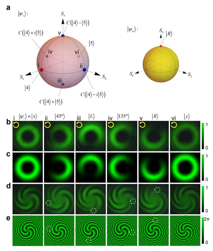
Vol. 27, No. 5 | 4 Mar 2019 | OPTICS EXPRESS 7471

       Fig. 1. Conceptual schematic of three types of spin-orbit converters: Q-plate, J-plate, and
       cascaded J-plates. (a) Q-plates operate on a circular polarization basis (|Ri or |Li) and the
       output OAM states corresponding to these circular polarizations are constrained to hold
       conjugate (equal and opposite) topological charges (|`i and |−`i). (b) J-plates operate on
       arbitrary orthogonal polarization basis ( λ+ or |λ− i) and the two possible output orbital
       states |mi and |ni can be independent. But the output spin states, or polarizations, on which
       these vortex beams are imparted must be the same states as the input spin states with flipped
       handedness (opposite sense of rotation). (c) Cascaded J-plates overcome the restriction
       mentioned above. The output spin states can be another arbitrary orthogonal polarization
       basis ( κ + and |κ − i) independent of the input polarization basis ( λ+ and |λ− i). Here, two
       kets are used in succession to describe spin and orbital states.

the pair; the output polarization state of the beam is determined by the eigen-polarization states
of the last J-plate. This degree of freedom of the cascaded J-plate system can also be used to
produce versatile TAM states and complex structured light.

2.    J-plate design and fabrication
The J-plate is an arbitrary spin-to-orbital angular momentum converter that can transform
two orthogonal input polarizations (denoted by|λ+ i and |λ− i) to a basis of output orthogonal
polarizations with flipped handedness (|(λ+ )∗ i and |(λ− )∗ i) carrying different OAM states, |mi
and |ni, with m and n denoting the imparted OAM quantum numbers. In this work, |mi refers
to the spatial, OAM-carrying phase profile of the beam, i.e., |mi = exp{imφ} where φ is the
azimuthal coordinate on the metasurface. In a general case, we allow the input light to have a
non-zero OAM quantum number, denoted by `. The action of the J-plate can then be written as

                                      J λ+ |`i = (λ+ )∗ |` + mi                                         (1)

and

                                      J |λ− i |`i = |(λ− )∗ i |` + ni .                                 (2)

The eigen-polarization states (or basis, two arbitrary orthogonal polarization states) and their
complex conjugates (with flipped handedness) can be written in a general form: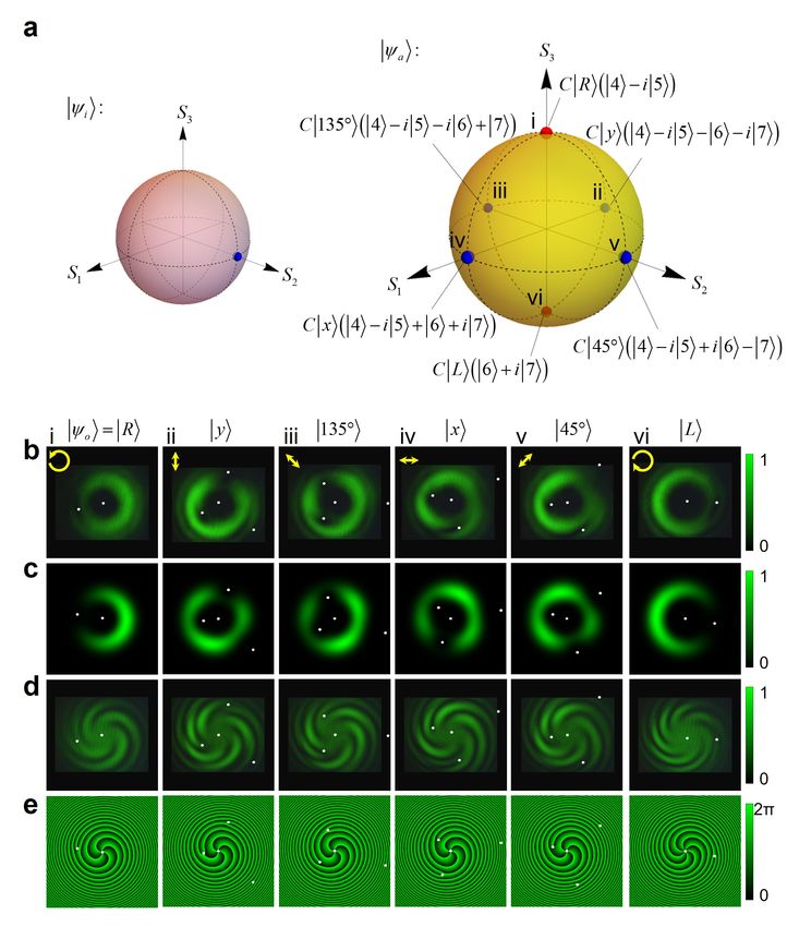
Vol. 27, No. 5 | 4 Mar 2019 | OPTICS EXPRESS 7472
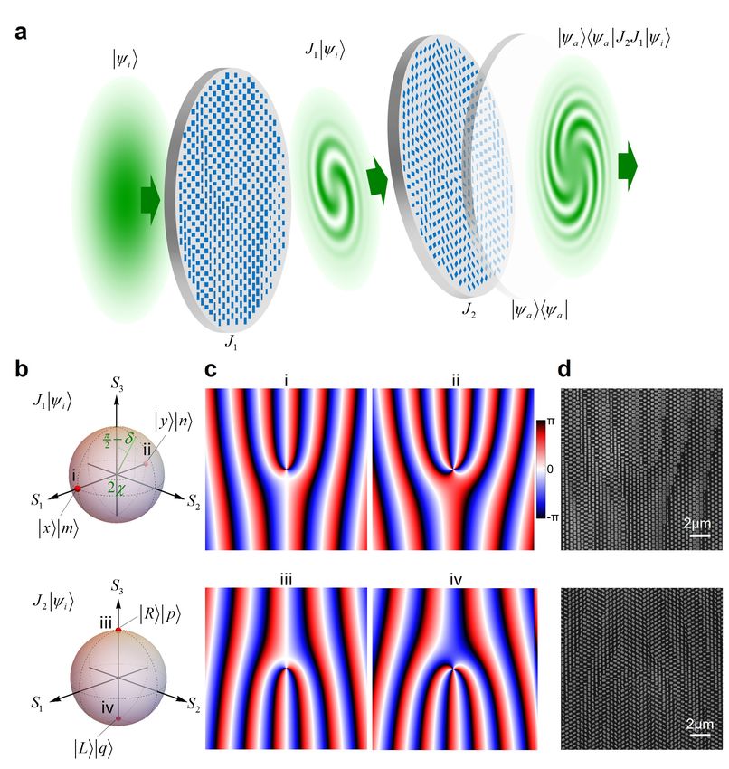
Fig. 2. (a) Schematic: Cascaded J-plates enable the generation of versatile total angular
momentum (TAM) states of light. Bra-ket notation is used for describing how the J-plates
(J1 and J2 ) and analyzer (|Ψ a ihΨ a |) operate on the incident state (|Ψi i). Versatile TAM
states (|Ψ a ihΨ a | J2 J1 |Ψi i) can be generated by selection of incident state, analyzer state,
and the order of J-plates. (b) The higher order Poincaré sphere (HOPS) is a convenient
representation to understand the action of the J-plate on incident light. Two HOPSs represent
the functionality of the J-plates J1 (top) and J2 (bottom). Red dots i-iv mark the eigen-
polarization states and designed TAM states that J1 and J2 can generate: |xi |mi and |yi |ni
for J1 (top) and |Ri |pi and |Li |qi for J2 (bottom). (c) Phase profiles to be imparted on the
eigen-polarization states i-iv of each J-plate. The phase is from two terms, an azimuthal
phase factor of exp(i`φ) and a grating phase along x-axis exp(ik x sin ζ) for tilt output. The
parameters `, and ζ are OAM quantum number and tilt angle of the output beam, respectively.
(d) SEM images of J1 and J2 samples.
cos χ − sin χ cos χ − sin χ
+ + ∗
λ = iδ ; |λ i = iδ
−
; (λ ) = −iδ ; |(λ ) i = −iδ
− ∗
, (3)
e sin χ e cos χ e sin χ e cos χ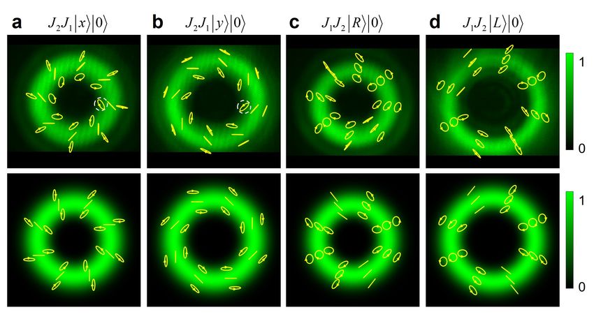
Vol. 27, No. 5 | 4 Mar 2019 | OPTICS EXPRESS 7473

where χ and δ are the orientation angle and double ellipticity angle of a polarization state,
respectively.
   We design two J-plates to work with different polarization bases. The first J-plate (J1 ) is
designed to work in the linear polarization basis, with χ = 0, δ = 0, yielding |xi and |yi as
eigen-polarizations (i.e., simple x- and y-polarized light). The second J-plate (J2 ) is designed to
work in a basis of circular polarization states, with χ = π/4, δ = π/2, yielding |Li and |Ri as
eigen-polarizations. As such, they perform the transformations

                                     J1 |xi |`i = |xi |` + mi ,                                  (4)
                                      J1 |yi |`i = |yi |` + ni ,                                 (5)
                                     J2 |Li |`i = |Ri |` + pi ,                                  (6)
                                     J2 |Ri |`i = |Li |` + qi ,                                  (7)

where parameters m, n, p, and q are designed OAM quantum numbers. To implement the
transformations J1 and J2 , single layer metasurfaces with linear structural birefringence are
used [32]. Figure 2(b) shows the higher-order Poincaré sphere (HOPS) representing all possible
TAM states produced by J1 (top) and J2 (bottom). The three axes S1 , S2 , and S3 correspond to
polarization states |xi, |45◦ i, and |Ri in the positive direction and |yi, |135◦ i, and |Li in the
negative direction. Any polarization state specified by χ and δ can be assigned a position on the
Poincaré sphere with the azimuthal angle (2 χ) and polar angle (π/2 − δ). The red circles mark
the designed eigen-TAM states that each J-plate produces. To satisfy Eqs. (4)-(7), the required
Jones matrix for J1 and J2 as a function of φ are
                                                                imφ
                                                                e     0
                       J1 (φ) = |xihx| e imφ
                                              + |yihy| e inφ
                                                             =              ,                   (8)
                                                                  0  einφ
                                                   1 −(eipφ + eiqφ ) i(eipφ − eiqφ )

           J2 (φ) = |LihR| e ipφ
                                  + |RihL| e iqφ
                                                 =                                      .       (9)
                                                   2 i(eipφ − eiqφ ) (eipφ + eiqφ )
    Ideally, all light incident on J1 or J2 would be directed into the desired OAM mode. However,
in reality, the conversion enacted by metasurface J-plates is not unity, and there is always some
unconverted zeroth order light. While this may be weak for a single metasurface, it can become
significant when several metasurfaces are cascaded, resulting in lower contrast of measured TAM
states. Consequently, we add a grating phase term exp(ik x sin ζ) in the design to separate in
angle the OAM modes of interest from the zeroth order background; the converted light exits at a
tilt angle ζ and undesired light remains in the zeroth order. We set ζ = 10° for J1 and −10° for
J2 , respectively. In this way, the final output beam can propagate along the z-direction and the
non-design term can be blocked during the measurement. In the experiment, we choose m = 2,
n = 3, p = 2, and q = 4. Figure 2(c) shows the required phase profiles of J1 and J2 for the design
polarization as a function of position. Using the method presented in [31, 32], we obtain the
J-plate matrix from the phase profiles (φl and φs ) and orientation angles (θ) as a function of
position.

                                 +                                               −1
                              eiφ (x,y) (λ1+ )∗ eiφ (x,y) (λ1− )∗ (λ1+ ) (λ1− )
                                                    −
                   J(x, y) =     +
                              eiφ (x,y) (λ2+ )∗ eiφ (x,y) (λ2− )∗ (λ2+ ) (λ2− )
                                                     −

                                             iφ (x,y)                                         (10)
                                             e l            0
                           = R[−θ(x, y)]                            R[θ(x, y)]
                                                0      eiφs (x,y)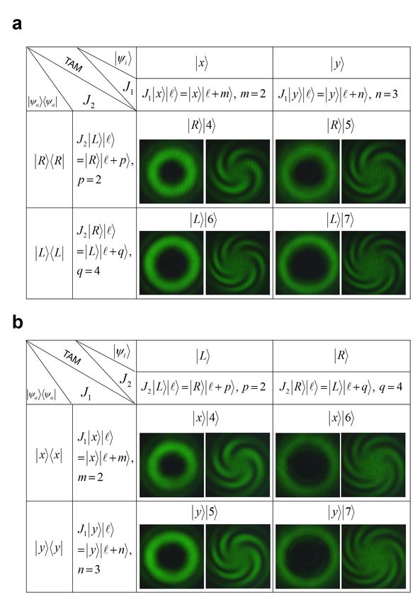
Vol. 27, No. 5 | 4 Mar 2019 | OPTICS EXPRESS 7474

   The J-plates were designed for a wavelength of 532 nm but this design principle can be applied
to any wavelength [32]. The designed J-plates are realized with 600-nm-height TiO2 nanofin
structures on a glass substrate. Different lengths and widths of the structures result in different
phase shifts along the long and short axes (φl and φs ). The TiO2 nanofins are fabricated on fused
silica using electron-beam lithography followed by atomic layer deposition and etching [35].
Figure 2(d) shows scanning electron micrographs (SEMs) of the center sections of J1 (top) and
J2 (bottom). Since J1 operates on a linear basis of polarizations, the phase shift from the nanofins
relies on a propagation phase, resulting in size variation of the rectangular structures without
any rotation (θ = 0). In contrast, the phase shifts from J2 are implemented using a combined
propagation and geometric (Pancharatnam-Berry) phase. J2 consists of several different sizes of
rectangular structures with varying rotation.
   To develop a full understanding of the TAM states that can be generated, we start
from Dirac notation and Jones calculus, where the Jones matrices J1 and J2 are written
in Eqs. (8)-(9). We assume the incident polarization state is a superposition of the two
eigen-polarization states of J1 , |xi and |yi, written as |Ψi i = |αx + βyi, where alpha and
beta are complex numbers chosen such that the incident polarization is normalized. Similarly,
the analyzer state is a superposition of two eigen-polarization state of J2 , |Ri and |Li, writ-
ten as |Ψa ihΨa | = |γR + ηLihγR + ηL|. The state after J2 and before the analyzer can be written as

                   J1 J2 |αx + βyi = |Li hR|xi ei(m+p)φ + |Ri hL|xi ei(m+q)φ
                                                                                               (11)
                                     + |Li hR|yi ei(n+p)φ + |Ri hL|yi ei(n+q)φ .

The output state |Ψo i of J2 J1 after the analyzer can then be written as

          |Ψo i = |Ψa ihΨa | J2 J1 |Ψi i
                = |γR + ηLihγR + ηL| J2 J1 |αx + βyi                                           (12)
                = C[γ(α |m + pi − i β |n + pi) − η(α |m + qi + i β |n + qi)] |γR + ηLi ,

where C is constant that normalizes the final state. Each parameter is in general a complex number.
In our experimental demonstration, m = 2, n = 3, p = 2, and q = 4. Therefore, the output state
|Ψo i can contain four distinct OAM states—|4i, |5i, |6i, and |7i—depending on the incident
polarization and the analyzer, that is, (α, β, γ, η).
   In the field of optical orbital angular momentum and spin-orbit conversion, a so-called higher
order Poincaré sphere (HOPS) is used to visualize superpositions of OAM-carrying beams [36].
In this work, we develop the so-called "cascaded HOPS" that can represent all the output TAM
states as well in an intuitive, visual way. The cascaded HOPS consists of two higher-order
Poincaré spheres depicting the set of possible incident polarizations |Ψi i and the set of possible
analyzer polarizations |Ψa i, respectively. Therefore, a set of two points, one on each sphere,
represents a set of (α, β, γ, η) and consequently an output TAM state.
   By inspection of Eq. (12), it is evident that depending on the values of (α, β, γ, η), the beam
|Ψo i can consist of a superposition of one, two, or four distinct OAM eigen-states. When the
incident polarization is one of the eigen-polarization states of J1 (either α = 0 or β = 0) and the
analyzer state is one of the eigen-polarization states of J2 (either γ = 0 or η = 0), only a single
OAM state emerges (a separable state). In general, however, the output contains two or four OAM
states, a non-separable state (three could occur if n, m, p, and q are chosen such that two of the
four OAM beams carry the same topological charge).
   We examine the separable and non-separable outputs in Sections 3 and 4, respectively.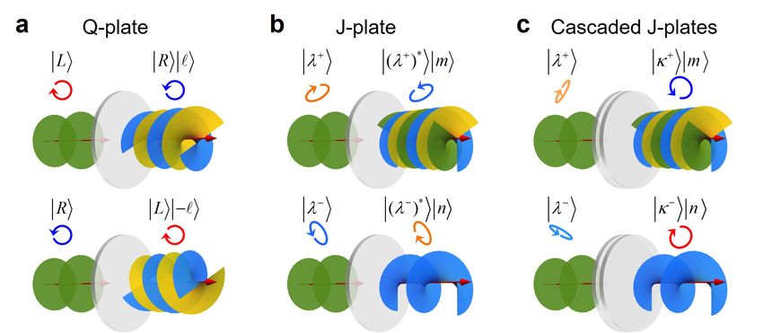
Vol. 27, No. 5 | 4 Mar 2019 | OPTICS EXPRESS 7475

       Fig. 3. (a) These tables document the possible non-separable TAM combinations that can
       be generated by the J-plate cascade, in this case with the light encountering J1 before J2 .
       Measured intensity profiles (left) and interferograms (right) with a reference beam are shown.
       The incident polarization state |Ψi i (|xi or |yi) and final analyzer state |Ψ a ihΨ a | (|RihR| or
       |LihL|) producing the beams are shown at the top and left of the table, respectively. This
       table is a key to determine the output beam with knowledge of the input polarization and
       analyzer configuration. (b) An identical table corresponding to the case where J2 precedes
       J1 , that is, J1 J2 |Ψi i. The corresponding incident states are |Li or |Ri and analyzer states
       are |xihx| or |yihy| in this case.

3.   Single quantum number beams (separable states)
Characterization of the TAM states of a beam requires measurement of both intensity and
phase distribution. The intensity profile of a beam can be measured directly by projecting on a
camera, while the phase profile can be characterized using a Mach-Zehnder interferometer. A
532-nm-wavelength CW laser was used for the measurement. Figure 3 shows, in tabular format,
all possible separable states that the cascaded J-plate pair can generate. Figure 3(a) is for the case
Vol. 27, No. 5 | 4 Mar 2019 | OPTICS EXPRESS 7476 of J2 J1 |Ψi i, where the light passes through J2 after J1 . The images in the table are the measured intensity profiles of TAM states (right) and their corresponding interference patterns (left). The top row of the table records the incident polarization states (|xi or |yi) that form the eigen-basis of the first J-plate J1 . Similarly, the left column of the table records the selection of analyzer polarization states (|RihR| or |LihL|) that are required to isolate a particular separable state. The top and left columns of the table also document the effect of J1 and J2 , respectively. When light with zero OAM passes through the cascaded J-plates, the OAM of the output beam increases to (m + p)~, (m + q)~, (n + p)~, or (n + q)~; all four possibilities are accessible depending on the selection of incident and analyzer polarizations. The measured output states show annular intensity profiles owing to the phase singularity on the beam axis, resulting in the convergence of the spiral fringe pattern. As the OAM quantum number increases, this annular radius increases. The OAM quantum number can be determined by counting the number of arms in the fringe pattern. In this case, the SAM of the separable states is either +~ or −~ because of the circular polarization states. As mentioned above, the J-plates may be exchanged so that light encounters them in the opposite order. Corresponding measurement results in the case of J1 J2 |Ψi i (that is, when light encounters J2 before J1 ) are shown in Fig. 3(b). The generated OAM states are similar to that of the first case (J2 J1 |Ψi i). Four pure OAM quantum numbers are possible (m + p, n + p, m + q, and n + q) with circular incident polarization (either |Li or |Ri) and x-y linear polarization analyzers (either |xihx| or |yihy|, just a linear polarizer). However, the SAM of the output states is zero because of the linear polarization of the analyzer. We note that the cascaded metasurfaces can convert any desired basis of orthogonal polarizations to another, and this output basis is not constrained to be the complex conjugate (flipped handedness version) of the other. As is evident from Fig. 3, both the incident polarization and the configuration of the polarization state analyzer influence the appearance and angular momentum of the output beam. As such, both factors must be considered when conceptualizing the output on the HOPS, which usually only depicts the effect of varying incident polarization with a fixed analyzer configuration. 4. Superposition of TAM states (non-separable states) As shown in Eq. (12), there are an infinite number of ways to generate non-separable states because of the infinite possible configurations of the set (α, β, γ, η). Here, we focus on 3 cases: 1) The input is varied while the final analyzer is fixed at an eigen-polarization state of J2 . 2) The polarization state of the analyzer is varied and the incident polarization is fixed at an eigen-polarization state of J1 . 3) Case 2 with an incident polarization that is not an eigen-polarization of J1 . The cascaded HOPSs that the possible TAM states map onto for these 3 cases are shown in Figs. 4(a), 5(a) and 6(a), respectively. Each consists of two Poincaré spheres that represent the incident polarization state (left, light red sphere) and analyzer state (right, yellow sphere). The output angular momentum states are labeled on the sphere that represents the parameter varied in each figure (either the input or analyzer polarization states). For instance, these are labeled on the incident polarization Poincaré sphere in case 1 (Fig. 4(a)) but labeled on the analyzer Poincaré sphere in case 2 and 3 (Figs. 5(a) and 6(a)). The spin (polarization state) information, however, are labeled on the analyzer Poincaré spheres because the output polarization is always determined by the analyzer. In case 1, we fix the analyzer state as |Ri ((γ, η) = (1, 0), one eigen-polarization state of J2 , the second J-plate), and vary the incident polarization state. The polarization state of this fixed analyzer is shown on the yellow sphere in Fig. 4(a). From Eq. (12) we obtain the output polarization state |Ψo i = C(α |Ri |4i − i β |Ri |5i). Six states (i-vi) are measured and theoretically predicted, as shown in Figs. 4(b)-4(e), while the corresponding Poincaré sphere positions are marked in Fig. 4(a) with small dots. When the incident polarization is one of the eigen-polarization
Vol. 27, No. 5 | 4 Mar 2019 | OPTICS EXPRESS 7477
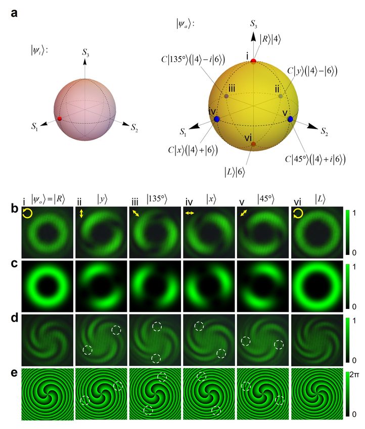
Fig. 4. Beam profiles and interferograms produced when the input is varied and the final
analyzer is kept fixed. If |Ψa i = |Ri, from Eq. (12), |Ψo i = C(α |Ri |4i − i β |Ri |5i) with α
and β parameterizing the input polarization. (a) The cascaded HOPS representing possible
TAM states of J2 J1 while the analyzer state is fixed as |Ri. The cascaded HOPS contains
one sphere for all possible incident polarizations |Ψi i (light red sphere, left) and another one
depicting all possible analyzer polarizations |Ψa i (yellow sphere, right). The dots on the
left HOPS mark the results corresponding to b-e, with red denoting eigenstates and blue
denoting non-eigenstates. (b-e) Measured intensity (b), calculated intensity (c), measured
interferogram (d), and calculated phase profile (e) of the output states. The states in (b-e)
i-vi are marked as dots on the cascaded HOPS in (a). The white dashed circles in (d-e) label
the positions of off-axis singularities in the interferogram and phase profiles.
states of J1 (either |xi or |yi, labeled with red dots), the output state is a separable TAM state,
namely either |Ri |4i or |Ri |5i. When the incident polarization state, however, is an equal
superposition of |xi and |yi with different phases, as is the case when 45° , |Li, 135° , and |Ri
are incident, for instance, a phase shift is introduced between |Ri |4i and |Ri |5i. Figures 4(b)Vol. 27, No. 5 | 4 Mar 2019 | OPTICS EXPRESS 7478
Fig. 5. Beam profiles and interferograms produced when the input is fixed and the final
analyzer is varied. If |Ψi i = |xi, from Eq. (12), |Ψo i = C |γR + ηLi (γ |4i − η |6i) where γ
and η parameterize the analyzer polarization state. (a) The cascaded HOPS representing
possible TAM states of J2 J1 while the incident polarization is fixed as |xi. Here the possible
TAM states are shown on the analyzer sphere. (b-e) Measured intensity (b), calculated
intensity (c), measured interferogram (d), and calculated phase (e) of the output states. The
states in (b-e) i-vi are marked as circles on the cascaded HOPS in (a). The white dashed
circles in (d-e) label the position of the off-axis singularity.
and 4(c) are measured and calculated intensity profiles of these states. Since the states (ii-v) are
equal superposition of two states, we expect |4 − 5| = 1 additional off-axis singularity, resulting
in a null (minimum) in the intensity pattern (Figs. 4(b)(ii-v) and 4(c)(ii-v)) and an off-axis fork in
the interference pattern (white dashed circle in Fig. 4(d)(ii-v)). The positions of calculated nodes,
and phase singularities in Figs. 4(c)(ii-v) and 4(e)(ii-v) match well to the measurement results.
We observe that the rotation angle of this intensity null (Φn ) is the same as the an-Vol. 27, No. 5 | 4 Mar 2019 | OPTICS EXPRESS 7479
Fig. 6. Beam profiles and interferograms produced when the analyzer polarization is varied
and input is fixed at a polarization that is not an eigen-polarization state of J1 . If |Ψi i = |45◦ i,
from Eq. (12), the output state is |Ψo i = C |γR + ηLi (γ |4i − iγ |5i − η |6i − iη |7i) where γ
and η parameterize the polarization state of the analyzer. (a) The cascaded HOPS representing
possible TAM states of J2 J1 while the incident polarization is fixed as |45◦ i. (b-e) Measured
intensity (b), calculated intensity (c), measured interferogram (d), and calculated phase (e)
of the output states. The states in (b-e) i-vi are marked as circles on the cascaded HOPS in
(a). The white dots in (b-e) label the position of off-axis singularities.
gular coordinate (or angular separation shift) on the Poincaré sphere Θ. For instance,
the position shift from incident state (ii) to (iii) on the Poincaré sphere is Θ = 90° . In
turn, the null in the intensity pattern rotates 90° as well. The angular distance Θ canVol. 27, No. 5 | 4 Mar 2019 | OPTICS EXPRESS 7480
be any great-circle distance on the Poincaré sphere. For a superposition of any two OAM
beams with quantum numbers `1 and `2 , the null intensity rotation rate can be written in general as:
∂Φn 1
= . (13)
∂Θ |`1 − `2 |
In the present case with |`1 − `2 | = 1, this is easily understood: The null intensity should rotate 2π
to the same position when the angular distance subtends 2π on the Poincaré sphere. Extending to
any OAM quantum number difference ∆`, the null intensity will rotate 2π/∆` for a change in
angular distance on the Poincaré sphere of 2π. This relation has been demonstrated along the
equator of Poincaré sphere in [33], and is now demonstrated along a line of longitude on the
Poincaré sphere here.
It is also possible to fix the incident polarization while varying the polarization state of the
analyzer. In the cascaded HOPS representation, this would correspond to a fixed point on the
incidence sphere (Fig. 5(a), left) and a varying position on the analyzer sphere (Fig. 5(b), right).
Figure 5 depicts measured results for this case, where the incident polarization state is kept fixed
as |xi ((α, β) = (1, 0), one of the eigen-polarization states of J1 ), and the analyzer polarization
is varied to generate TAM states mapped on the analyzer sphere. Six states (i-vi) are measured
and calculated shown in Figs. 5(b)-5(e), while the mapped positions are marked in Fig. 5a. In
contrast to Fig. 4, the spin (polarization state) and OAM information are labeled together on the
analyzer sphere because they are both determined by the analyzer in this case. When the analyzer
polarization is one of the eigen-polarization states of J2 (either |Ri or |Li, labeled with red dots),
the output state is a separable state given by |Ri |4i or |Li |6i. Changing the angle of the output
linear polarizer (|yi, |135◦ i, |xi, and |45◦ i) introduces a phase shift between |Ri |4i and |Li |6i
in the superposition. This yields two off-axis singularities in the phase profile (Fig. 5(e) (ii-v)),
two off-axis nulls in the intensity pattern (Figs. 5(b) and 5(c)(ii-v)), and two off-axis forks in the
measured interference (Fig. 5(d)(ii-v)). The rotation angle of the null intensity Φn experiences
half of the angular position shift on the Poincaré sphere, in agreement with Eq. (12).
Superpositions of 4 TAM states, the most general case for two cascaded J-plates, are also
demonstrated. Figure 6 shows one of the superposition cases of J2 J1 where the incident
polarization is fixed as |45◦ i and the analyzer polarization is changed. From Eq. (12), the output
state is |Ψo i = C |γR + ηLi (γ |4i − iγ |5i − η |6i − iη |7i). The generated superposition of 4
separable TAM states are mapped on the cascaded HOPS shown in Fig. 6(a). Since the incident
polarization is not one of the eigen-polarization states of J1 , both |xi |2i and |yi |3i are generated
from J1 and are incident on J2 . Neither |xi nor |yi are eigen-polarization states of J2 , resulting in
simultaneous generation of four kinds of non-separable TAM states. If we select either |Ri or |Li
as an analyzer polarization, only superpositions of two separable TAM states can be generated,
which is C[|Ri |4i − i |Ri |5i] or C[|Li |6i + i |Li |7i] respectively. In the most general case
where the analyzer polarization is a superposition of |Ri and |Li (points other than the north and
south poles on the Poincaré sphere), the output state consists of all four possible TAM states.
Figures 6(b)-6(e) show the experimental and calculated results. The white dots label the position
of singularities. The off-axis singularity number equals the difference of smallest and largest
OAM quantum number. This is because, in this case, there are 4 multiples of 2π in phase near
the center but 7 far away from the center. Therefore, three singularities can be observed in the
phase profile (Fig. 6(e)(ii-v)). Notably, there is no rotation symmetry between the states (ii-v) in
Figs. 6(b)-6(e).
5. Vector vortex beams using the cascaded J-plate system
A scalar vortex beam is a beam with OAM having a uniform polarization distribution across
its wavefront. Vector vortex beams, on the other hand, have space-variant polarization in theVol. 27, No. 5 | 4 Mar 2019 | OPTICS EXPRESS 7481
plane transverse to the beam. The cascaded J-plates pair can generate vector vortex beams from
superpositions of separable states. Here we demonstrate 4 kinds of vector vortex beams using the
cascaded J-plate system and investigate their local polarization states.
Figure 7(a) shows the measured (top) and calculated (bottom) intensity patterns and
polarization state diagrams of the superposition of |Ri |4i and |Li |6i. In principle, different
polarization states are unable to interfere unless projected to a same polarization state using an
analyzer. If there is no analyzer, directly superposing TAM states |Ri |4i and |Li |6i results in
a sum of the two annular intensity profiles, an wider annular intensity profile, shown in Fig.
7(a). Because the annular intensity profiles of |Ri |4i and |Li |6i are different, we expect the
polarization state to change with radius. We can analyze any local polarization state by projecting
it onto 6 polarization states |xi, |yi, |45◦ i, |135◦ i, |Ri, and |Li (Fig. 5(b)). The Stokes vector at
® y) can be calculated from the 6 measured, spatially-varying power images
each position S(x,
®
P(x, y) [32]:
Px 1 1 0 0
Py 1 −1 0 0 S0
P45 1 0 1 0 S1
P® = = = AS,
® (14)
P135 1 0 −1 0
S2
P L 1 0 0 1 S3
PR 1 0
0 −1
S® = (AT A)−1 AT P® (15)
This over-determined linear system is meant to convey that the Stokes vector at each point is
projected onto six different analyzer Stokes vectors (the rows of A) in a way that can be inverted
in the least-squares sense. The vector as a function of position P(x, ® y) can be measured using a
camera with appropriate polarization optics placed in front. The yellow arrows in Fig. 7(a) show
the local polarization ellipse of |Ri |4i + |Li |6i, which is the result of sending |xi polarized light
onto the cascade of J1 followed by J2 , notably with no analyzer. The state can be understood
from Eq. (11). RCP and LCP respectively dominate the sense of rotation of the polarization states
at the inner and outer radius of the annular pattern, as expected. In the middle, RCP and LCP
components contribute equal intensity, resulting in linear polarization.
Figure 7(b) shows the results of superposing of |Ri |5i and |Li |7i (the result of sending |yi
polarized light onto the cascade of J1 followed by J2 , notably with no analyzer), where RCP and
LCP respectively dominate the inner and outer radius of the annular pattern as well. However, the
polarization diagram of each labeled position is quite different from Fig. 7(a). This is evident by
comparing the polarization ellipses in the white dashed circles labeled in Figs. 7(a) and 7(b). In
Fig. 7(a), the elliptical polarization shows an obvious combination of 135° and |Ri while in Fig.
7(b), it shows a combination of 45° and |Ri. This is a result of the different phases between the
superpositions of the two states, as can be seen from the Dirac notation of the state written in Eq.
(11). In Fig. 7(a), where the output state is J2 J1 |xi |0i, the phase between terms hR|xi and hL|xi
is π. In Fig. 7(b), where the state generated is J2 J1 |yi |0i, the phase between terms hR|yi and
hL|yi is 0.
Figures 7(c) and 7(d) show the superposition of |xi |4i and |yi |5i (the result of sending |Ri
polarized light onto the cascade of J2 followed by J1 , notably with no analyzer) and |xi |6i and
|yi |7i (the result of sending |Li polarized light onto the cascade of J2 followed by J1 , notably
with no analyzer). Linear polarization is observed at the upper left and lower right corner. RCP
dominates at the upper right in Fig. 7(c) and lower right in Fig. 7(d) while LCP dominates at the
opposite position. We note that it is possible to generate more complex vector vortex beams from
superposition of 4 separable states, such as J2 J1 |Ri |0i, J1 J2 |xi |0i, etc.Vol. 27, No. 5 | 4 Mar 2019 | OPTICS EXPRESS 7482
Fig. 7. The measured (top row) and calculated (bottom row) intensity profile of 4 TAM states
and the polarization ellipse diagrams. (a) Superposition of |Ri |4i and |Li |6i produced by
J2 J1 |xi |0i. (b) Superposition of |Ri |5i and |Li |7i produced by J2 J1 |yi |0i. (c) Superpo-
sition of |xi |4i and |yi |5i produced by J1 J2 |Li |0i. (d) Superposition of |xi |6i and |yi |7i
produced by J1 J2 |Ri |0i.
6. Conclusion
In this work, we introduced and demonstrated the notion of cascaded J-plates. Notably, the output
polarization states of these J-plates are not constrained to the complex conjugate of the input
polarization state, in contrast to previous work. With these cascaded J-plates, we demonstrate
versatile generation of TAM modes, including separable and non-separable TAM modes. We
also introduced the notion of the cascaded higher-order Poincaré sphere, which we use to map
our results. In all, the system of two cascaded J-plates can generate eight distinct separable states,
eight distinct superposition states of two separable states, eight distinct superpositions of four
separable states, and four varieties of vector vortex beams. In principle, the system can generate
an infinite number of non-separable states if we consider the cases of unequal superposition.
There is of course the possibility to cascade more than two J-plates. While a simple cascade of
two has been demonstrated here, the analytic methods we present can of course extend to more
than two cascaded metasurfaces. A single layer metasurface can be designed for generating any
one kind of TAM states or vector vortex beams. Cascaded metasurfaces offer more degrees of
freedom, namely variable incident polarization, variable analyzer polarization, and switching
the order of the metasurfaces, etc, to select or generate more possible TAM states, vector vortex
beams, and complex structured light.
Funding
Air Force Office of Scientific Research (MURI FA9550-14-1-0389, FA9550-16-1-0156); King
Abdullah University of Science and Technology (KAUST) Office of Sponsored Research (OSR)
(OSR-2016-CRG5-2995); National Research Foundation, Prime Minister’s Office, Singapore
(NRF-CRP15-2015-03); National Science Foundation (1541959, DGE1144152).
Acknowledgments
This work was supported in part by the Air Force Office of Scientific Research (Grant Nos.
MURI FA9550-14-1-0389 and FA9550-16-1-0156) and King Abdullah University of ScienceVol. 27, No. 5 | 4 Mar 2019 | OPTICS EXPRESS 7483
and Technology (KAUST) Office of Sponsored Research (OSR) (Award No. OSR-2016-CRG5-
2995). C.W.Q. and Y.W.H. acknowledge support from the National Research Foundation, Prime
Minister’s Office, Singapore under its Competitive Research (CRP Award No. NRF-CRP15-2015-
03). N.A.R. acknowledges support from the National Science Foundation Graduate Research
Fellowship Program under grant no. DGE1144152. This work was performed in part at the
Center for Nanoscale Systems (CNS), a member of the National Nanotechnology Coordinated
Infrastructure (NNCI), which is supported by the National Science Foundation under NSF award
no. 1541959. CNS is a part of Harvard University.
Disclosures
The authors declare that there are no conflicts of interest related to this article.
References
1. J. H. Poynting, “The wave motion of a revolving shaft, and a suggestion as to the angular momentum in a beam of
circularly polarised light,” Proc. R. Soc. Lond., A Contain. Pap. Math. Phys. Character 82, 560–567 (1909).
2. R. A. Beth, “Mechanical detection and measurement of the angular momentum of light,” Phys. Rev. 50, 115 (1936).
3. H. Kogelnik and T. Li, “Laser beams and resonators,” Appl. Opt. 5, 1550–1567 (1966).
4. C. Tamm, “Frequency locking of two transverse optical modes of a laser,” Phys. Rev. A 38, 5960 (1988).
5. P. Coullet, L. Gil, and F. Rocca, “Optical vortices,” Opt. Commun. 73, 403–408 (1989).
6. L. Allen, M. W. Beijersbergen, R. J. C. Spreeuw, and J. P. Woerdman, “Orbital angular-momentum of light and the
transformation of laguerre-gaussian laser modes,” Phys. Rev. A 45, 8185–8189 (1992).
7. S. Van Enk and G. Nienhuis, “Commutation rules and eigenvalues of spin and orbital angular momentum of radiation
fields,” J. Mod. Opt. 41, 963–977 (1994).
8. A. Kumar, P. Vaity, and R. P. Singh, “Crafting the core asymmetry to lift the degeneracy of optical vortices,” Opt.
Express 19, 6182–6190 (2011).
9. M. Beijersbergen, R. Coerwinkel, M. Kristensen, and J. Woerdman, “Helical-wavefront laser beams produced with a
spiral phaseplate,” Opt. Commun. 112, 321–327 (1994).
10. E. Karimi, S. A. Schulz, I. De Leon, H. Qassim, J. Upham, and R. W. Boyd, “Generating optical orbital angular
momentum at visible wavelengths using a plasmonic metasurface,” Light. Sci. & Appl. 3, e167 (2014).
11. N. Shitrit, I. Bretner, Y. Gorodetski, V. Kleiner, and E. Hasman, “Optical spin hall effects in plasmonic chains,” Nano
Lett. 11, 2038–2042 (2011).
12. G. Spektor, D. Kilbane, A. Mahro, B. Frank, S. Ristok, L. Gal, P. Kahl, D. Podbiel, S. Mathias, H. Giessen, F.-J.
Meyer zu Heringdorf, M. Orenstein, and M. Aeschlimann, “Revealing the subfemtosecond dynamics of orbital
angular momentum in nanoplasmonic vortices,” Science. 355, 1187–1191 (2017).
13. M. Padgett and R. Bowman, “Tweezers with a twist,” Nat. Photonics 5, 343 (2011).
14. G. Gibson, J. Courtial, M. J. Padgett, M. Vasnetsov, V. Pasko, S. M. Barnett, and S. Franke-Arnold, “Free-space
information transfer using light beams carrying orbital angular momentum,” Opt. Express 12, 5448–5456 (2004).
15. J. Wang, J.-Y. Yang, I. M. Fazal, N. Ahmed, Y. Yan, H. Huang, Y. Ren, Y. Yue, S. Dolinar, M. Tur, S. Dolinar, M. Tur,
and A. E. Willner, “Terabit free-space data transmission employing orbital angular momentum multiplexing,” Nat.
Photonics 6, 488 (2012).
16. H. Ren, X. Li, Q. Zhang, and M. Gu, “On-chip noninterference angular momentum multiplexing of broadband light,”
Science 352, 805–809 (2016).
17. E. Nagali, F. Sciarrino, F. De Martini, L. Marrucci, B. Piccirillo, E. Karimi, and E. Santamato, “Quantum information
transfer from spin to orbital angular momentum of photons,” Phys. Rev. Lett. 103, 013601 (2009).
18. R. Fickler, R. Lapkiewicz, W. N. Plick, M. Krenn, C. Schaeff, S. Ramelow, and A. Zeilinger, “Quantum entanglement
of high angular momenta,” Science. 338, 640–643 (2012).
19. K. Huang, H. Liu, S. Restuccia, M. Q. Mehmood, S.-T. Mei, D. Giovannini, A. Danner, M. J. Padgett, J.-H. Teng, and
C.-W. Qiu, “Spiniform phase-encoded metagratings entangling arbitrary rational-order orbital angular momentum,”
Light. Sci. & Appl. 7, 17156 (2018).
20. S. W. Hell and J. Wichmann, “Breaking the diffraction resolution limit by stimulated emission: stimulated-emission-
depletion fluorescence microscopy,” Opt. Lett. 19, 780–782 (1994).
21. A. Nicolas, L. Veissier, L. Giner, E. Giacobino, D. Maxein, and J. Laurat, “A quantum memory for orbital angular
momentum photonic qubits,” Nat. Photonics 8, 234 (2014).
22. D. Naidoo, F. S. Roux, A. Dudley, I. Litvin, B. Piccirillo, L. Marrucci, and A. Forbes, “Controlled generation of
higher-order poincaré sphere beams from a laser,” Nat. Photonics 10, 327–332 (2016).
23. P. Miao, Z. Zhang, J. Sun, W. Walasik, S. Longhi, N. M. Litchinitser, and L. Feng, “Orbital angular momentum
microlaser,” Science 353, 464–467 (2016).
24. M. Babiker, C. Bennett, D. Andrews, and L. D. Romero, “Orbital angular momentum exchange in the interaction of
twisted light with molecules,” Phys. Rev. Lett. 89, 143601 (2002).Vol. 27, No. 5 | 4 Mar 2019 | OPTICS EXPRESS 7484
25. G. Biener, A. Niv, V. Kleiner, and E. Hasman, “Formation of helical beams by use of pancharatnam-berry phase
optical elements,” Opt. Lett. 27, 1875–1877 (2002).
26. L. Marrucci, C. Manzo, and D. Paparo, “Optical spin-to-orbital angular momentum conversion in inhomogeneous
anisotropic media,” Phys. Rev. Lett. 96, 163905 (2006).
27. M. Khorasaninejad and F. Capasso, “Metalenses: Versatile multifunctional photonic components,” Science. 358,
eaam8100 (2017).
28. R. C. Devlin, A. Ambrosio, D. Wintz, S. L. Oscurato, A. Y. Zhu, M. Khorasaninejad, J. Oh, P. Maddalena, and
F. Capasso, “Spin-to-orbital angular momentum conversion in dielectric metasurfaces,” Opt. Express 25, 377–393
(2017).
29. Z. J. Shi, M. Khorasaninejad, Y. W. Huang, C. Roques-Carmes, A. Y. Zhu, W. T. Chen, V. Sanjeev, Z. W. Ding,
M. Tamagnone, K. Chaudhary, R. C. Devlin, C. W. Qiu, and F. Capasso, “Single-layer metasurface with controllable
multiwavelength functions,” Nano Lett. 18, 2420–2427 (2018).
30. A. Arbabi, Y. Horie, M. Bagheri, and A. Faraon, “Dielectric metasurfaces for complete control of phase and
polarization with subwavelength spatial resolution and high transmission,” Nat. Nanotechnol. 10, 937 (2015).
31. J. P. B. Mueller, N. A. Rubin, R. C. Devlin, B. Groever, and F. Capasso, “Metasurface polarization optics: Independent
phase control of arbitrary orthogonal states of polarization,” Phys. Rev. Lett. 118, 113901 (2017).
32. R. C. Devlin, A. Ambrosio, N. A. Rubin, J. P. B. Mueller, and F. Capasso, “Arbitrary spin-to-orbital angular
momentum conversion of light,” Science. 358, 896–900 (2017).
33. E. J. Galvez, S. Khadka, W. H. Schubert, and S. Nomoto, “Poincare-beam patterns produced by nonseparable
superpositions of laguerre-gauss and polarization modes of light,” Appl. Opt. 51, 2925–2934 (2012).
34. Y. Li, X. Li, L. Chen, M. Pu, J. Jin, M. Hong, and X. Luo, “Orbital angular momentum multiplexing and demultiplexing
by a single metasurface,” Adv. Opt. Mater. 5, 1600502 (2017).
35. R. C. Devlin, M. Khorasaninejad, W. T. Chen, J. Oh, and F. Capasso, “Broadband high-efficiency dielectric
metasurfaces for the visible spectrum,” Proc. Natl. Acad. Sci. United States Am. 113, 10473–10478 (2016).
36. G. Milione, H. Sztul, D. Nolan, and R. Alfano, “Higher-order poincaré sphere, stokes parameters, and the angular
momentum of light,” Phys. Rev. Lett. 107, 053601 (2011).You can also read