Efficient Resampling, Compression and Rendering of Metallic and Pearlescent Paint
←
→
Page content transcription
If your browser does not render page correctly, please read the page content below
Efficient Resampling, Compression and Rendering of Metallic and
Pearlescent Paint
Martin Rump, Ralf Sarlette, Reinhard Klein
Institute for Computer Science II, University of Bonn
Email: {rump, sarlette, rk}@cs.uni-bonn.de
Abstract been proposed for this kind of material. While
model based representations (like [1]) are quite
An interesting class of materials are metallic and powerful, they cannot represent all of the complex
pearlescent paints. They pose serious challenges effects inside of metallic and pearlescent paints.
to computer graphics since they have high frequen- This is especially true for the spatial variations.
cies in both angular and spatial domain, have a Purely image based approaches avoid these prob-
complex, pure stochastic spatial structure and an- lems but simultaneously introduce others. The
gular dependent color shifts. Hybrid approaches amount of data is critical since the sampling in an-
that combine model and image-based representa- gular domain must be very high to capture the ef-
tions have proven to faithfully reproduce metal- fects around the highlight direction and the high an-
lic and pearlescent paint by compressing measured gular frequecies of the glittering effects.
data. But until now the compression of the image
Hybrid approaches combining model and image
based part is done with PCA based methods result-
based methods can circumvent many of these prob-
ing in high amounts of data. One additional prob-
lems and faithfully reproduce metallic and pearles-
lem is the angular sampling of the measured data.
cent paints. Rump et al. [5] started with an image
Typical angular sampling densities of image based
based representation by measuring real paint sam-
reflectance acquisition devices are very low com-
ples and split the data into a homogeneous (spatially
pared to the solid angle, in which a metallic flake is
invariant) part and a spatially varying part that is
visible, resulting in severe undersampling of the an-
kept as a BTF capturing primarily the appearance
gular frequencies. We propose a simple method to
of flakes (see Figure 1). However, the method has
measure these frequencies generated by the metallic
two main drawbacks.
flakes. Furthermore, we present a novel representa-
tion for metallic and pearlescent paint that allows First, the compression of the image based part us-
resampling in angular domain corresponding to the ing PCA lacks efficiency and introduces artefacts,
flake properties and compression of measured im- especially blurred flakes (see Figure 6). They had
age based paint data for high-quality paint render- to choose a high number of components to pre-
ing. serve the appearance of the flakes resulting in high
amounts of data and slow decoding speed. The
1 Introduction stochastic nature of the spatial and angular varia-
Photo-realistic rendering of car paint is of great in- tions of metallic paints is a general problem since
terest for the automotive industry since lacquered compression methods suitable for rendering assume
surfaces contribute most to the overall visual ap- similarities or regular behaviour on a per-texel ba-
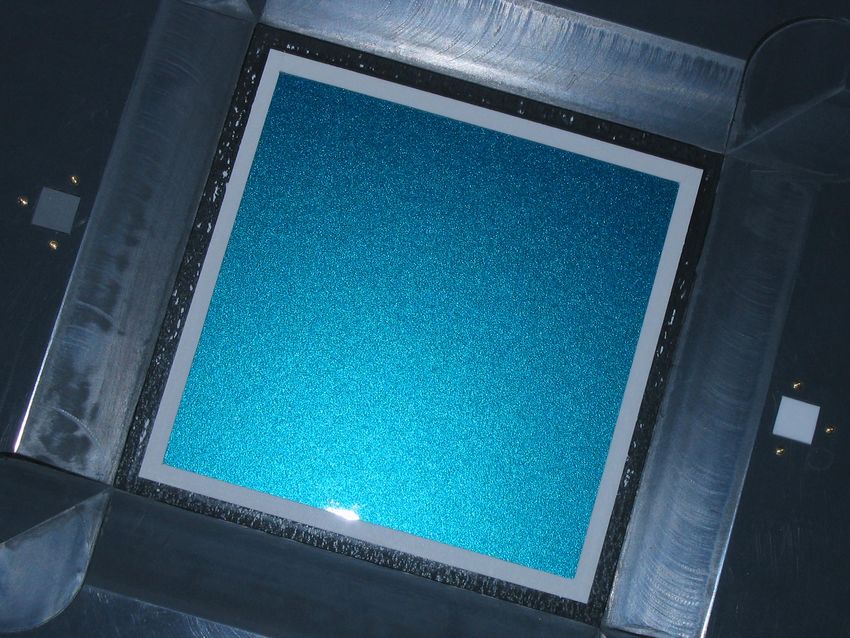
pearance of their products. But also other products sis. Figure 2 shows two images of metallic car paint
like mobile phones or digital cameras are lacquered with slightly varied light direction. It can be noticed
with metallic or pearlescent paints to improve their that the positions of the sparkling effects change
look. For rendering purposes these paints need an completely. Second, the angular sampling of the
elaborate representation since they show a high- BTF measurement is by far not sufficient to repro-
dynamic-range in intensities, complex spatial varia- duce the angular frequencies of the flake glittering.
tions, high angular frequencies due to glittering and In this paper we present a simple method to measure
angular dependent color effects. the angular sampling density that would be neces-
By now, model and image based methods have sary to reproduce the glittering of the flakes of a cer-
VMV 2009 M. Magnor, B. Rosenhahn, H. Theisel (Editors)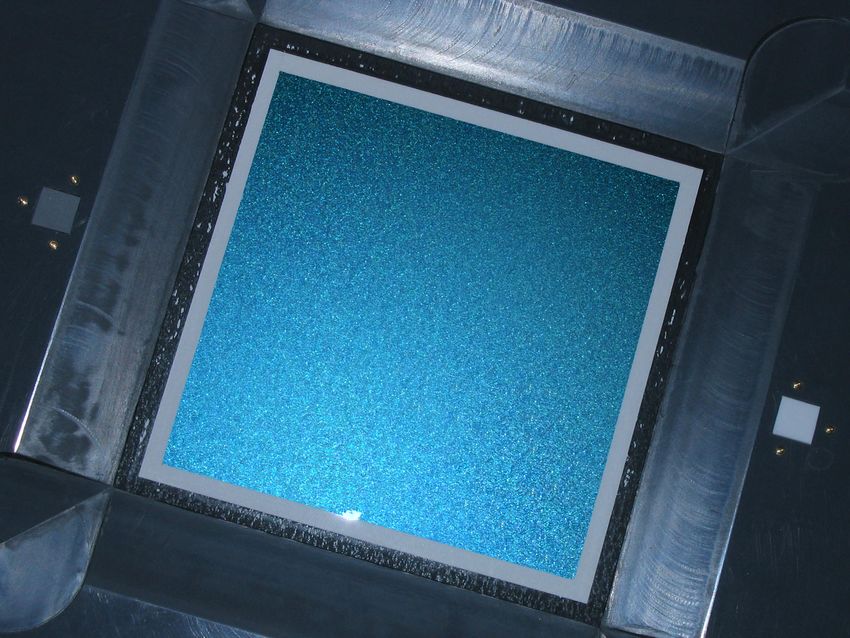
Figure 2: The same excerpt of a metallic paint
                                                          measurement with a slightly varying light direction
Figure 1: Typical metallic flake BTF image, gen-          (11◦ ). Please note that the positions of the sparkles
erated by subtracting the homogeneous part from           change completely from one image to the other.
the original measured data. This image corresponds
to about 7x7cm of paint. The angular variations of        mals to achieve consistent flake glittering in anima-
roughly 7◦ causes significantly varying sparkle den-      tions of lacquered surfaces.
sity.                                                        Unfortunately, the effects in metallic paints are
                                                          very complex and thus even the detailed model of
tain paint correctly. Typically, necessary sampling       Ershov does not reproduce the spatial variations of
distances for metallic paint are under 3◦ whereas         such paints totally. Additionally, the sparkling ef-
many BTF measurement devices only provide sam-            fects in pearlescent paints are even more complex,
plings of 15◦ or even sparser resulting in wrong im-      since the flakes have thin coatings leading to color
pressions of the glittering effect if the measured data   shifts dependent on illumination and viewing angle
is rendered in a naive way. We present a method that      and thus to colored sparkling. In contrast to this, im-
exploits angular variations present in BTF datasets       age based methods like BTF can reproduce all the
and which is able to resample the image data in an-       complex spatial effects of metallic and pearlescent
gular domain to match the necessary angular resolu-       paint.
tion. Our method supports compression of the large
amounts of data with a better ratio than PCA us-          2.2   BTF compression
ing an example based approach. Since the examples
                                                          A bidirectional texture function (BTF) is a six di-
are stored without further compression, our method
                                                          mensional function ρ(x, ωi , ωo ) with x as spatial
does not suffer from blurred flakes.
                                                          position and ωi , ωo as light and view direction. BTF
   The paper is organized as follows: Section 2
                                                          data of metallic paints has nearly no correlation in
summarizes previous work on the topics car paint
                                                          all six dimensions. Both the spatial as well as the
modelling and BTF compression. Section 3 gives
                                                          angular variations cover a broad frequency band in-
an overview about our proposed model and algo-
                                                          cluding very sharp peaks.
rithms that are then explained in more detail in the
                                                             Most of previous BTF compression techniques
following sections. The paper is concluded with re-
                                                          rely on matrix or tensor factorization (e.g. [6], [7])
sults in Section 6 and 7.
                                                          sometimes combined with clustering (e.g. [4]) or
                                                          the fitting of analytical models to the texels of the
2     Previous Work
                                                          BTF (e.g. [3]). Since all these methods exploit ei-
2.1    Paint models                                       ther correlations in some dimensions of the dataset
Ershov et al. [1] proposed a physically based model       or regular behaviour on a per-pixel basis they can-
for the sparkling effects of metallic paints. They as-    not be applied here.
sumed that the metallic flakes are mirror like and           Rump et al. [5] used a PCA based method to
have a gaussian size and orientation distribution.        compress the image based data. Therefore, they
They showed how to efficiently decide if a pixel          did not achieve good compression ratios and had to
on a lacquered surface contains a sparkling effect        keep only a small slice of the BTF. Nevertheless,
or not, and what the reflected energy from the ran-       they observed that small rectangular patches of a
domly generated flake is. Günther et al. [2] ex-         metallic paint BTF image are quite different when
tended this approach using a texture of flake nor-        compared on a per-pixel basis, but they have similar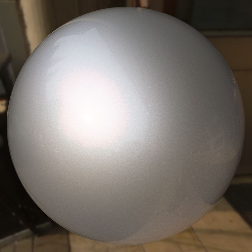
Paint sample
statistical properties like mean intensity or sparkle
density. Exploring this observation they proposed
a simple patch based synthesis by copying these
patches randomly beneath each other.
3 Overview Lamp
We follow the general approach of Rump et al. [5] Camera
and decompose the measured data into a homoge-
neous part and a spatially varying, image based part Figure 3: Setup for the measurement of glittering
represented by a BTF. frequency.
In contrast, we do not use this BTF part in a sim-
ple way but introduce a novel method to resample In the captured video the flakes smoothly fade in
and compress this part. To obtain the correct angu- and out (see multimedia material). The basic idea
lar sampling rate for the BTF we measure the angu- is to measure the number of video frames ∆tf lakes
lar frequency of the glittering from the flakes. This the flakes are visible. The corresponding duration in
is explained in Section 4. relation to the rotation speed ωrot of the lamp pro-
Our resampling exploits the fact, that the view- vides the angular spread βf lakes of the light scatter-
ing and lighting distances of our BTF measurement ing at the flakes and thus the angular frequency of
setup are quite small. This leads to significant an- the glittering effects. To get stable results we used a
gular variation across the sample which can be seen video camera with 15 FPS and turned the lamp with
in Figure 1. Due to this angular variations the mea- the speed of 1◦ /second over an angular range of 90◦
surement setup provides data for a much greater set ending up with 1350 video frames.
of directions compared to its native angular reso- Since the camera is fixed with respect to the paint
lution and thus enough information to resample the sample, the flakes stay at constant pixel positions.
BTF part to a higher angular resolution that matches The energy value corresponding to a certain pixel
the glittering effects well. Our method supports re- over time shows essentially a combination of two
sampling and compression at a time by first choos- effects: light scattering due to the basis BRDF of
ing a desired angular sampling and then selecting the paint and scattering due to the roughness of in-
a set of small representative data slices for every dividual flakes in the footprint of the pixel on the
direction and synthesizing from these slices during paint. Both scattering processes can be modelled
decompression. Details for resampling and com- using a gaussian lobe. Since the optics of the cam-
pression can be taken from Section 5. era causes a gaussian shaped blurring in spatial do-
main we fit a three dimensional gaussian mixture
4 Flake property measurement model to the pixel intensity functions over time
F (x, y, t) minimizing the following error function:
Since the BTF measurement suffers from angular v
undersampling it does not provide enough informa- u
uX X T
(F (x, y, t) − M (x, y, t, µ, σ, S))2 (1)
u
E(µ, σ, S) = t
tion about the angular frequency of glittering effects x,y t=1
caused by the metallic flakes in the paint. Therefore
M (x, y, t, µ, σ, S) =
we propose a simple method to measure this fre- NG
X
(x − µ1,i )2 (y − µ2,i )2 (t − µ3,i )2
quency that is directly connected to the BRDF of Si exp −
2σ 2
−
2σ 2
−
2σ 2
i=1 1,2,i 1,2,i 3,i
the single flakes. We assume that the flakes them- (2)
selves have isotropic reflectance. Anisotropy of the The number of gaussian lobes NG must be vari-
flakes would be quite difficult to measure since they able in the optimization process to adapt to different
are rotated arbitrarily inside the paint and for good flake densities. The variances σ1 and σ2 are com-
results a statistic over a large amount of flakes is bined to one variance σ1,2 assuming isotropic flakes
needed. Figure 3 shows our simple setup that con- in spatial domain. This reduces the dimensionality
sists of a video camera facing the paint sample as of the error function.
well as a lamp emiting directional light, that can be To extract ∆tf lakes from the GMM we build a
moved on a half circle around the sample with con- histogram over all σ3,i for which the scale Si >
stant speed. Sthresh . Sthresh is normally choosen to be about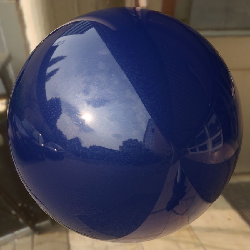
70
Data
Model
main is used to reproduce the measured angular fre-
60
G1
G2
quencies of the paint.
50
G3
Our method exploits the angular variations across
Pixel Value [ ]
G4
40
G5
G6
the measured paint sample due to the finite view-
30
G7
ing and lighting distances during measurement (see
20
Figure 1). We assume that the statistical proper-
10
ties like the sparkle distribution are constant over
0
200 400 600 800 1000 1200
Time [frames] small patches of size between 1.5mm and 3mm of
Figure 4: Intensity of a pixels of the video stream the flake BTF and depend only on light and view
over time and the fitted gaussian mixture model direction. In our experiments we found that patches
showing two significant flakes for this pixel. of size smaller than 1.5mm do not represent all im-
portant statistical properties.
300
A naive approach would be to represent the flake
250 silver metallic paint
blue-green pearlescent paint
BTF as a large set of these small patches with their
200
dark blue metallic paint
respective pairs of view and light direction. For
Counts
150
a dataset with 512x512 pixels, 100x100 view and
100
light directions and a patch size of 16x16 pixels we
50
end up with 32x32x100x100 ≈ 10 million individ-
0
0 10 20
16.25 17.00 17.75
30 40
σ3 50 60 70 80 ual patches leading to impractical amounts of data.
Figure 5: σ3 -histogram of the gaussian mixture The basic idea of our algorithm is to select a sub-
model fitted to the flake video stream of three paints set P of all patches Pall that still represents the
with different flake densities and roughnesses. The whole flake BTF faithfully. As a final representa-
maximum value marks the primary angular fre- tion we only keep this subset of patches and a bidi-
quency of the flake glittering. rectional and spatial look-up table λ(x, ωi , ωo ) that
defines which patch is to be used dependent on po-
sition x and view/light direction ωo , ωi during de-
20% of the maximum pixel value, filtering out compression of the BTF. The decompression step is
smaller bumps in the pixel energies over time. This very efficient since it consists only of one lookup in
is reasonable since we only want to measure the an- the table to select the corresponding patch in P and
gular spread of the flake glittering and not a total then a pixel lookup in the patch itself:
number of flakes. All visual information is still kept ρBT F (x, ωi , ωo ) = Pλ(x̂,ωi ,ωo ) (x − x̂) (5)
in the BTF and thus no information is lost by filter-
ing the σ3,i . After building the histogram we extract having x̂i = bxi /patchsizec. To come up with
the maximum value from it ending up with the cor- a smooth fading of the flakes we perform a simple
responding σf lakes . We then take the width of a linear interpolation in angular domain between the
gaussian distribution with σ = σf lakes at a height discrete ωi , ωo during decompression as it is usually
of 5% to determine ∆tf lakes and βf lakes : performed in BTF rendering.
p The images in P are stored without further
∆tf lakes = 2σf lakes −2ln(0.05) (3) compression preserving the full sharpness of the
∆tf lakes sparkling effects. Of course, a lossless compression
βf lakes = ωrot (4) may still be used to store the images onto the hard
FPS
drive, but for fast lookup during decompression it is
Figure 5 shows the histograms for three differ- inevitable to have the patches unpacked in memory.
ent paints including the σf lakes corresponding to A first idea to find the subset P would be to clus-
βf lakes between 5.3◦ and 5.8◦ . ter Pall by using a pixel-wise distance measure. As
explained in Sections 1 and 2 this is not feasible for
flake BTFs since the patches might be very differ-
5 Resampling and Compression
ent on a per-pixel basis but represent similar parts
In this section we describe our resampling and com- of the metallic paint.
pression method for the spatially varying BTF part The second idea to come up with a patchset P
ρBT F of the paint. The resampling in angular do- would be to cluster the patches with respect to their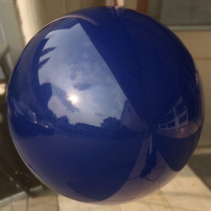
statistical properties. We found out that an intensity responding to each direction pair dcenter ∈
histogram per color channel is sufficient to describe ΩV × ΩL .
this statistical properties. A normalized histogram 3. Select a representative set of patches for each
can be understood as a probability distribution on dcenter
the pixel intensities, and thus it contains all infor- Afterwards, the look-up table λ(x̂, ωi , ωo ) is built
mation about the probability of sparkling effects of with indices into the set P .
a certain energy inside a patch. Unfortunately, stan-
dard clustering does not work here, since the dis- Feature space Using histograms in a standard
tribution of the histograms of Pall is quite non uni- way leads to two practical problems. On the one
form. While the majority of patches is quite dark hand, many pixel intensities of flake BTFs are close
lying in off-specular directions, only a small frac- to zero since the homogeneous part has been sub-
tion located around the highlight direction contains tracted from them. Nevertheless, resolving differ-
the visual important information. Therefore, stan- ences in this intensity region is very important since
dard clustering algorithms tend to place most clus- otherwise seams between the patches could easily
ter centers in the oversampled regions of the space be detected by the human visual system. Therefore,
and thus in the dark regions of the paint. This way very small bins must be choosen what drastically in-
the visual important information is lost. creases the histogram size and therefore decreases
the evaluation speed of distance functions on the
Therefore, instead of applying a standard cluster-
histograms. On the other hand, histograms suffer
ing algorithm, we preselect a discrete set of view
from the discrete nature of the bins. Two sparkle
and light directions ΩV , ΩL and calculate a his-
effects with slightly different intensities may yield
togram for every pair that represents the visual char-
very different histograms. Of course, distance mea-
acteristics of the flake BTF for the respective view
sures like the Earth Movers Distance circumvent the
and light directions. Finally, a small set of represen-
problem but in our setting they are too expensive to
tative patches is assigned to every pair by selecting
compute.
the best fitting patches comparing the histograms of
Therefore, to deal with the value concentration
the direction pair and the patches. This way we can
near zero we use unevenly spaced bins to increase
guarantee to preserve the visual important informa-
sampling density in that region. To avoid the prob-
tion present in the original dataset and to keep the
lems with discrete histogram bins we use gaussian
flake statistics of the measured data. The compres-
filters on the pixel intensity to blur the histogram
sion ratio is determined by the size of ΩV × ΩL
bins. The following formula defines the centers and
and the number K of assigned patches per direction
variances of the unevenly spaced filters:
pair.
Since ΩV , ΩL can be freely specified and since i + 0.5
!γ
µi = τ + (1 − τ ) µmax − µmin + µmin
there is measured data for a very large amount of B
directions this allows for resampling of the data to σi = µi+1 − µi (6)
nearly arbitrary angular resolutions. To reproduce
the flake glittering frequency we choose the angular Where B is the number of bins in the feature vec-
distances to be βf lakes /2 (see Section 4). Without tors and µmax and µmin are the maximum and min-
the knowledge of the correct βf lakes it is impos- imum intensities respectively. τ and γ define the
sible to determine the necessary angular resolution distribution of the filters in the range [µmin , µmax ].
for the resampled flake BTF and therefore it would In all our results we used γ = 2, τ = 0.1, µmax =
be impossible to reproduce the glittering behaviour 3.0, µmin = −0.2 and B = 24. Many other com-
of the respective paint. Nevertheless, for still image binations of parameters have been tried and these
rendering a lower angular resolution is sufficient, al- have proven to yield the best results at a variety of
lowing for much better compression ratios. paints.
The set of representative patches is determined in By convolving the intensity histogram of a patch
three steps: with these filter kernels, we calculate the blurred
1. Calculate histograms Λj for all small patches histograms:
in Pall .
2
NP imgj,c,p − µi
1 1 X
Λj,(i,c) = exp − (7)
√
2. Determine a set of histograms Λd,center cor- NP σi 2π p=1 2σ 2
i

Where j is the number of the patch imgj ∈ Pall ,      of the Kullback-Leibler divergence performs best.
NP = patchsize2 is the number of pixels per              As we explained above, the histograms are some-
patch and imgj,c,p denotes the channel c of pixel        thing quite close to a probability distribution on the
p of patch j. Λj is what we call feature vectors         pixel intensity and therefore a divergence is a natu-
for patch j. Since we choose the number of bins B        ral choice. This is the exact formula:
to be 24 and have three color channels, we end up
                                                                                         λ1 +
with a 72-dimensional feature space. Without the             m (λ1 , λ2 )   =   λ1 log
                                                                                         λ2 +
unevenly spaced bins the size of the feature space                              B
would roughly double.
                                                                                X
                                                             M (Λ1 , Λ2 )   =         m Λ1 , Λ2    + m Λ2 , Λ1      (9)
                                                                                          i    i         i    i
                                                                                i=1
   The calculation of the feature vectors for all
patches of the flake BTF is done out-of-core be-            The  is added because some bins may be zero
cause of the vast amount of raw data. This step is       due to limits of the numerical representation inside
highly limited by harddrive speed and takes about        the machine.
one hour on a recent PC.
Characteristic feature vectors for all direction         Synthesis Having obtained the nearest K patches
pairs For each specified dcenter ∈ (ΩV × ΩL )            {imgcenter,j |j ∈ [1..K]} for every direction pair
we need to determine a feature vector Λd,center that     dcenter the full set of representative patches P for
represents the statistical properties of the paint for   the paint is defined as the union of all imgcenter,j .
that directions.                                         Now, the spatial and angular look-up table λ can be
   This is done by performing an interpolation of        built. Following the approach of Rump et al. [5],
the Λj in angular domain. For our metallic paint         this is done by simply storing random indices of
patches this interpolation of the histograms results     the corresponding patches in the two-dimensional
in smoothly varying flake distribution. For every        arrays λ(x̂, dcenter ).
dcenter we fetch the N nearest neighbours ji with
directions dji and apply an interpolation between        6    Results
them using a gaussian filter kernel Gdir :               To compare the visual impression of the flake glit-
                 PN                                      tering we re-rendered the videos from the flake
                  i=1 Gdir (kdcenter − dji k) Λji
  Λd,center = P      N
                                                         measurement setup explained in Section 4 using
                     i=1 Gdir (kdcenter − dji k)         data compressed with our technique (314MB) as
                                                   (8)
                                                         well as the uncompressed data with the native angu-
   Using an acceleration by a kd-tree for nearest        lar resolution of the BTF measurement setup (2GB).
neighbour lookup this second step can be performed       A comparison can be taken from the multimedia at-
in under 1 minute on a CPU with 4 cores (Intel           tachments showing that our technique reproduces
Q6600).                                                  the flake glittering quite well and that naive render-
Patch selection Having obtained the feature vec-         ing of the measured data suffers from severe angular
tors Λj for all patches in Pall as well as the fea-      undersampling.
ture vectors Λd,center , we can assign the represen-        To investigate the compression ratio of our tech-
tative patch set {imgcenter,j |j ∈ [1..K]} of size K     nique we compared it to a PCA as it was used by
for every dcenter . This is done by selecting the K      Rump et al. [5]. The final data size of our method
patches that have Λj nearest to Λd,center in feature     depends on several settings: number of direction
space. Using only the best matching patch would          pairs D = ΩV × ΩL and spatial resolution of look-
result in tiling artefacts during synthesis. Patches     up table define the size of λ(x̂, ωo , ωi ), whereas the
that appear in the set of more than one direction        amount of data to store the patch images depends
pair are only saved once. Since this is often the        on the number of patches K per direction pair, the
case, especially for the patches that contain few or     patch size and again the number of direction pairs
almost no sparkling effects, the compression ratio       D. Table 1 shows results from the compression al-
is further increased. The most important thing in        gorithm using different settings. It should be noted
this step is the selection of an appropriate distance    that the PCA compressed version was created from
measure in feature space. We have tried some dis-        a 128x128 texel slice of the flake BTF what corre-
tance measures and found that a symmetric version        sponds to 2.0GB of data whereas our method used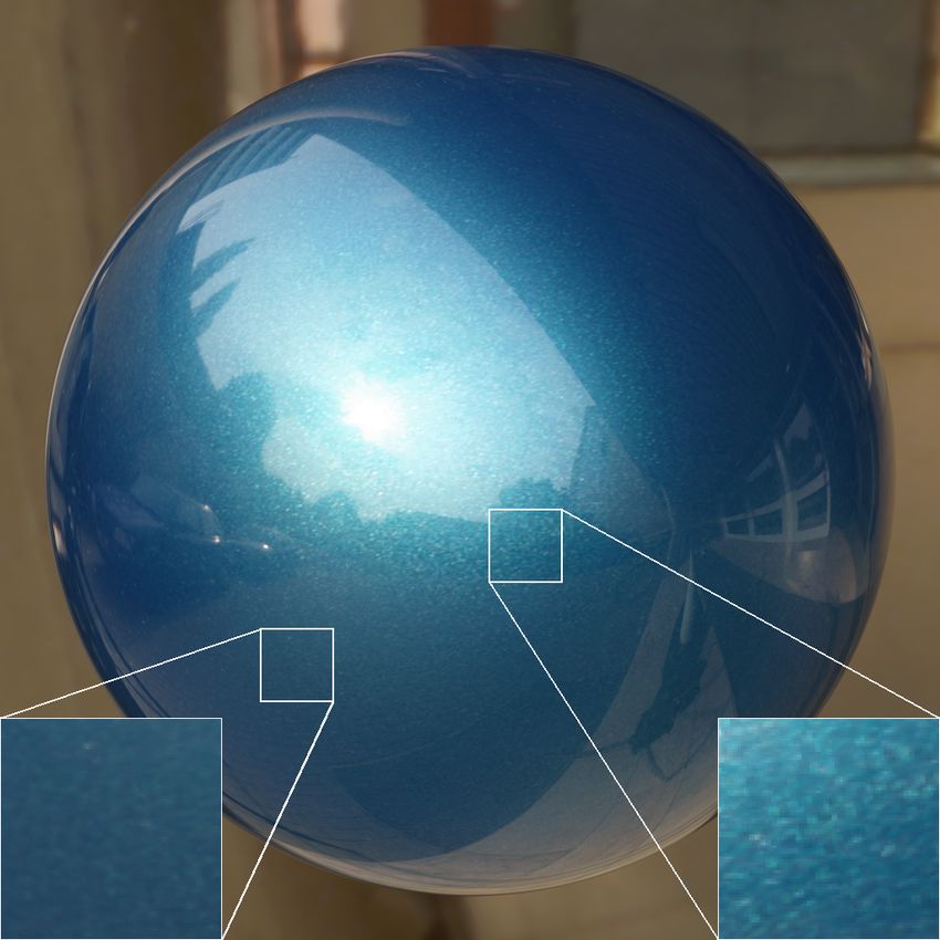
the full dataset (700x700 texels, 151x151 direc-           7    Conclusions
tions) of 62 GB. Even if this is not taken into ac-        We showed how to measure the angular frequencies
count the compression ratio of our method is more          of the glittering effects of metallic paints and how
than 7 times better than PCA for the first setting         to resample and compress measured paint data to
which is sufficient for the rendering of still images.     match the flake properties. Our method improves
Our method consumes more memory if the angular             compression ratio as well as visual quality com-
resolution is increased to match the visual impres-        pared to previous approaches like PCA.
sion of the glittering, but the ratio is still much bet-      In future work we plan to investigate the exten-
ter considering the larger amount of raw data that         sion of our example based resampling and compres-
served as input. If the data corresponding to the          sion method to a broader range of materials that are
second setting would be stored in a naive way, it          primarily defined by statistical properties.
would consume 145GB of space (720x720x50301
RGB-pixels in 16bit format). Additionally, our rep-        8    Acknowledgment
resentation conserves the sharpness of the sparkling       This work was partially supported by the German
effect much better since the PCA leads to a blur-          Science Foundation (DFG) under research grant KL
ring in spatial domain. Furthermore, PCA tends             1142/7-1.
to smear out the sparkling distribution in angular
domain when compression ratio is increased too
                                                           References
much. Zoom into Figure 6 for a visual comparison.
                                                           [1] Sergey Ershov, Andrei Khodulev, and Konstantin
  Since PCA compressed data of equal quality                   Kolchin. Simulation of sparkles in metallic paints. In
needs 20 or more principal components, the decom-              Proceedings of Graphicon ’99, pages 121–128. The
pression speed increases by a factor of about 20 be-           Eurographics Association and Blackwell Publishers,
cause our method needs only two look-ups to de-                1999.
code a certain pixel whereas the decoding speed of         [2] Johannes Günther, Tongbo Chen, Michael Goesele,
PCA is linearly dependent on the number of stored              Ingo Wald, and Hans-Peter Seidel. Efficient acqui-
                                                               sition and realistic rendering of car paint. In Vision,
components.                                                    Modeling, and Visualization 2005 (VMV’05), pages
                                                               487–494, Erlangen, Germany, November 2005. Aka.
                                                           [3] David K. McAllister, Anselmo Lastra, and Wolfgang
  D                             1208         50301             Heidrich. Efficient rendering of spatial bi-directional
                   PCA                                         reflectance distribution functions. In HWWS ’02: Pro-
  patch size                   24x24         30x30
                                                               ceedings of the ACM SIGGRAPH/EUROGRAPHICS
  spatial res-                                                 conference on Graphics hardware, pages 79–88,
                 128x128 1008x1008         720x720
  olution                                                      Aire-la-Ville, Switzerland, Switzerland, 2002. Euro-
  K                 -            16            9               graphics Association.
  λ                 -         6.24MB       81.61MB         [4] Gero Müller, Jan Meseth, and Reinhard Klein. Com-
                                                               pression and real-time rendering of measured btfs us-
  images            -        36.83MB      232.89MB             ing local pca. In Vision, Modeling and Visualisa-
  total          323MB       43.07MB      314.50MB             tion 2003, pages 271–280. Akademische Verlagsge-
  raw data       2.0GB         62GB         62GB               sellschaft Aka GmbH, Berlin, November 2003.
  ratio           1:6.3       1:1476        1:202          [5] M. Rump, G. Müller, R. Sarlette, D. Koch, and
                                                               R. Klein. Photo-realistic rendering of metallic car
Table 1: Compressed data size using different set-             paint from image-based measurements. Computer
tings for the blue-green pearlescent paint.                    Graphics Forum, 27(2):527–536, August 2008.
                                                           [6] M. Sattler, R. Sarlette, and R. Klein. Efficient and
                                                               realistic visualization of cloth. Proceedings of the Eu-
   To compare our model with still images of real              rographics Symposium on Rendering 2003, 2003.
paint we re-rendered a measured slice of the BTF.          [7] Hongcheng Wang, Qing Wu, Lin Shi, Yizhou Yu, and
Results can be taken from Figure 7. Our method is              Narendra Ahuja. Out-of-core tensor approximation
                                                               of multi-dimensional matrices of visual data. ACM
able to reproduce the original appearance of the ma-           Trans. Graph., 24(3):527–535, 2005.
terial. The compression quality can also be noticed
in Figures 6 and 8 for three representative paints
with very different brightnesses and flake densities.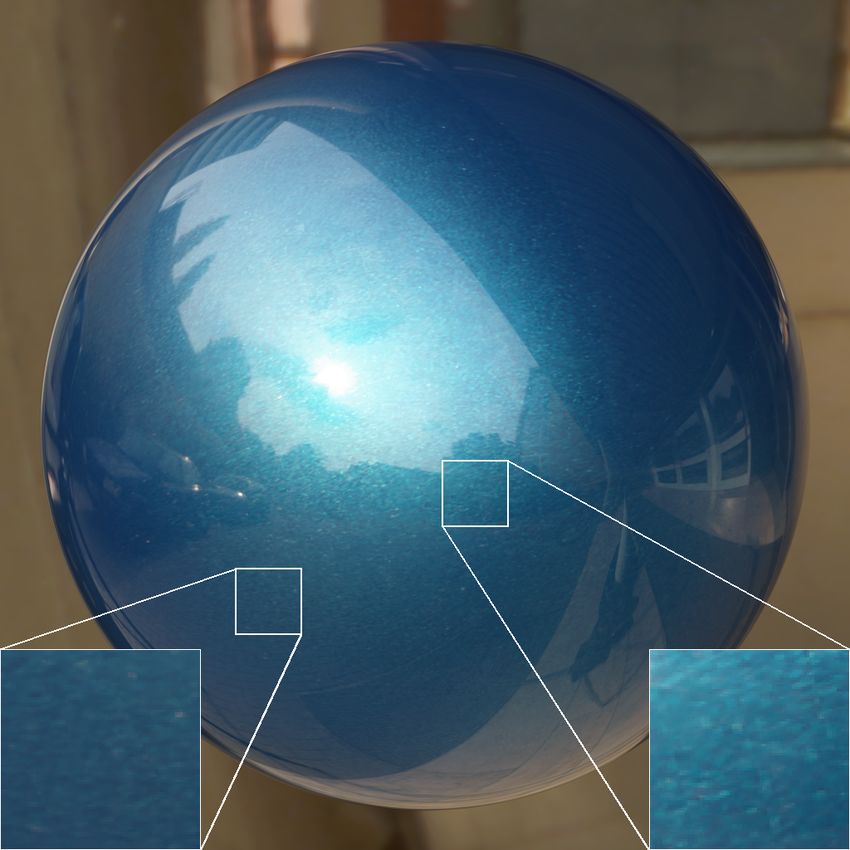
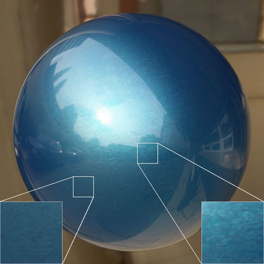
(a) uncompressed (2 GB,         (b) our method (43 MB,   (c) PCA (323 MB, 128x128)     (d) PCA (57 MB, 128x128)
  128x128 spatial resolution)            1008x1008)
Figure 6: Comparison of our technique (b) with PCA of equal quality (c) and equal size (d). (Zoom in for
comparison of sparkling effects)

              (a)Photograph (Measurement setup)                                   (b)Rendering
Figure 7: Comparison of a photograph of the blue-green pearlescent paint (a) and a rendering with our
compression method (b). The rendered paint part has been integrated into the photograph. Our method
faithfully reproduces the original flake distribution.

   (a)Uncompressed (2GB)          (b)Compressed (109MB)      (c)Uncompressed (2GB)          (d)Compressed (93MB)
Figure 8: Comparison between renderings of uncompressed data (128x128 slice) and data compressed with
our method for a dark blue metallic paint with very few and tiny flakes and a silver metallic paint with many
large flakes with a broad distribution. These images show that our method works for metallic paints with a
wide range of flake densities.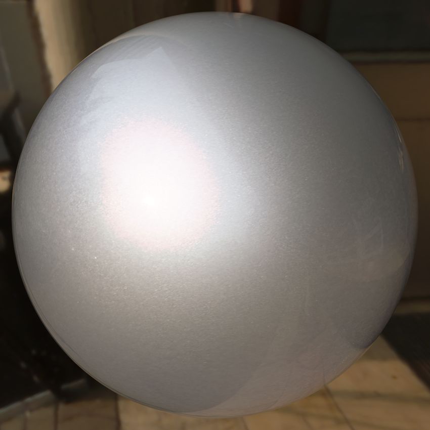
You can also read


