Learning-Driven Exploration for Reinforcement Learning
←
→
Page content transcription
If your browser does not render page correctly, please read the page content below
Learning-Driven Exploration for Reinforcement
                                                            Learning

                                                             Muhammad Usama and Dong Eui Chang

                                                School of Electrical Engineering, KAIST, Daejeon, Republic of Korea
                                                                    {usama,dechang}@kaist.ac.kr
arXiv:1906.06890v1 [cs.LG] 17 Jun 2019

                                               Abstract. Deep reinforcement learning algorithms have been shown to
                                               learn complex skills using only high-dimensional observations and scalar
                                               reward. Effective and intelligent exploration still remains an unresolved
                                               problem for reinforcement learning. Most contemporary reinforcement
                                               learning relies on simple heuristic strategies such as -greedy exploration
                                               or adding Gaussian noise to actions. These heuristics, however, are unable
                                               to intelligently distinguish the well explored and the unexplored regions
                                               of the state space, which can lead to inefficient use of training time.
                                               We introduce entropy-based exploration (EBE) that enables an agent
                                               to explore efficiently the unexplored regions of the state space. EBE
                                               quantifies the agent’s learning in a state using merely state dependent
                                               action values and adaptively explores the state space, i.e. more exploration
                                               for the unexplored region of the state space. We perform experiments
                                               on many environments including a simple linear environment, a simpler
                                               version of the breakout game and multiple first person shooter (FPS)
                                               games of VizDoom platform. We demonstrate that EBE enables efficient
                                               exploration that ultimately results in faster learning without having to
                                               tune hyperparameters.

                                               Keywords: Reinforcement Learning · Exploration · Entropy.

                                         1   Introduction

                                         Reinforcement learning (RL) is a sub-field of machine learning where an agent
                                         interacts with an environment of unknown dynamics. The objective of any RL
                                         algorithm is to learn a policy that maximizes the cumulative reward obtained
                                         by the agent. Since the agent does not begin with perfect knowledge of the
                                         environment dynamics, it has to learn solving the task through trials and errors.
                                         This gives rise to fundamental trade-off between exploration vs exploitation.
                                         Exploration is the process in which the agent learns novel information about the
                                         environment, typically through reducing its uncertainty about attainable rewards
                                         and the environment dynamics. The new knowledge acquired through exploration
                                         may offer long-term gains. In exploitation, on the other hand, the agent maximizes
                                         its reward using the knowledge it already has about the environment. A long-
                                         standing problem in RL is to find ways to achieve better trade-off between
                                         exploration and exploitation.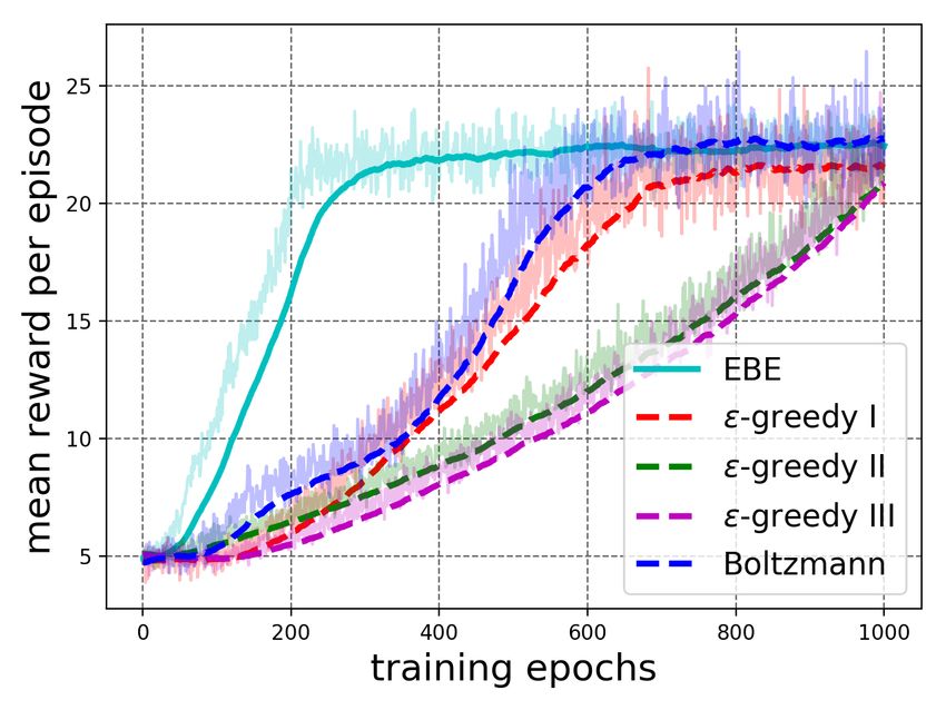
2      Muhammad Usama, Dong Eui Chang

    In this work, we argue that state dependent action values can provide valuable
information to the agent about its learning progress in a state. We use the concept
of entropy from information theory to quantify agent’s learning in a state and
subsequently make decision whether to explore in a state based on it. This
minimizes the prospects of unnecessary exploration while still exploring the
poorly explored regions of the state space.

2   Related Work

Existing entropy-based exploration strategies can be broadly divided into two
categories [1]: entropy regularization for RL and maximum entropy principle
for RL. Entropy regularization attempts to alleviate the problem of premature
convergence in policy search by imposing the information-theoretic constraints
on the learning process. In [2], authors constrain the relative entropy between old
and new state-action distributions. Some recent works including [3,4] alleviate
this problem by bounding the KL-divergence between the current and old policies.
Maximum entropy principle methods for RL aim to encourage exploration by
optimizing a maximum entropy objective. Authors in [5,6] construct this objective
by simply augmenting the conventional RL objective with entropy of the policy.
[7,8] used maximum entropy principle to make MDPs linearly solvable while [9]
employed maximum entropy principle to incorporate prior knowledge into RL
setting.
    Our proposed method belongs to the class of methods that use quantifica-
tion of uncertainty for exploration. [10] view the problem of exploration from
an information-theoretic prospective and maximizes the information that the
most recent state-action pair carries about the future. [11], on the other hand,
introduced an exploration strategy based on maximization of information gain
about the agent’s belief of the environment dynamics. Using information gain for
exploration can be traced to [12] and has been further explored in [13,10,14].
    Practical reinforcement learning algorithms often utilize simple exploration
heuristics, such as -greedy and Boltzmann exploration [15]. These methods,
however, exhibit random exploratory behavior, which can lead to exponential
regret even in the case of simple MDPs.
    Another class of exploration methods focus on predicting the environment
dynamics [16,17,18,19]. Prediction error is used as a basis of exploration and the
prediction error tends to decrease as the agent collects more information similar to
the current one about the environment dynamics. These methods, however, tend
to suffer from the noisy TV problem [19] in stochastic and partially-observable
MDPs. [19] introduced the so-called internal curiosity module to mitigate the
noisy TV problem where the focus is on predicting only those environmental
features that are relevant to the agent’s decision making.
    Our proposed method differs from entropy regularization and maximum
entropy principle methods for RL in the sense that we use entropy to quantify
agent’s learning progress in a state. Unlike imposing entropy constraints on old
and new policies in entropy regularization methods, we use entropy to decide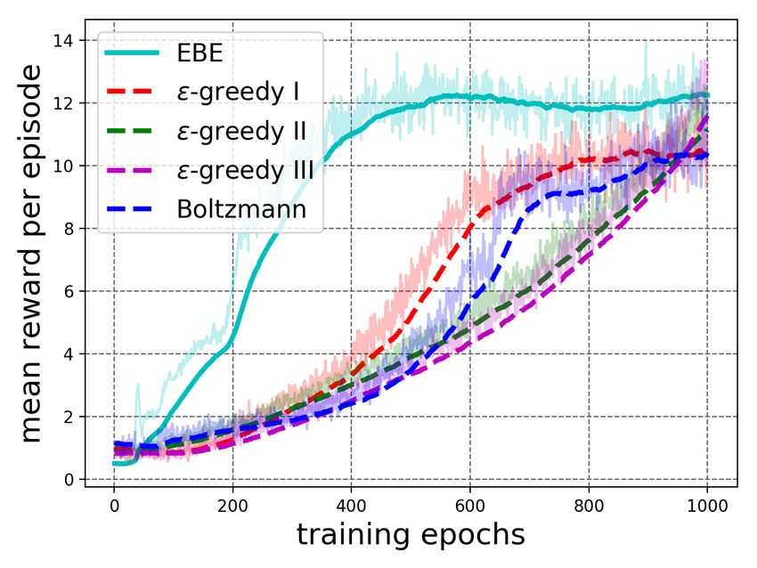
Learning-Driven Exploration for Reinforcement Learning            3

the need for exploration in a state. Still we focus on optimizing the conventional
RL objective unlike maximum entropy principle methods where the optimizable
objective is altered to improve the exploratory behavior of the agent. This allows
the agent to learn policies that obtain maximum rewards without imposing
constraints on the learning process.

3     Preliminaries
3.1   Reinforcement Learning
Reinforcement learning is a sequential decision making process in which an
agent interacts with an environment E over discrete time steps; see [15] for an
introduction. While in state st at time step t, the agent chooses an action at from
a discrete set of possible actions i.e. at ∈ A = {1, . . . , |A|} following a policy π(s)
and gets feedback in form of a scalar called reward rt following a scalar reward
function, r : S × A → R. As a result, the environment transitions into next state
st+1 according to transition probability distribution P. We denote γ ∈ (0, 1] as
discount factor and ρ0 as initial state distribution.
    The goalPof any RL algorithm is to maximize the expected discounted return
               ∞
Rt = Eπ,P [ τ =t γ τ −t rτ ] over a policy π. The policy π gives a distribution over
actions in a state.
    Following a stochastic policy π, the state dependent action value function
and the state value function are defined as

                         Qπ (s, a) = E[Rt |st = s, at = a, π],

                             V π (s) = Ea∼π(s) [Qπ (s, a)].

3.2   Deep Q-Networks in Reinforcement Learning
To approximate high-dimensional action value function given in preceding section,
we can use deep Q-network (DQN): Q(s, a; θ) with trainable parameters θ. To
train this network, we minimize the expected squared error between the target
yiDQN = r + γ maxb Q(s0 , b; θ− ) and the current network prediction Q(s, a; θi ) at
iteration i. The loss function to minimize is given as

                         Li (θi ) = E[(Q(s, a; θi ) − yiDQN )2 ],

where θ− represents the parameters of a separate target network that greatly
improves the stability of the algorithm as shown in [20]. Please see [21] for a
formal introduction to deep neural networks.

3.3   Entropy
Let us have a discrete random variable X. A discrete random variable X is
completely defined by the set X of values that it takes and its probability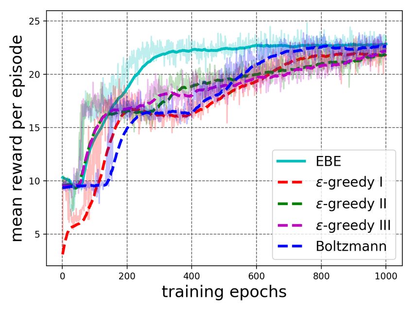
4       Muhammad Usama, Dong Eui Chang

                   (a)                                         (b)

Fig. 1. Plot of (a) mean entropy Ho , given in equation (5), and (b) accumulative
episode reward for trained, partially trained and untrained agents for 10 consecutive
test episodes. The agents are trained to play VizDoom game Seek and Destroy.

distribution {pX (x)}x∈X . Here we assume that X is a finite set, thus the random
variable X can only have finite realizations. The value pX (x) is the probability that
the random variable takes the value x. The probability distribution pX : X → [0, 1]
must satisfy the following condition
                                   X
                                        pX (x) = 1.
                                  x∈X

The entropy HX of a discrete random variable X with probability distribution
pX (x) is defined as

                                    X
                          HX = −          pX (x) logb pX (x)
                                    x∈X
                               = −EX∼pX [logb pX (x)],

    where the logarithm is taken to the base b and we define by continuity that
0 logb 0 = 0.
Intuitively, entropy quantifies the uncertainty associated with a random variable.
The greater the entropy, the greater is the surprise associated with realization of
a random variable.

4    Entropy-Based Exploration (EBE)

In this section, we explain the proposed entropy-based exploration (EBE) method.
First we go through the motivation behind EBE and then we present the mathe-
matical realization for the concept.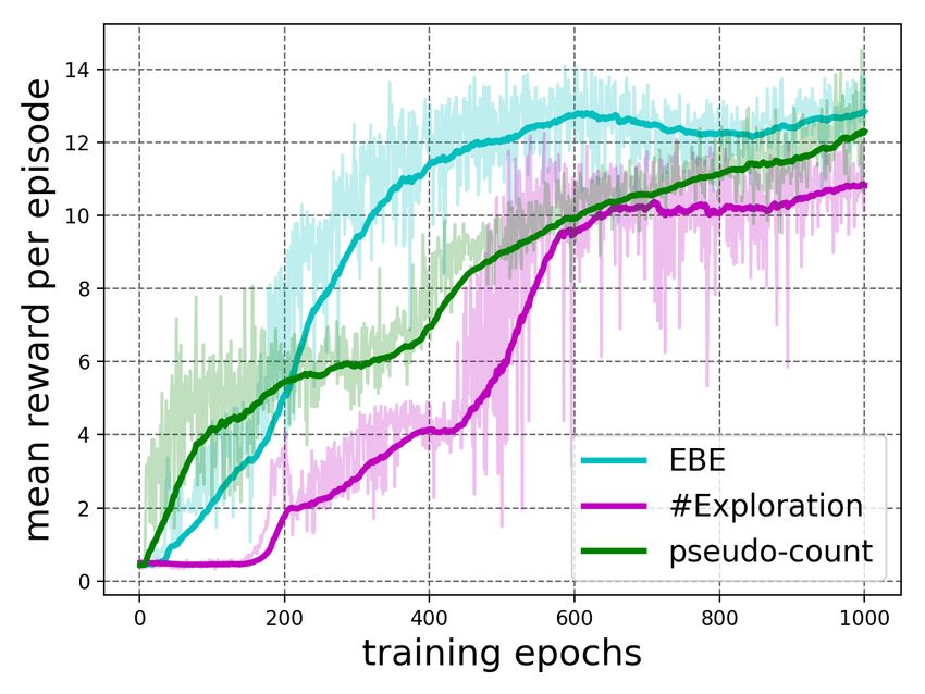
Learning-Driven Exploration for Reinforcement Learning        5

               Fig. 2. Concept behind entropy-based exploration (EBE).

4.1     Motivation

Usually in RL training, the agent has gathered more knowledge in well explored
region of the state space. The lack of knowledge in unexplored states is a result
of insufficient learning in those states. Therefore, an effective exploration strategy
should adapt itself to explore more in states where the agent has performed
less learning, which we refer to as learning-driven exploration. Learning-driven
exploration enables the agent to perform more exploration in poorly explored
regions of state space, which usually occur at the later stages of training episode.
This allows the agent to explore deeper into the state space resulting into deep1
exploration. Our definition of deep exploration is different from [22] where deep
exploration means ”exploration which is directed over multiple time steps or
far-sighted exploration” [22]. In our work, Deep exploration concerns spatially
extended exploration in the state space. The concept is illustrated in Figure 2.
As the training process continues, the well explored region of the state space
increases. Figure 2 shows two different training trajectories, related to EBE
and -greedy exploration, at three different instances in the presumed learning
process. The redness of a trajectory indicates the exploration probability in that
state. For EBE, the exploration probability is small in well explored region of the
state space and it increases as we get closer to unexplored region. This enables
the agent to explore adaptively based on its learning in a state, resulting in
deep exploration. But for -greedy exploration where value of  is annealed from
the start to the end of the training process, at a particular instant in learning
process, the agent explores in all states with the same probability irrespective of
its learning in those states. Adaptive exploration by EBE enables the agent to
allocate more resources towards exploring poorly understood regions of the state
space, thus improving the learning progress.

1
    word deep is used here in different context from deep learning.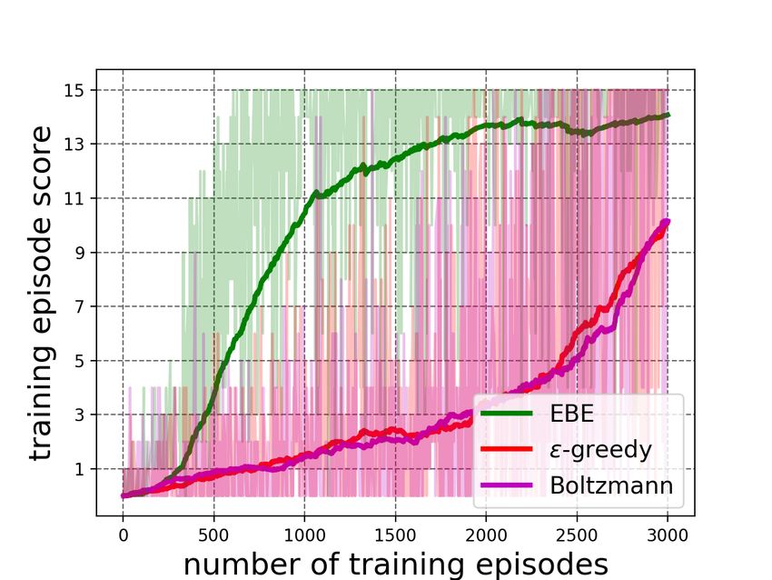
6       Muhammad Usama, Dong Eui Chang

4.2   Entropy-Based Exploration (EBE): A Realization of
      Learning-Driven Deep Exploration
The agent quantifies the utility of an action in a state in the form of state
dependent Q-values. We can use the difference between Q-values in a state as an
estimate of agent’s learning progress in that state. Therefore, we use Q-values to
define a probability distribution over actions in a state, i.e.

                                            eQ(s,a)
                              ps (a) = P         Q(s,b)
                                                        ,                       (1)
                                           b∈A e

where A is the set of all possible actions in state s. Here we note that eQ(s,a) may
cause numerical overflow when Q(s, a) is large. To improve numerical stability,
we use the so-called max trick. We thus have
                                         eQ(s,a)−Qo (s)
                           ps (a) = P         Q(s,b)−Qo (s)
                                                            ,                   (2)
                                        b∈A e

where Qo (s) = maxã∈A Q(s, ã). This improves the numerical stability while
keeping the distribution ps (a) unchanged. We then use ps (a) to obtain state
dependent entropy, H̃(s), as follows
                                   X
                        H̃(s) = −     ps (a) logb ps (a),                 (3)
                                    a∈A

where b > 0 is the base of logarithm. We note that H̃(s) may be greater than 1
when |A| > b, therefore, we normalize H̃(s) between 0 and 1. Since maximum
value the entropy can take is logb (|A|), we define a scaled entropy H(s) ∈ [0, 1]
as follows:
                                   P
                                 − a∈A ps (a) logb ps (a)
                        H(s) =
                                         logb (|A|)
                                   X
                              =−       ps (a) log|A| ps (a).                  (4)
                                   a∈A

H(s) in equation (4) quantifies the agent’s learning in state s: the lower the
entropy H(s), the more learned the agent is that some actions are better than
others. Therefore, we use H(s) to guide exploration in a state: greater the
value of H(s), more is the need for exploration. Given H(s) in a state from
equation (4), the agent explores with probability H(s) i.e. it behaves randomly.
In practice, entropy-based exploration is similar to -greedy exploration method
with  replaced with state dependent H(s).

How does entropy estimate agent’s learning in a state? To see how
entropy can estimate agent’s learning in a state, we see that state space can be
broadly classified into two categories: states in which choice of action is crucial
and states in which choice of action does not significantly impact what happens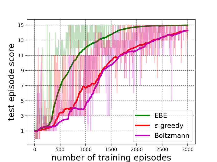
Learning-Driven Exploration for Reinforcement Learning          7

in the future [23]. For later states, some actions are decisively better than others.
Quantitatively, it means that Q-values for better actions are significantly higher
than Q-values of the remaining actions. Therefore, the distribution defined in
equation (2) is highly skewed towards better actions and by equation (4), the
entropy of these states is low. Note that the lowest achievable entropy may be
different for different states.
    Consider, for example, the case where the agent is trained to play VizDoom
game Seek and Destroy. The details about the environment and experimental
setup are given in Section 5.3. We consider three cases comprised of an untrained
agent2 , a partially trained agent3 and a trained agent4 . Here, we define Ho ∈ [0, 1]
as entropy averaged over an entire episode, i.e.

                                          N
                                       1 X
                                Ho =         H(si ),                              (5)
                                       N i=1

where N is the number of steps in the episode, si represents state at ith step and
H(si ) gives entropy of si as defined in equation (4). We test the agents for 10
consecutive episodes. Figure 1 plots Ho and accumulated episode reward versus
test episodes. We see in Figure 1(a) that Ho is lowest for trained agent for all
episodes. Also the trained agent obtains the highest accumulative reward in all
episodes as shown in 1(b). The partially trained agent still has significant Ho
values for all episodes which reflects its incomplete learning.
    These results show that entropy is a good measure to estimate agent’s learning
in a state, which in turn can be used to quantify the need for exploration. This
forms the base for our proposed entropy-based exploration strategy.
    It is worthwhile to note that for states where all available actions have
similar Q-values, the entropy remains close to 1 irrespective of learning progress.
Therefore, entropy does not reflect the agent’s learning in these states. This,
however, does not affect the learning process as choice of action is practically
irrelevant in these states owing to similar Q-values as mirrored by experiments
in Section 5.

5     Experiments

We demonstrate the performance of EBE on many environments including a
linear environment, a simpler breakout game and multiple FPS games of Vizdoom
[25]. Results shown are averaged over five runs. Please note that all appendices
are placed in supplementary material due to limited space. Code to reproduce the
experiments is given at: https://github.com/Usama1002/EBE-Exploration.
2
    the Q-network was initialized using Kaiming Uniform method [24] and no further
    training was performed.
3
    the agent was trained using EBE for two epochs only.
4
    the agent was trained using EBE for 20 epochs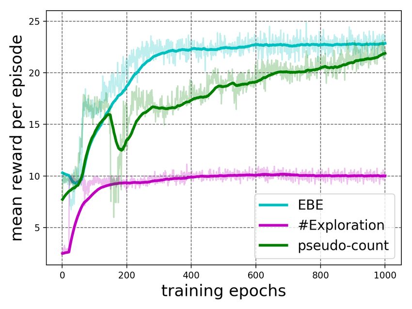
8       Muhammad Usama, Dong Eui Chang

                    (a)                                (b)

Fig. 3. (a) Simple linear environment consists of 21 states. Episode starts in state
s = 10, shown in red circle. States s = 0 and s = 20, shown in green rounded rectangles,
are terminal states. For non-terminal states, the agent can transition into either of its
neighboring states. The agent gets reward r = 1 for transitioning into the terminal
states and zero reward otherwise. (b) Squared Error loss for value iteration task on
linear environment.
5.1   Value Iteration on Simple Linear Environment
We start our experiments by measuring the performance of EBE on a simple
value iteration task. The reason for choosing this task is that it is devoid of
many confounding complexities and provides better insight into used methods.
Moreover, exact optimal Q-values, Q∗ (s, a) for all (s, a) ∈ (S × A), can be
computed analytically which helps monitor the learning progress.
    The environment is described in Figure 3(a). We use temporal difference
based tabular Q-learning without eligibility traces to learn the optimal Q-values,
Q(s, a) for all (s, a) ∈ (S × A).
    As baselines, we use -greedy exploration where  value is linearly annealed
from 1.0 to 0.0 over the number of episodes and Boltzmann exploration where
the temperature is linearly decreased from 0.8 to 0.1. Agents are trained for 200
episodes with maximum episode length of 50 steps. Optimal steps to successfully
reaching a rewarding state are 10. Values for discount factor and learning rate
are 0.9 and 0.2 respectively. The evaluation metric is mean squared error between
the actual Q-values, Q∗ (s, a), and the learned Q-values, Q(s, a):
                                X
                          L=         (Q∗ (s, a) − Q(s, a))2 .
                              s∈S,a∈A

The squared error is plotted in Figure 3(b). We see that Q-values learnt with
EBE converge to optimal Q-values while others fail. This is a very promising
result as it indicates the ability of EBE to adequately explore the state space.

5.2   A Simpler Breakout Game
We experiment with a simpler breakout game whose state space is much simpler
than that of Breakout game of Atari suite that allows detailed analysis of employed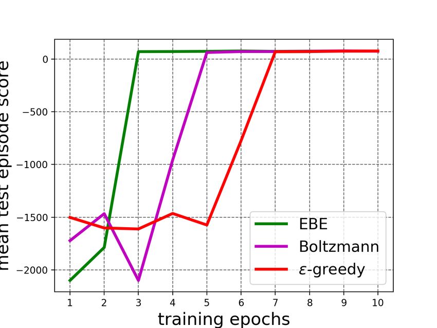
Learning-Driven Exploration for Reinforcement Learning         9

                   (a)                                       (b)

Fig. 4. Plots show (a) test episode scores and (b) training episode scores for agents
trained with EBE, -greedy exploration and Boltzmann exploration on simpler breakout
game. Smoothed data is shown with solid lines while unsmoothed data is ghosted in
the background. Smoothing method is adopted from [26] with weight 0.99.

methods, yet it is complex enough to offer significant learning challenge as it uses
a neural network as function approximator and works on raw images as states.
There are 15 bricks to break and the agent is rewarded 1 point for breaking each
brick. Episode ends when one of the following happens: all bricks are broken, the
paddle misses the ball or the maximum steps limit has reached. We use a stack
of 2 images, the current image and the previous images, as our state observation.
In any state, the agent can either move the paddle left, move it right or leave it
still. EBE is compared to -greedy exploration in which  is linearly annealed
from 1.0 to 0.0 over the number of episodes and Boltzmann exploration where
temperature is linearly annealed from 1.0 to 0.01 over training process. Please
see Appendix A for details regarding the experimental setup.
    The results are shown in Figure 4. We see that agent trained with EBE
learns much faster than those trained with -greedy and Boltzmann exploration
strategies, as shown in Figure 4(a). Figure 4(b) plots the training episode rewards
versus the episode numbers. We see that for EBE, the agent starts performing
high reward training episodes from the very start of training process, while
training episode rewards for the agents trained with -greedy and Boltzmann
exploration increase steadily. This validates our hypothesis of deep exploration,
in which the agent transitions quickly into the poorly explored region of the state
space, which usually corresponds to the later states of a training episode.

5.3   VizDoom
We use VizDoom platform [25] to conduct experiments and compare EBE with
-greedy exploration.

Seek and Destroy The environment consists of grey walls, ceiling and floor.
The agent is placed in the center of wall and a monster is spawned randomly on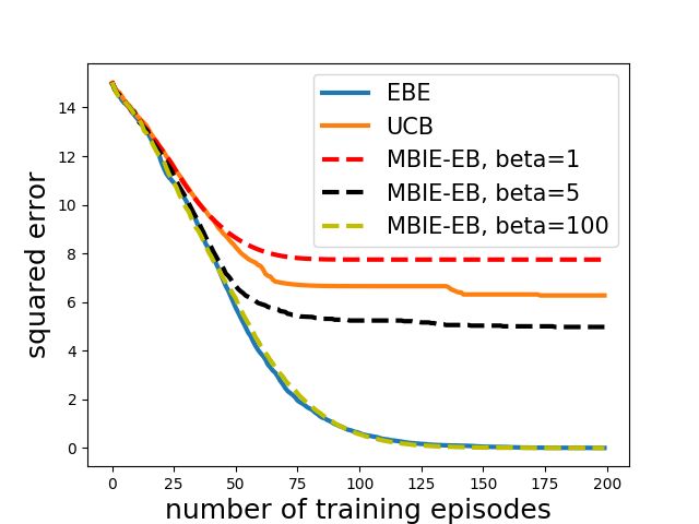
10      Muhammad Usama, Dong Eui Chang

                   (a)                                       (b)

Fig. 5. Performance of agents trained with entropy-based exploration (EBE), Boltz-
mann exploration and -greedy exploration strategy on VizDoom game Seek and Destroy.
(a) plots mean test score of 100 test episode scores played after each training epoch
while (b) plots mean score of all training episodes played in a training epoch.

the opposite wall. The agent is tasked to kill the monster with its gun. The gun
can only fire straight, so the agent must come in line with the monster before
firing a shot. Reward of 101 points is given for killing the monster. Penalty of
5 points is given for each missed shot, therefore optimal agent should kill the
monster with only one shot. Penalty of 1 point is given for each step taken to
motivate the agent to kill the monster faster.
    The state space is partially observable to the agent via raw images. The agent
can either move left, move right or attack in a state. The episode ends when
either of the following happens: the monster is dead, player is dead or 300 time
steps have passed.
    We compare EBE with Boltzmann and -greedy exploration strategies. In
Boltzmann exploration, the temperature parameter is linearly annealed from 1.0
to 0.01 over the training epochs. For -greedy exploration,  is set to 1.0 for first
epoch, then  is linearly annealed to 0.01 till epoch 6. Thereafter,  = 0.01 is
used. Please see Appendix A for further details about the training setup.
    The results are shown in Figure 5. Mean test scores in Figure 5(a) show
that agent trained with EBE outperforms the agents trained with Boltzmann
and -greedy exploration. Similarly, we see in Figure 5(b) that EBE exploration
results in high reward training episodes considerably earlier in training that
manifests deep exploration as defined in Section 4.1.

Defend the Center This environment consists of a circular map in which the
agent is placed in the middle and monsters are spawned around it. To stay alive,
the agent has to kill the monsters around it. The player can only rotate about its
position. The player is rewarded one point for each kill and penalized one point
for being killed. The agent is provided with 26 ammo, so it should learn to use
the ammunition wisely to kill as many monsters as possible before being dead
itself.
Learning-Driven Exploration for Reinforcement Learning 11
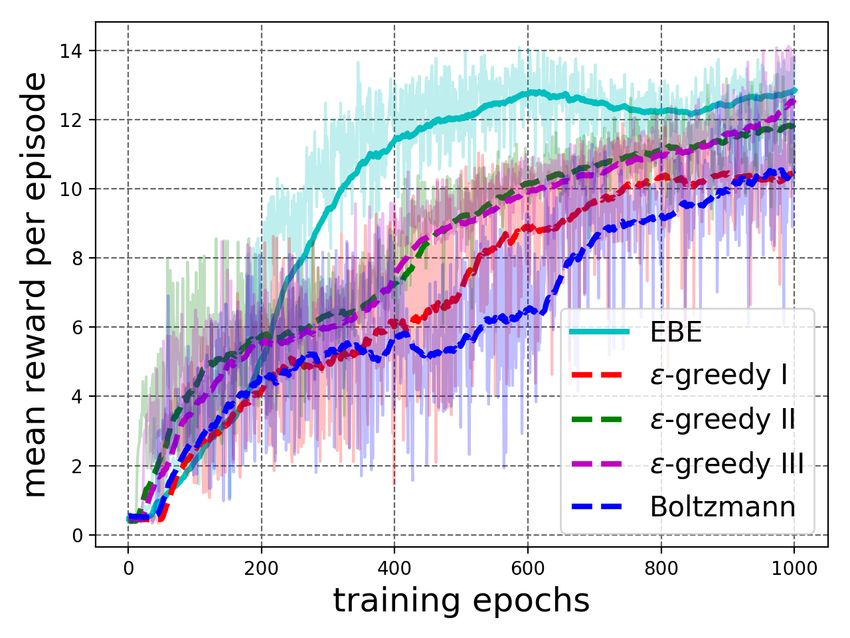
Table 1. Variants of baseline -greedy exploration strategy.
variant details
=1.0 is used for first 100 epochs, then it is linearly annealed to 0.01
-greedy I
till 600 epochs. Afterwards =0.01 is used.
-greedy II is linearly annealed from 1.0 to 0.01 over the entire training process.
= 1.0 is used for first 100 epochs. is then linearly annealed from 1.0
-greedy III
to 0.01 over the remaining training process.
(a) (b)
Fig. 6. Plot of (a) mean test reward and (b) mean training reward per episode of
agents trained with EBE, -greedy and Boltzmann exploration strategies on VizDoom
game Defend the Center. Plots show smoothed data while unsmoothed data is ghosted
in the background. Smoothing method is adopted from [26] with weight 0.975.
The episode ends when the agent is dead or 2100 steps (60 seconds) have
passed. The agent observes the state using raw frames and can either attack,
turn left and turn right in a state. An episode is considered successful if the agent
kills at least 11 monsters before being dead itself, i.e. score at least 10 points.
We compare EBE with -greedy and Boltzmann exploration. We use three
different variants of -greedy exploration which are detailed in Table 1. For
Boltzmann exploration, the temperature parameter is linearly annealed from 1.0
to 0.01 over the learning process. The agents are trained for 1000 epochs and
each epoch consists of 5000 steps. 100 consecutive test episodes are played after
each epoch. Details about the experimental setup are given in Appendix A.
The experimental results are shown in Figure 6 where (a) plots mean test
rewards obtained by taking the mean of 100 test episodes after each epoch and
(b) plots mean training reward obtained by taking the mean of all training
episode rewards in an epoch. We see in Figure 6(a) that agent trained with
EBE exploration attains the maximum mean test reward per episode after about
60% of training epochs as compared to other exploration strategies. Moreover,
Figure 6(b) shows deep exploration, defined in Section 4.1, where EBE was able
to perform high reward training episodes early on in the training process. This12 Muhammad Usama, Dong Eui Chang
(a) (b)
Fig. 7. Plot of (a) mean test reward and (b) mean training reward per episode of
agents trained with EBE, -greedy and Boltzmann exploration strategies on VizDoom
game Defend the Line. Plots show smoothed data while unsmoothed data is ghosted in
the background. Smoothing method is adopted from [26] with weight 0.975.
result shows effectiveness of EBE on high-dimensional RL task that enables
effective exploration without having to tune any hyperparameters.
Defend the Line This environment is similar to defend the center except that
the map is rectangular with the agent placed on one side and monsters spawning
on the opposite wall. The agent is rewarded one point for each kill and penalized
one point for being dead. Here, the agent is provided with unlimited ammunition
and limited health that decreases with each attack the agent takes from the
monsters. The agent observes raw frames and can attack, turn left or turn right
in a state. The episode ends when the agent is dead or episode times out with
2100 steps (60 seconds). The goal is to kill at least 16 monsters before the agent
dies, i.e. to obtain at least 15 points in one episode. EBE is compared to the
same baselines as considered in Section 5.3. Details about the experimental setup
are given in Appendix A.
The experimental results are shown in Figure 7 where, similar to Figure 6,
(a) plots mean test rewards per episode and (b) plots mean training reward
per episode. Figure 7(a) that agent trained with EBE exploration attains the
maximum mean test reward per episode after about 30% of training epochs
as compared to other exploration strategies. Moreover, Figure 7(b) shows deep
exploration, defined in Section 4.1, where EBE was able to perform high reward
training episodes early on in the training process. This result shows that EBE
performs effective exploration on high-dimensional RL tasks without having to
tune any hyperparameters.
5.4 Comparison of EBE with Count-Based Exploration Methods
Some of the classic and theoretically-justified exploration methods are based on
counting state-action visitations and turning this count into a bonus reward toLearning-Driven Exploration for Reinforcement Learning 13
(a) (b)
Fig. 8. (a) Comparison of EBE with UCB and MBIE-EB on linear environment.
(b) Comparison of EBE with #Exploration and pseudo-count based exploration on
VizDoom game Seek and Destroy.
guide exploration. In the bandit setting, the widely-known Upper-Confidence-
q
2 log t
Bound (UCB) [27] chooses the action at that maximizes r̂(at ) + N (at ) where
r̂(at ) is the estimated reward of executing at and N (at ) is the number of times
the action at was previously chosen. Similar algorithms have been proposed for
MDP setting that favor the selection of less visited state-action pairs by selecting
the action at at time t that maximizes c̃(st , at ) = Q(st , at ) + B(N (st , at )) where
N (st , at ) is the number of times the pair (st , at ) was previously visited. Here,
B(N (st , at )) is the exploration bonus that decreases with the increase in N (st , at ).
Model Based Interval Estimation-Exploration Bonus (MBIE-EB) [28] proposed
using exploration bonus of the form B(N (st , at )) = √ β , where β is a
N (st ,at )
constant. Analogous
q to UCB for bandit-setting, we can get exploration bonus
2 log t
B(N (st , at )) = N (st ,at ) for MDPs. We compare our proposed method EBE
with UCB and MBIE-EB on linear MDP environment considered previously
in Section 5.1 under the same experiments settings. As shown in Figure 8(a),
EBE performs better than UCB in terms of convergence. The performance of
MBIE-EB imporves as value of β is increased and with β = 100, the performance
of MBIE-EB becomes comparable to EBE.
MBIE-EB, UCB and related algorithms assume that the MDP is solved
analytically at each timestep, which is only practical for small finite state spaces.
Therefore, counting-based methods cannot be extended to high-dimensional,
continuous state spaces as visit counts are not directly useful in large domains,
where states are rarely visited more than once. [29] addressed this issue by
deriving pseudo-counts from arbitrary density models over the state space and
allow generalization of count-based exploration algorithms to the non-tabular
case. #Exploration algorithm [30] uses hashing to discretize the high-dimensional
state space whereby the states are mapped to hash codes which allows to count
their visitations using a hash table. This visitation count is then used to compute
the exploration bonus using the classic count-based exploration theory.14 Muhammad Usama, Dong Eui Chang
(a) (b)
Fig. 9. (a) Comparison of EBE with #Exploration and pseudo-count based exploration
methods on VizDoom games (a) defend the center and (b) defend the line.
We compare EBE with pseudo-count based exploration algorithm [29] and
#Exploration [30]. Please see Appendix B for implementation details of these
baselines. Figure 8(b) shows the results for VizDoom game Seek and Destroy.
EBE and #Exploration are able to learn solving the task with EBE learning much
earlier while pseudo-count algorithm failed to solve the task. Similarly, Figure
9(a) and Figure 9(b) show comparison results for defend the center and defend
the line, respectively. For both games defend the center and defend the line, EBE
depicts efficient exploration by learning to solve the tasks with higher rewards
much earlier than the baselines. However, #Exploration strategy settles at much
lower score for both the games. Table 2 provides the wall time averaged across
all runs for the considered exploration strategies for DTC and DTL. -greedy
is the most efficient in terms of wall time, followed by EBE. The exceptionally
higher wall time required for #Exploration strategy can be explained by the
online training of the autoencoder used for generating the hash codes.
Table 2. Wall time in hours averaged across five runs for various exploration strategies.
environment EBE -greedy Boltzmann #Exploration pseudo-count
defend the center 39 38 42.5 64 51.5
defend the line 40 38 44 61.5 52
In conclusion, the proposed entropy-based exploration (EBE) method is able
to achieve remarkable performance on tabular as well as on high-dimensional
environments including various VizDoom games and a simpler breakout game.
EBE is also efficient in terms of wall time and performs comparable to -greedy
exploration.Learning-Driven Exploration for Reinforcement Learning 15
6 Conclusion
We have introduced a simple to implement yet effective exploration strategy
that intelligently explores the state space based on agent’s learning. We show
that entropy of state dependent action values can be used to estimate agent’s
learning for a set of states. Based on agent’s learning, the proposed entropy-based
exploration (EBE) is able to decipher the need for exploration in a state, thus,
exploring more the unexplored region of state space. This results into what we
call deep exploration which is confirmed by multiple experiments on diverse
platforms. As shown by the experiments, EBE results into faster and better
learning on tabular and high-dimensional state space platforms without having
to tune any hyperparameters.
References
1. Zhang-Wei Hong, Tzu-Yun Shann, Shih-Yang Su, Yi-Hsiang Chang, Tsu-Jui Fu,
and Chun-Yi Lee. Diversity-driven exploration strategy for deep reinforcement
learning. In S. Bengio, H. Wallach, H. Larochelle, K. Grauman, N. Cesa-Bianchi,
and R. Garnett, editors, Advances in Neural Information Processing Systems 31,
pages 10510–10521. Curran Associates, Inc., 2018.
2. Jan Peters, Katharina Mülling, and Yasemin Altun. Relative entropy policy search.
In AAAI 2010, 2010.
3. John Schulman, Sergey Levine, Pieter Abbeel, Michael Jordan, and Philipp Moritz.
Trust region policy optimization. In Francis Bach and David Blei, editors, Pro-
ceedings of the 32nd International Conference on Machine Learning, volume 37 of
Proceedings of Machine Learning Research, pages 1889–1897, Lille, France, 07–09
Jul 2015. PMLR.
4. John Schulman, Filip Wolski, Prafulla Dhariwal, Alec Radford, and Oleg Klimov.
Proximal policy optimization algorithms. CoRR, abs/1707.06347, 2017.
5. Brian D. Ziebart and Martial Hebert. Modeling purposeful adaptive behavior with
the principle of maximum causal entropy, 2010.
6. Tuomas Haarnoja, Aurick Zhou, Pieter Abbeel, and Sergey Levine. Soft actor-critic:
Off-policy maximum entropy deep reinforcement learning with a stochastic actor.
CoRR, abs/1801.01290, 2018.
7. Emanuel Todorov. Linearly-solvable markov decision problems. In B. Schölkopf,
J. C. Platt, and T. Hoffman, editors, Advances in Neural Information Processing
Systems 19, pages 1369–1376. MIT Press, 2007.
8. Emanuel Todorov. Compositionality of optimal control laws. In NIPS, 2009.
9. Roy Fox, Ari Pakman, and Naftali Tishby. Taming the noise in reinforcement
learning via soft updates. In Proceedings of the Thirty-Second Conference on
Uncertainty in Artificial Intelligence, UAI’16, pages 202–211, Arlington, Virginia,
United States, 2016. AUAI Press.
10. Susanne Still and Doina Precup. An information-theoretic approach to curiosity-
driven reinforcement learning. Theory in Biosciences, 131(3):139–148, Sep 2012.
11. Rein Houthooft, Xi Chen, Yan Duan, John Schulman, Filip De Turck, and Pieter
Abbeel. Curiosity-driven exploration in deep reinforcement learning via bayesian
neural networks. CoRR, abs/1605.09674, 2016.
12. Jan Storck, Sepp Hochreiter, and Jrgen Schmidhuber. Reinforcement driven infor-
mation acquisition in non-deterministic environments, 1995.16 Muhammad Usama, Dong Eui Chang
13. Yi Sun, Faustino J. Gomez, and Jürgen Schmidhuber. Planning to be surprised:
Optimal bayesian exploration in dynamic environments. CoRR, abs/1103.5708,
2011.
14. Daniel Y. Little and Friedrich T. Sommer. Learning and exploration in action-
perception loops. In Front. Neural Circuits, 2013.
15. Richard S. Sutton and Andrew G. Barto. Reinforcement learning - an introduction.
Adaptive computation and machine learning. MIT Press, 1998.
16. Jürgen Schmidhuber. A possibility for implementing curiosity and boredom in model-
building neural controllers. In Proceedings of the First International Conference
on Simulation of Adaptive Behavior on From Animals to Animats, pages 222–227,
Cambridge, MA, USA, 1990. MIT Press.
17. Bradly C. Stadie, Sergey Levine, and Pieter Abbeel. Incentivizing exploration in
reinforcement learning with deep predictive models. CoRR, abs/1507.00814, 2015.
18. Joshua Achiam and Shankar Sastry. Surprise-based intrinsic motivation for deep
reinforcement learning. CoRR, abs/1703.01732, 2017.
19. Deepak Pathak, Pulkit Agrawal, Alexei A. Efros, and Trevor Darrell. Curiosity-
driven exploration by self-supervised prediction. In ICML, 2017.
20. Volodymyr Mnih, Koray Kavukcuoglu, David Silver, Andrei A. Rusu, Joel Veness,
Marc G. Bellemare, Alex Graves, Martin Riedmiller, Andreas K. Fidjeland, Georg
Ostrovski, Stig Petersen, Charles Beattie, Amir Sadik, Ioannis Antonoglou, Helen
King, Dharshan Kumaran, Daan Wierstra, Shane Legg, and Demis Hassabis. Human-
level control through deep reinforcement learning. Nature, 518(7540):529–533,
February 2015.
21. Anthony L. Caterini and Dong Eui Chang. Deep Neural Networks in a Mathematical
Framework. Springer Publishing Company, Incorporated, 1st edition, 2018.
22. Ian Osband, Charles Blundell, Alexander Pritzel, and Benjamin Van Roy. Deep
exploration via bootstrapped dqn. In D. D. Lee, M. Sugiyama, U. V. Luxburg,
I. Guyon, and R. Garnett, editors, Advances in Neural Information Processing
Systems 29, pages 4026–4034. Curran Associates, Inc., 2016.
23. Ziyu Wang, Tom Schaul, Matteo Hessel, Hado Van Hasselt, Marc Lanctot, and
Nando De Freitas. Dueling network architectures for deep reinforcement learning.
In Proceedings of the 33rd International Conference on International Conference
on Machine Learning - Volume 48, ICML’16, pages 1995–2003. JMLR.org, 2016.
24. Kaiming He, Xiangyu Zhang, Shaoqing Ren, and Jian Sun. Delving deep into
rectifiers: Surpassing human-level performance on imagenet classification. CoRR,
abs/1502.01852, 2015.
25. Michal Kempka, Marek Wydmuch, Grzegorz Runc, Jakub Toczek, and Wojciech
Jaskowski. Vizdoom: A doom-based AI research platform for visual reinforcement
learning. CoRR, abs/1605.02097, 2016.
26. William Chargin and Dan Moré. Tensorboard smoothing im-
plementation. https://github.com/tensorflow/tensorboard/blob/
f801ebf1f9fbfe2baee1ddd65714d0bccc640fb1/tensorboard/plugins/scalar/
vz_line_chart/vz-line-chart.ts#L704, 2015.
27. Tze Leung Lai and Herbert Robbins. Asymptotically efficient adaptive allocation
rules. Advances in Applied Mathematics, 6(1):4-22, 1985.
28. Tze Leung Lai and Herbert Robbins. An analysis of model-based interval estimation
for markov decision processes. Journal of Computer and System Sciences, 74(8):1309-
1331, 2008.
29. Marc G. Bellemare, Sriram Srinivasan, Georg Ostrovski, Tom Schaul, David Saxton,
and Rémi Munos. Unifying count-based exploration and intrinsic motivation. CoRR,
abs/1606.01868, 2016.Learning-Driven Exploration for Reinforcement Learning 17
30. Haoran Tang, Rein Houthooft, Davis Foote, Adam Stooke, Xi Chen, Yan Duan,
John Schulman, Filip De Turck, and Pieter Abbeel. #exploration: A study of
count-based exploration for deep reinforcement learning. CoRR, abs/1611.04717,
2016.You can also read