Lawrence Berkeley National Laboratory - Recent Work - eScholarship
←
→
Page content transcription
If your browser does not render page correctly, please read the page content below
Lawrence Berkeley National Laboratory
Recent Work

Title
Do optimization methods in deep learning applications matter?

Permalink
https://escholarship.org/uc/item/7gm0h48h

Authors
Ozyildirim, Buse Melis
Kiran, Mariam

Publication Date
2020

Peer reviewed

 eScholarship.org                                Powered by the California Digital Library
                                                                 University of California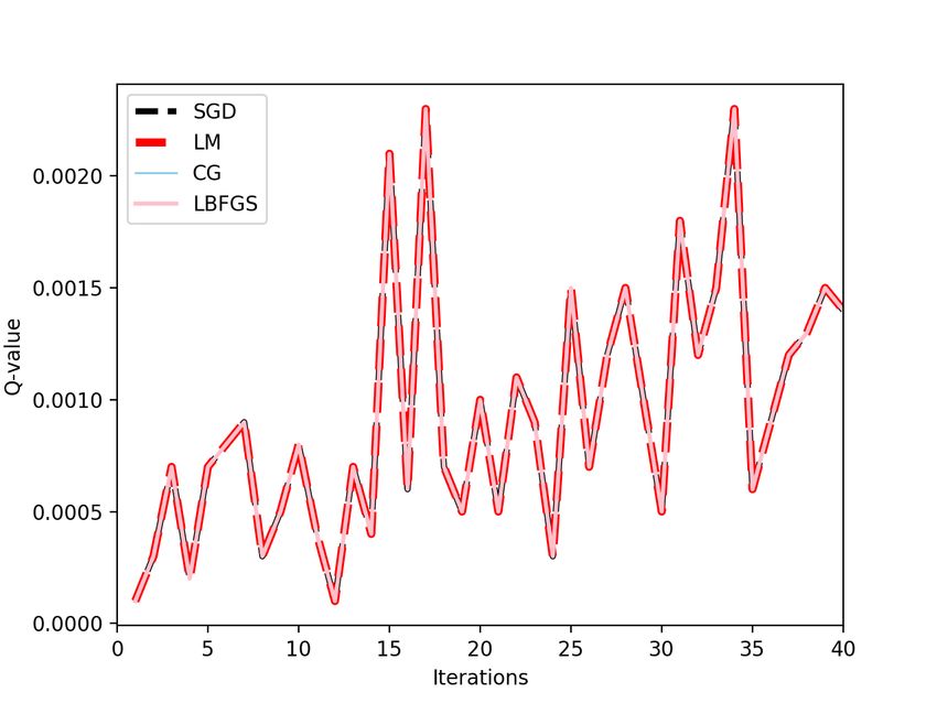
D O O PTIMIZATION M ETHODS IN D EEP L EARNING
                                                                  A PPLICATIONS M ATTER ?

                                                                                              A P REPRINT

                                                           Buse Melis Ozyildirim                                   Mariam Kiran
                                                       Department of Computer Science                          Energy Sciences Network
arXiv:2002.12642v1 [cs.LG] 28 Feb 2020

                                                            Cukurova University                          Lawrence Berkeley National Laboratory
                                                               Adana, Turkey                                        Berkeley, CA
                                                         mozyildirim@cu.edu.tr                                     mkiran@es.net

                                                                                             March 2, 2020

                                                                                             A BSTRACT
                                                  With advances in deep learning, exponential data growth and increasing model complexity, developing
                                                  efficient optimization methods are attracting much research attention. Several implementations favor
                                                  the use of Conjugate Gradient (CG) and Stochastic Gradient Descent (SGD) as being practical and
                                                  elegant solutions to achieve quick convergence, however, these optimization processes also present
                                                  many limitations in learning across deep learning applications. Recent research is exploring higher-
                                                  order optimization functions as better approaches, but these present very complex computational
                                                  challenges for practical use. Comparing first and higher-order optimization functions, in this paper,
                                                  our experiments reveal that Levemberg-Marquardt (LM) significantly supersedes optimal convergence
                                                  but suffers from very large processing time increasing the training complexity of both, classification
                                                  and reinforcement learning problems. Our experiments compare off-the-shelf optimization functions
                                                  (CG, SGD, LM and L-BFGS) in standard CIFAR, MNIST, CartPole and FlappyBird experiments.
                                                  The paper presents arguments on which optimization functions to use and further, which functions
                                                  would benefit from parallelization efforts to improve pretraining time and learning rate convergence.

                                         Keywords Optimization Functions · Deep Learning · SGD · CG · LBFGS · LM

                                         1   Introduction

                                         With advances in deep learning research, several optimization functions have been put forward and often used as black-
                                         box approaches to quickly train models and deploy for use. Many implementations have favored the use of Stochastic
                                         Gradient Descent (SGD) due to their simplicity to implement and quick training of models [1, 2]. Other approaches
                                         such as Conjugate Gradient and batch methods, such as Limited-memory Broyden–Fletcher–Goldfarb–Shanno (L-
                                         BFGS), have also been used as stable and easier to train to optimally converge the loss functions. One of the early works
                                         in comparing these optimization functions, Le et al. [3] showed that using L-BFGS greatly increased the accuracy of
                                         MNIST classification results compared to SGD and CG approaches. Both, SGD and CG are first-order approaches,
                                         giving impressive results in both classification and reinforcement challenges [4]. Other higher-order approaches such as
                                         quasi-Newton algorithms also provide good solutions but take extremely long to compute due to matrix and line search
                                         calculations. For example, L-BFGS, also a quasi-Newton approach, can work with training data of larger batch sizes
                                         compared to SGD, however, L-BFGS suffers from restrictive memory requirements preventing it exceed limitations.
                                         The Levenberg-Marquardt (LM) approach is better in this case, as it works iteratively and can loop through multiple
                                         batches to find the convergence point.
                                         Working with training batch sizes is a complex requirement especially as training data needed for deep learning
                                         applications grows. Researchers have compared the effect of batch sizes, training time and prediction accuracy, when
                                         using multiple optimization functions [5, 6, 7]. This shows an important observations that the correct optimization
                                         functions can impact the prediction accuracy of the machine learning models.
A PREPRINT - M ARCH 2, 2020

To cope with large data challenges, computational parallelization has often been used to quickly train models and also
cope with memory limitations [8, 9, 10]. Most solutions in the realm of data and model parallelism have focused on
improving SGD calculations for the data and model-layer batches, by strategically placing data or code modules on
GPU and HPC computing nodes to parallelize computations. Many deep learning libraries such as TensorFlow, PyTorch
and Horovod have also been designed to aid in building these parallelizable solutions of SGD and CG functions when
building deep learning applications [11, 12]. However, we found that have restricted optimization functions available
for developers to explore.
In this paper, we conduct experiments to compare optimization methods in two problem classes - deep reinforcement
learning and well-known classification applications. Comparing the loss function, computation time and the accuracy
results, this paper sheds light on the challenges developers should consider while building their deep learning applications.
We explore challenges in terms of (1) how optimizations functions behave in multiple classification and reinforcement
learning challenges (2) computational time needed to process these and (3) the effect on the computations of the
loss functions. While SGD and CG, are clearly elegant and quick solutions, our experiments reveal that high-order
method, LM in particular, is able to find optimal convergence in both classification and reinforcement learning problems.
However, working with larger batch sizes, this approach becomes unfeasible.
The rest of the paper is arranged as follows: Section 2 presents related work in this area of optimization functions in
deep learning research. Section 3 gives the background on classification and reinforcement problems and training their
loss functions. Section 3 also details the optimization functions we compare. The experiment methdology is explained
Section 4, with details on experiment setups as well as the results obtained. Section 5 discusses these results with the
conclusion presented in Section 6.

2   Related Work

Stochastic Gradient solutions in example classification and deep learning applications have shown to converge at very
high-speeds. Particularly when training time and computational resources are expensive, the ease of converging the
loss function quickly is particularly an attractive solution [13, 14]. For example, where comparisons have shown SGD
to converge in 9.45 seconds, L-BFGS converges in 151.49 seconds [15]. Additionally the iteration cost of SGD is
much cheaper than higher-order optimization functions. Additionally, the Conjugate Gradient approach also has shown
promise in accelerated convergence and avoids high computational cost of computing Hessian matrix, needed for
higher-order methods. Using quadratic problems, it guarantees convergence in n steps where n represents dimension of
input [16].
Despite of its success, SGD is still difficult to tune and parallelize [3]. For example, SGD requires extensive tuning
of hyperparameters to improve convergence rates. Currently one has to run models with multiple hyperparameters to
select the best for their problems. This search makes SGD actually very computational expensive in large training data
problems. also being sequential, SGDs are more difficult to parallelize allowing only data parallelism when training
the models [17, 18]. In the reinforcement learning space, Rafati et al. [7] notes that deep reinforcement learning
applications using SGD require large memory store (Replay Buffers) and the optimization function often gets stuck
with local optima, presenting further challenges to model generalization in learning applications.
Compared to SGD, methods developed using Gauss-Newton can help learn global optima for convex functions and
quadratic convergence by means of higher-order derivative functions [19]. These approaches utilizing inverse of
Jacobian or Hessian matrices can speed up convergence and find global optima quickly. Conjugate Gradient can produce
solutions in n steps for n-dimensional unconstrained quadratic problems, it however, requires estimation of Hessian
vector products affecting its performance on the estimation approach. Another approach based on the Hessian matrix,
L-BFGS, presents memory challenges and can only work with limited data sets. A fourth optimization approach, the
Levenberg Marquardt is based on inverse curvature matrix calculation and is efficient for small and medium scaled
problems but too expensive for large datasets. LM also computes local minimas of multivariate functions using an
iterative approach to solve nonlinear least squares functions. It utilizes both gradient descent and Gauss-Newton
approaches.
Batch methods such as L-BFGS or Conjugate Gradient (CG) use a line search procedure, and are often stable to train
and easier to converge [3] These have been demonstrated training in parallel architectures such as GPUs [20] and
distributed machines [21]. The main challenge is often with computing the Hessian matrix, especially with relatively
large n. The L-BFGS and CG use Quasi-Newton methods which only approximate the Hessian matrix without storing
the full matrix. Additionally training on large batches can affect the performance of the convergence rate.

                                                             2
A PREPRINT - M ARCH 2, 2020
Note: In addition to choosing the best optimizer functions, other parameters can also affect the results. These include
the number of layers used in neural network, number of epochs, batch sizes, and learning rate, which we will keep
constant during our experiments.
3 Background
Machine learning algorithms rely on using optimization functions to learn suitable parameters to train their models.
The objective is to minimize the loss function between actual and predicted values while training the machine learning
models, for high accuracy predictions.
3.1 Loss Functions in Machine Learning Problems
Classification Problems. Machine learning algorithms are optimized by minimizing the error function, and this error
function can vary depending on the problem type. For instance, mean squared error function calculates the squared
difference between target and prediction values, particular useful in regression problems. It assumes that outputs are
real value functions of input with some Gaussian noises. However, for classification problems, this assumption does not
hold.
Outputs of classification problems denote the probability of the inputs belonging to positive classes. It is assumed that
data is independent and identically distributed, where the cross entropy function is used as error function. The error
function for classification problems can be considered as the difference between distributions of correct labels and
algorithm outputs. Hence, cross-entropy error function can be defined as minimizing Kullback-Leibler (KL) divergence.
In addition to cross-entropy loss, there is another loss type providing maximal margin between classes called hinge loss
(L2-regularized). This loss type is penalizing predictions which are incorrect and not confident in. This results, in not
only correct predictions, but also high confidence for correct predictions [22].
Reinforcement Learning. Another class of machine learning problem is reinforcement learning which is formulated
with an agent situated in a partially observable environment, learning from past data to make current decisions. The
agent receives data in the form of environment snapshots, processed in some manner, with specific relevant features.
After receiving information and computing the reward value for future actions in the current state, the agent then
acts to change its environment, subsequently receiving feedback on its action in form of rewards, until terminal state
is reached. The objective is to maximize the cumulative reward over all actions in the time agent is active [23]. In
these problems, agents can use Q-learning, as an off-policy learning algorithm, that uses a table to store all Q-values
which are state-action combinations, with possible states and action pairs. This table is updated using the Bellman
equation, allowing the action to be chosen using a greedy policy, given as γ is discounting factor. Better Q−values
show better chances of getting higher rewards earned at the end of a complete episode. The Q−value is calculated using
a Q−function. It approximates the Q−value using prior Q−values, a short-term and a discounted future reward. This
way to find optimal control policies across all environment states. The problem with this solution is to keep large tables
in the memory and processing them. In deep Q−-learning, Q−value function is approximated with neural network and
the loss function is mean squared error between predicted Q− value and the maximum Q− value for next state and
reward [24, 25].
3.2 Optimization Function Variants
3.2.1 Gradient Descent
Gradient descent is a common optimization algorithm for training neural networks. Based on the idea of updating the
tunable parameters to minimize the objective function, us uses the learning rate to converge the loss function.
Let L be the objective function and w the model parameter. At every timestep t the w is updated based on following
equation,
wt = w(t−1) − α ∂L/∂w (1)
There are two types of gradient descent implementations: stochastic (SGD) and vanilla gradient descent. While
vanilla gradient descent updates parameters after processing the complete training dataset, stochastic gradient descent
allows to update the parameters sequentially after each training sample. This causes the vanilla gradient descent to
converge slowly compared to stochastic gradient descent. Despite of this speed, stochastic gradient descent suffers
from fluctuation and causes the learning rate to decrease very slowly. This problem can be resolved using momentum
techniques as it uses the past parameter updates to inform the current decisions, thereby reducing the fluctuations. If
parameter updates of two sequential timesteps are in similar directions, the momentum increases and decreases the
3A PREPRINT - M ARCH 2, 2020
updates. Examples of these include Nesterov Accelerated Gradient, and others using adaptive learning rates such as
Adagrad, Adadelta, RMSprop, and Adam. Comparitive studies have revealed that Adadelta, Adagrad and RMSprop
approaches provide the best convergence rates [26].
3.2.2 Conjugate Gradient
As discussed above, using previous parameter updates is a way to avoid fluctuations. However, we can also use
equations to inform when to perform updates as,
∆wt = −∂L/(∂wt ) + β∆w(t−1) (2)
Conjugate gradient works on finding an optimal coefficient β to prevent fluctuation. There are several methods for
calculating the coefficient β in literature such as Fletcher-Rieves, Polak–Ribière, Hestenes-Stiefel, and Dai–Yuan. The
formula below shows the β calculation of the methods, respectively.
T
∂L/(∂wt ) (∂L/(∂wt ))
β= T
(3)
(∂L/(∂wt−1 )) (∂L/(∂wt−1 ))
T
∂L/(∂wt ) (∂L/(∂wt ) − ∂L/(∂wt−1 ))
β= T
(4)
(∂L/(∂wt−1 )) (∂L/(∂wt−1 ))
T
∂L/(∂wt ) (∂L/(∂wt ) − ∂L/(∂wt−1 ))
β= T
(5)
(∆w( t − 1)) (∂L/(∂wt ) − ∂L/(∂wt−1 ))
T
∂L/(∂wt ) ∂L/(∂wt )
β= T
(6)
(∆w( t − 1)) (∂L/(∂wt ) − ∂L/(∂wt−1 ))
Although CG provides fast convergence, it often results in poor performance [27].
3.2.3 Broyden-Fletcher-Golfarb-Shanno Algorithm
Quasi-Newton methods approximate the Hessian value to solve unconstrained optimization problems. Broyden-Fletcher-
Golfarb-Shanno (BFGS) algorithm is one of the efficient Quasi-Newton approaches [28].
Let L be a continuously twice differentiable loss function, approximation of the inverse Hessian matrix as given below.
Ht st sTt Ht yt ytT
Ht+1 = Ht − + (7)
sTt Ht st sTt yt
st = wt+1 − wt (8)
yt = (∂L/∂wt+1 ) − (∂L/∂wt ) (9)
Parameter update are as following,
∆wt = HtT (∂L/∂wt ) (10)
wt+1 = wt + α∆wt (11)
4A PREPRINT - M ARCH 2, 2020
3.2.4 Levenberg - Marquardt Algorithm
Levenberg - Marquardt (LM) is an optimization method for solving sum of squares of non-linear functions. It is
considered a combination of gradient descent and Gauss-Newton method. It starts with gradient descent and as it comes
close to the solution, it behaves like a Gauss-Newton method, which it achieves by using a damping factor. While larger
damping factor results in gradient descent, small damping factor lead to Gauss-Newton method.
Let d be a target value and y be the output of the fitting function, L is defined as:
m
X 2
L= (dj − yj ) (12)
j=1
According to the gradient descent approach the update is as below:
∆wt = αJ T (d − y) (13)
∂y
where J denotes Jacobian matrix of ∂wt
According to the Gauss-Newton approach the update is as,
−1
∆wt = JJ T J T (d − y) (14)
Since LM combines these methods, the update rule is,
−1
∆wt = JJ T + λI J T (d − y) (15)
where I denotes the identity matrix and λ represents the damping factor. If the new parameter values result in lower
errors than previous ones, new parameter values are accepted and λ is decreased. Otherwise, the new parameter set is
rejected and λ value is increased [29].
4 Methodology
4.1 Datasets and Experiments
We conducted four experiments - 2 classification and 2 reinforcement learning problems:
CIFAR. CIFAR-10 and CIFAR-100 datasets were collected for classification studies by Alex Krizhevsky, Vinod Nair,
and Geoffrey Hinton by labelling subsets of 80 million tiny images. CIFAR-10, used in this work, consists of
60000 images with size 32x32 categorized into 10 classes. The data is divided into five training batches and
one test batch. Each class in the training batches has 5000 images [30].
MNIST. MNIST is a handwritten digits dataset including 60000 training and 10000 test samples. It is subset of the
NIST dataset. Each image is bilevel and has size of 28x28. In this study, we used the training phase images as
normalized data [31].
Flappy Bird. Flappy bird is a single player video game where the player directs the bird through space between pipes.
There are two actions for each state. If the player presses ‘Up’, the bird orients upward, if none the bird
descends at a constant rate. Although the output of the Flappy bird game is 284x512, due to the memory issues
in our experiment, the image is resized to 84x84. Meanwhile each image is converted to 0-255 color range
[32].
OpenAI gym models: CartPole Experiment. Gym is a library providing various reinforcement environments to
develop and compare algorithms. Since it is compatible with different kinds of libraries, it is frequently used
as standard environment. It has several categories such as Atari games, classical control problems, robotics,
etc. In these experiments, CartPole-v1 environment is chosen from classical control problems for testing [33].
Note: All tests were done on the same machine. The machine has Intel Core i7 CPU, 16 GB memory and NVIDIA
GeForce GTX 1070 8 GB GPU. PyTorch was chosen as the implementation library.
5A PREPRINT - M ARCH 2, 2020
4.2 Experimental Setup: Optimization functions
Hyperparameters directly affect the performance of optimization algorithms, with example parameters number of layers,
kernel sizes, number of kernels, can all affect the performance of convolutional neural network. Other parameters such
as learning rate, number of epochs, and batch sizes are all critical parameters of training process. Some optimizers also
include line search steps which include maximum number of iterations.
Table 1 shows the hyperparameter values searched for the four experiments. The learning rates (lr) were searched from
1e − 8 to 0.001, batch sizes (bs) were searched from 32 to 1000 and step size was 32. Maximum iteration for line search
(mi) was limited to 10.
Table 1: Hyperparameter values for optimizers
Dataset LBFGS SGD ConjGrad LM
CIFAR lr = 1e-6, mi = 10, bs =1000 lr = 0.001, bs = 1000 lr = 0.001, bs = 1000 lr = 0.001
MNIST lr = 1e-6, mi = 10, bs =64 lr = 0.001, bs =64 lr = 0.001, bs =64 lr = 0.001
Flappy Bird lr = 1e-6, mi = 20, bs = 32 lr = 1e-6, bs = 32 lr = 1e-6, bs =32 lr = 1e-6
Cartpole lr = 1e-6, mi = 10, bs =32 lr = 1e-6, bs =32 lr = 1e-6, bs =32 lr = 1e-6
In addition to hyperparameters, Table 2 shows the chosen number of layers and kernel sizes. Due to computational
costs, small neural network structures were chosen.
Table 2: Number of layers and kernel sizes
Dataset Number of layers and Kernel Sizes
CIFAR 2 conv layers with 5x5 kernels, 1 pooling layer, 3 fully connected layers
MNIST 2 conv layers with 5x5 kernels, 1 pooling layer, 2 fully connected layers
Flappy Bird 3 conv layers with 8x8, 4x4 and 3x3 kernel sizes and 2 fully connected layers
Cartpole 2 fully connected layers
5 Results
5.1 Effect on Training Loss Function
We compare SGD, CG, L-BFGS and LM for training CNNs in Classification and Reinforcement problems. Figure
1 shows that L-BFGS convergence is much higher than other three optimizers. Additionally, the three optimizers
behave similarly to each other. However, LM is able to compute instances of optimal loss in CIFAR, showing that in
certain instances it was able to find more optimal results but fluctuated back to previous values due to iterative training
approach.
(a) CIFAR. (b) MNIST.
Figure 1: Training Loss in Classification Experiments.
6A PREPRINT - M ARCH 2, 2020
Compared to classification, reinforcement loss training shows different behavior (Figure 2). While the Cartpole follows
similar pattern, in FlappyBird, the loss functions are very different. We also observe that LM is able to produce minimal
loss computations showing that it can compute better convergence. LM is also better in Flappy Bird as there are only
two actions it can perform. While Cartpole has a continual set of actions, we find that when the action class is big, LM
has to consider all possibilities and takes longer to converge.
(a) CartPole Episode 1. (b) FlappyBird Episode 1.
Figure 2: Training Loss in Deep Reinforcement Experiments.
For these results we considered one epoch for Cartpole and Flappy bird, while CIFAR and MNIST results are presented
for one iteration. This is because reinforcement learning experiments take longer to compute.
Additionally, we limited the LBFGS to maximum iteration of line search, as it took too long to do line search. LM is
able to compute some lower values, but needed to perform additional search to prevent local minima problem.
5.2 Computation Time
Figure 3: CPU time for each Optimization Function.
Figure 3 compares the computational time per iteration of running the experiments. While we see the that LM was
giving optimal convergence, it takes extremely long to converge in all experiments, with the longest time in classification
problems such as CIFAR. LM considers all parameters together, hence the higher number of parameters the problem
have, the longer it takes to converge.
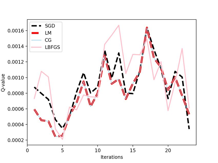
5.3 Effect of Q-Learning
Figure 4 shows the Q-function value being computed in the reinforcement learning experiments. In Cartpole, we see no
effect across all the optimizers, but the flappy bird gives variance across the behaviors. We used the same random seed
7A PREPRINT - M ARCH 2, 2020
values to ensure consistency among all experiments. The figure represents one training episode, covering more than one
trials. The fluctuations represent new trials for the problems. For Flappy Bird, LM provides better convergence than CG
and SGD.But, SGD and CG provides better convergence than LBFGS. This is due to the line search iteration being
limited.
(a) CartPole Episode 1. (b) FlappyBird Episode 1.
Figure 4: Q-value in Deep Reinforcement Experiments.
6 Discussion
6.1 Comparing the Optimizers
Test results show that the second order approaches converge better, but their computational burden is high. Since
conjugate gradient descent is between SGD and second order approaches, it has a calculation advantage over second
order optimizers.
Reinforcement learning experiments show that LM performs better if the problem type is regression. Although it
provides good results for classification purposes, using mean squared error loss function for classification problems
causes computational cost and decrease in performance. Line search algorithm of LBFGS should be chosen properly to
take the advantage of second order derivatives.
6.2 Influence of Training Data Availability
Deep learning approaches require huge training sets, this causes huge memory need and computational costs. Hence,
training step is executed on minibatches. Since training process highly depends on data size, minibatch size should be
chosen carefully. While SGD, CG, and LBFGS use minibatches to calculate gradients, LM requires all samples at a
time and minibatches cannot be used. While it causes high computation burden, it provides better convergence.
6.3 Case for Parallelizing Optimizers
Second order optimizers such as LBFGS and LM provide high rate convergence if computational cost is ignored. In
this study, the line search algorithm of LBFGS was limited to 10 and causes performance drop in LBFGS. On the other
hand, although LM provides good results, its computational cost was too high in comparison to other approaches. Using
distributed line search algorithm may decrease LBFGS computational time while it increases the convergence rate. In
addition to LBFGS, since LM calculates gradient for each sample separately, distributed gradient calculation may make
LM faster.
7 Conclusion
Machine learning projects consist of five key parts: architecture, data, loss function, optimizers, and hyperparameters.
If the one of these are not chosen properly, the algorithm may not perform optimally. One of the challenging steps
of machine learning projects is to determine the loss function and optimizers. They should be in accordance with the
8A PREPRINT - M ARCH 2, 2020
problem type and amount of data. In this study, performances of different optimizers were tested for two different
kinds of machine learning problems on four different datasets with various hyperparameters. Cartpole and Flappy
Bird datasets were chosen from reinforcement learning problem and CIFAR and Mnist datasets were chosen from
classification problems.
While reinforcement learning uses mean squared loss function, classification problems use cross entropy loss function.
The main aim of this study is to investigate the efficiency of optimizers and their appropriate problems. According to the
test results, the importance of line search algorithm used in LBFGS is discovered. Line search algorithms brings tradeoff
between computational cost and accuracy. The advantage of second order algorithms such as Levenberg-Marquardt,
LBFGS is that they provide higher convergence and can represent complex structures. However, high dimensional
feature spaces cause high computational costs for these algorithms.
Other disadvantages of Levenberg-Marquardt is that it is a batch algorithm that mini batches cannot be applied. It
processes each training sample separately to calculate its gradient. It is useful for mean squared error based problems,
classification problems are required to be expressed as regression problems. Conjugate gradient descent approach is
accepted as one and half order algorithm and differs from SGD by its direction selection step. In conjugate gradient,
rather than calculating gradients before the iteration, direction is determined during the iteration. In comparison to the
second order algorithms, it is easier to implement and a little harder than SGD. Results showed that conjugate gradient
descent algorithm provided similar results with SGD.
Finally, second order algorithms provide better convergence under some requirements. While LBFGS requires efficient
line search algorithm to provide remarkable results, LM requires low dimension, compact neural networks and
parameters to be converged. Conjugate gradient descent algorithm is easy to implement and provides good convergence
rates. Since LM calculates gradients per sample separately, if it can be parallelized and computation burden may be
reduced. Moreover, the computational burden of line search algorithm used in LBFGS can be updated with parallel
version of it.
References
[1] Leon Bottou. Stochastic gradient learning in neural networks. In Proceeding in Neural Networks, 1991.
[2] Y. Lecun, L. Bottou, Y. Bengio, and P. Haffner. Gradient-based learning applied to document recognition.
Proceedings of the IEEE, 86(11):2278–2324, Nov 1998.
[3] Quoc V. Le, Jiquan Ngiam, Adam Coates, Abhik Lahiri, Bobby Prochnow, and Andrew Y. Ng. On optimization
methods for deep learning. In Proceedings of the 28th International Conference on International Conference on
Machine Learning, ICML’11, pages 265–272, USA, 2011. Omnipress.
[4] S. Sun, Z. Cao, H. Zhu, and J. Zhao. A survey of optimization methods from a machine learning perspective,
2019.
[5] Fei Wang, Xiaofeng Gao, Jun Ye, and Guihai Chen. Is-asgd: Accelerating asynchronous sgd using importance
sampling. In Proceedings of the 47th International Conference on Parallel Processing, ICPP 2018, New York,
NY, USA, 2018. Association for Computing Machinery.
[6] Jacob Rafati and Roummel F. Marcia. Quasi-newton optimization methods for deep learning applications. arXiv,
2019.
[7] Jacob Rafati and Roummel F. Marcia. Deep reinforcement learning via l-bfgs optimization. arXiv, 2018.
[8] Yang You, Zhao Zhang, Cho-Jui Hsieh, James Demmel, and Kurt Keutzer. Imagenet training in minutes. In
Proceedings of the 47th International Conference on Parallel Processing, ICPP 2018, New York, NY, USA, 2018.
Association for Computing Machinery.
[9] Benjamin Recht, Christopher Re, Stephen Wright, and Feng Niu. Hogwild: A lock-free approach to parallelizing
stochastic gradient descent. In J. Shawe-Taylor, R. S. Zemel, P. L. Bartlett, F. Pereira, and K. Q. Weinberger,
editors, Advances in Neural Information Processing Systems 24, pages 693–701. Curran Associates, Inc., 2011.
[10] Sixin Zhang, Anna E Choromanska, and Yann LeCun. Deep learning with elastic averaging sgd. In C. Cortes,
N. D. Lawrence, D. D. Lee, M. Sugiyama, and R. Garnett, editors, Advances in Neural Information Processing
Systems 28, pages 685–693. Curran Associates, Inc., 2015.
[11] Martín Abadi, Ashish Agarwal, Paul Barham, Eugene Brevdo, Zhifeng Chen, Craig Citro, Greg S. Corrado, Andy
Davis, Jeffrey Dean, Matthieu Devin, Sanjay Ghemawat, Ian Goodfellow, Andrew Harp, Geoffrey Irving, Michael
Isard, Yangqing Jia, Rafal Jozefowicz, Lukasz Kaiser, Manjunath Kudlur, Josh Levenberg, Dandelion Mané, Rajat
Monga, Sherry Moore, Derek Murray, Chris Olah, Mike Schuster, Jonathon Shlens, Benoit Steiner, Ilya Sutskever,
9A PREPRINT - M ARCH 2, 2020
Kunal Talwar, Paul Tucker, Vincent Vanhoucke, Vijay Vasudevan, Fernanda Viégas, Oriol Vinyals, Pete Warden,
Martin Wattenberg, Martin Wicke, Yuan Yu, and Xiaoqiang Zheng. Technical report: Tensorflow: Large-scale
machine learning on heterogeneous systems. https://www.tensorflow.org/, 2015. Software available from
tensorflow.org.
[12] Alexander Sergeev and Mike Del Balso. (technical report)horovod: fast and easy distributed deep learning in
tensorflow, 2018.
[13] Herbert Robbins and Sutton Monro. A stochastic approximation method. Ann. Math. Statist., 22(3):400–407, 09
1951.
[14] Prateek Jain, Sham M. Kakade, Rahul Kidambi, Praneeth Netrapalli, and Aaron Sidford. Parallelizing stochastic
gradient descent for least squares regression: Mini-batching, averaging, and model misspecification. Journal of
Machine Learning Research, 18(223):1–42, 2018.
[15] Minjie Fan. Term Paper: How and Why to Use Stochastic Gradient Descent?, 2017.
[16] Pradeep Ravikumar Aarti Singh. Manual: Conjugate gradient descent. http://www.cs.cmu.edu/~aarti/
Class/10725_Fall17/Lecture_Slides/conjugate_direction_methods.pdf, 2017.
[17] D. F. Shanno. Conditioning of quasi-newton methods for function minimization. Mathematics of Computation,
24(111):647–656, 1970.
[18] Jiang. Hu, Bo. Jiang, Lin. Lin, Zaiwen. Wen, and Ya-xiang. Yuan. Structured quasi-newton methods for
optimization with orthogonality constraints. SIAM Journal on Scientific Computing, 41(4):A2239–A2269, 2019.
[19] Mark Bun. Manual: Applications of the Levenberg-Marquardt Algorithm to the Inverse Problem, 2009.
[20] Rajat Raina, Anand Madhavan, and Andrew Y. Ng. Large-scale deep unsupervised learning using graphics
processors. In Proceedings of the 26th Annual International Conference on Machine Learning, ICML ’09, pages
873–880, New York, NY, USA, 2009. ACM.
[21] Cheng-Tao Chu, Sang Kyun Kim, Yi-An Lin, YuanYuan Yu, Gary Bradski, Andrew Y. Ng, and Kunle Olukotun.
Map-reduce for machine learning on multicore. In Proceedings of the 19th International Conference on Neural
Information Processing Systems, NIPS’06, pages 281–288, Cambridge, MA, USA, 2006. MIT Press.
[22] Rohan Varma. (technical report) picking loss functions - a comparison between mse, cross entropy, and hinge loss.
https://rohanvarma.me/Loss-Functions/, 2018.
[23] Richard S. Sutton and Andrew G. Barto. Reinforcement Learning: An Introduction. A Bradford Book, USA,
2018.
[24] Ankit Choudhary. (technical report) a hands-on introduction to deep q-learning using openai gym in python. https:
//www.analyticsvidhya.com/blog/2019/04/introduction-deep-q-learning-python/, 2019.
[25] Serena Yeung Fei-Fei Li, Justin Johnson. Lecture notes:14 refinforcement learning. http://cs231n.stanford.
edu/slides/2017/cs231n_2017_lecture14.pdf, 2017.
[26] Sebastian Ruder. (technical report) an overview of gradient descent optimization algorithms. https://ruder.
io/optimizing-gradient-descent/, 2016.
[27] Y. H. Dai and Y. Yuan. (technical report) nonlinear conjugate gradient methods. ftp://lsec.cc.ac.cn/pub/
home/dyh/papers/CGoverview.pdf, 2000.
[28] Yu-Hong Dai. (technical report) a perfect example for the bfgs method. ftp://www.cc.ac.cn/pub/dyh/
papers/bfgs-example.pdf, 2013.
[29] Henri P. Gavin. (technical report) the levenberg-marquardt algorithm for nonlinear least squares curve-fitting
problems. http://people.duke.edu/~hpgavin/ce281/lm.pdf, 2013.
[30] Alex Krizhevsky. Learning multiple layers of features from tiny images. Master thesis, University of Toronto, 05
2012.
[31] Cortes LeCun and Burges. (technical report) the mnist database of handwritten digits. http://yann.lecun.
com/exdb/mnist/, 2019.
[32] Naveen Appiah and Sagar Vare. (technical report) playing flappybird with deep reinforcement learning. http:
//cs231n.stanford.edu/reports/2016/pdfs/111_Report.pdf, 2018.
[33] (technical report) getting started with gym. https://gym.openai.com/docs/,year=2019.
10You can also read