A Dissection of Overfitting and Generalization in Continuous Reinforcement Learning
←
→
Page content transcription
If your browser does not render page correctly, please read the page content below
A Dissection of Overfitting and Generalization in
                                                   Continuous Reinforcement Learning

                                                                 Amy Zhang                                Nicolas Ballas
                                                              McGill University                        Facebook AI Research
                                                            Facebook AI Research                         ballasn@fb.com
arXiv:1806.07937v2 [cs.LG] 25 Jun 2018

                                                             amyzhang@fb.com

                                                                                     Joelle Pineau
                                                                                   McGill University
                                                                                 Facebook AI Research
                                                                                   jpineau@fb.com

                                                                                       Abstract

                                                  The risks and perils of overfitting in machine learning are well known. How-
                                                  ever most of the treatment of this, including diagnostic tools and remedies, was
                                                  developed for the supervised learning case. In this work, we aim to offer new
                                                  perspectives on the characterization and prevention of overfitting in deep Rein-
                                                  forcement Learning (RL) methods, with a particular focus on continuous domains.
                                                  We examine several aspects, such as how to define and diagnose overfitting in
                                                  MDPs, and how to reduce risks by injecting sufficient training diversity. This work
                                                  complements recent findings on the brittleness of deep RL methods and offers
                                                  practical observations for RL researchers and practitioners.

                                         1   Introduction
                                         Machine learning is concerned with learning a function from data. That data typically consists of a
                                         mix of pattern and noise. For most supervised learning applications, the data comes from the natural
                                         world, where the pattern may be (near) infinitely complex, and the true noise is not known. Yet
                                         recent studies on generalization in supervised learning have shown that deep neural networks, with
                                         their overparameterization and massive capacity, can lead to memorization of the data, and thus poor
                                         generalization [Zhang et al., 2018, Arpit et al., 2017].
                                         One of the objectives of our work is to explore if similar issues occur in reinforcement learning
                                         (RL). Indeed, recent findings have shown significant brittleness of deep RL methods [Henderson
                                         et al., 2018]. One of the challenges with RL, is that almost all research is done using simulators. By
                                         design, these simulators consist of finite and stationary lines of code, running a deterministic program,
                                         where the only injection of noise is through an initial random seed. In this case, it is not surprising
                                         that (for a fixed random seed), given sufficient data, the RL method will exhaust the noise. In effect,
                                         memorization is inevitable. This is especially prevalent in simple tasks, those with small state spaces,
                                         simple perception, short planning horizon, and deterministic transition functions. This constitutes a
                                         large portion of benchmark domains considered in the field [Brockman et al., 2016, Machado et al.,
                                         2017, Beattie et al., 2016].
                                         In this work we examine conditions under which deep RL achieves generalization vs memorization,
                                         with both model-free and model-based reinforcement learning methods. We investigate the prevalence
                                         of memorization with randomization experiments in both the discrete and continuous action setting,
                                         as well as with value-based and policy-based methods. Through randomized reward experiments,

                                         Preprint. Work in progress.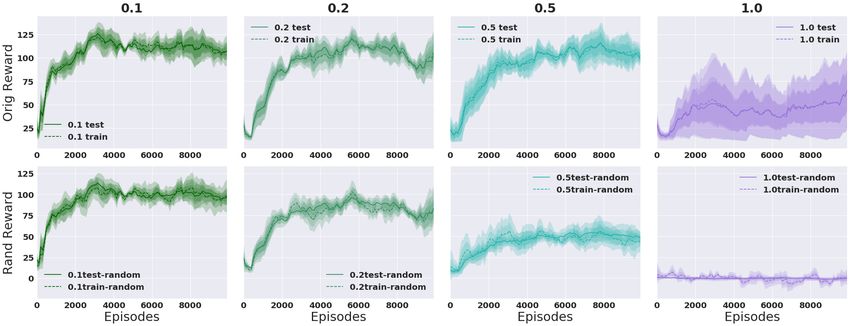
we develop strategies to test memorization. We also propose tests to investigate robustness of the
learned policy specific to the continuous domain, by expanding the initial state distribution and adding
stochastic noise to the observation space.
We first explore classic RL simulated environments such as the Cartpole and Acrobot control tasks in
the Gym toolkit [Brockman et al., 2016] with discrete action space and also look at the continuous
action space setting with MuJoCo Reacher and Thrower environments [Todorov et al., 2012]. As the
goal of RL is eventually to transfer to to the real world, we propose new reinforcement learning tasks
that received observations from natural images and explore generalization in that setting as well.
Our analysis shows that deep RL algorithms can overfit both in standard simulated environment and
when operating on natural images. However, as soon as there is enough training data diversity in the
simulated environment, deep RL generalizes well. It is likely due to the fact that these commonly
used synthetic domains have relatively little noise and spurious patterns. On the other hand, deep
RL algorithms show more prominent overfitting when observing natural data. Those observations
advocate for the development of new benchmarks in order to study more thorough overfitting in deep
RL.

2     Technical Background

Reinforcement Learning. We examine the setting where the environment is a Markov Decision
Process (MDP), represented by a tuple M = (S, A, T, R, S0 , γ), where S is a state space, A an
action space, T (s, a, s0 ) is the state-to-state transition distribution with s, s0 ∈ S, R(s, a) is the
reward function, S0 the initial state distribution, γ ∈ [0, 1) a discount factor [Bellman, 1957]. The
policy π : S → A defines an action selection strategy. Reinforcement learning (RL) is concerned
with finding an optimal policy, denoted π ∗ : S → A, that maximizes the expected sum of rewards.
Value function estimation. The value function defines the expected sum of rewards over the
                                                              PT
trajectory t = 0...T while following policy π: V π (s) = E[ t=0 γrt |s0 = s]. The state-action Q-
function
       Pis similarly defined and can be recursively estimated from Bellman’s equation: Qπ (st , at ) =
rt + γ s0 ∈S T (s, a, s )maxa0 ∈A Q(s0 , a0 ).
                        0

In the absence of a known transition model T (), the Q-function can be estimated from a batch of
data using fitted Q-iteration, which learns an approximate function Q̂(·, θ), parameterized by θ,
                                               2
minimizing the loss: L(θ) = Q̂(st , at , θ) − Yt , where Yt = rt + γ maxa Q(st+1 , a, θ).
Deep RL. The Deep Q-Network (DQN) extends fitted Q-iteration by using a (potentially large) neural
network for the Q-function [Mnih et al., 2015]. Several additional steps are helpful in stabilizing
learning, including using a target network from a previous iteration, applying L1-smoothing of the
loss, incorporating experience replay [Mnih et al., 2015], and correcting with Double DQN [van
Hasselt et al., 2015]. This class of approach is suitable for continuous state, discrete action MDPs.
Policy-based Methods. In the case of continuous action domains, policy-based methods are
typically used. Here we directly estimate a parameterized form of the optimal policy πθ (s),
where in deep RL πθ (s) takes the form of a neural network. This network takes as input the
state st , outputs
                a distribution over possible
                                                  actions at , and is trained with a loss of the form:
LPG (θ) = Êt log πθ (at |st )Âπ (st , at ) . Proximal Policy Optimization (PPO) [Schulman et al.,
2017] is a popular variant of policy gradient methods that incorporates constraints on the policy
change, as well as mini-batches and multiple epochs of learning between each query of the environ-
ment.

3     Perspectives on generalization and overfitting

3.1   Generalization in Supervised Learning

In Supervised Learning (SL), we assume an unknown data distribution D from which we draw
i.i.d samples Xtrain with ground truth labels Ytrain where y ∈ Y are extracted from a target concept
y = c(x). The goal is to learn a function f that learns the mapping from Xtrain to Ytrain . Given a loss
function l(f (x), y), the generalization error EG is defined as the difference in true and expected error.

                                                    2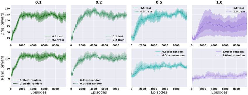
N
                                                               1 X
                               EG = Ex,y∼D [l(f (x), y] −            l(f (xtr,i ), ytr,i )                        (1)
                                                               N i=1
In practice, however, we do not have access to underlying joint probability distribution p(x, y).
Instead, we compute a proxy empirical error using a withheld test set (Xtest , Ytest ) drawn from the
same distribution as (Xtrain , Ytrain ). This gives us the following formula for generalization error:
                                       M                             N
                                    1 X                           1 X
                            EG =          l(f (xte,i ), yte,i ) −       l(f (xtr,i ), ytr,i )                     (2)
                                    M i=1                         N i=1
where N = |Xtrain |, M = |Xtest |, (xtr,i , ytr,i ) ∈ (Xtrain , Ytrain ), and (xte,i , yte,i ) ∈ (Xtest , Ytest ).
Overfitting is defined as poor generalization behavior, or large EG .
Recent work [Zhang et al., 2016] explores the issue of generalization performance in the supervised
setting, showing that deep neural networks are capable of memorizing random data, thus exhibiting
extreme overfitting.
An interesting question is whether analogous concepts of generalization, memorization and overfitting
arise in the reinforcement learning framework.

3.2        Generalization and Memorization in Reinforcement Learning

We focus on characterizing and diagnosing overfitting in deep Reinforcement Learning (RL) methods,
with a specific focus on continuous domains. The continuous state space case is particularly interesting
with deep reinforcement learning because it is a setting where we expect function approximation (and
particularly, a function represented by a deep neural network) to perform well. The continuous state
setting is also interesting because we cannot feasibly explore all possible initial states during training
time, thus we suppose that generalization is necessary to solve the task1 .
Considering the fact that almost all research in RL is done using simulators, to further examine
generalization and overfitting it is necessary to consider cases where (1) the dataset is much smaller
than the complexity of the simulator, (2) the random seed is varied to create noise (thus inducing
variance in the trajectories due to different initial states or transitions), or alternately (3) the simulator
itself is drawn from a random distribution (e.g. by varying the initial state distribution, or transition
function, or reward function). We investigate all three cases in experiments below. Cases 1 & 2
correspond to within-task generalization; case 3 corresponds to out-of-task (or transfer) generalization.
In the within-task case, generalization is achieved when a policy trained on an initial set of training
trajectories is shown to perform well on a set of test trajectories generated by the same simulator. In
the out-of-task case, generalization is achieved when a policy trained on one setting of the simulator
performs well on another setting of the simulator.
As exposed above, the only source of noise when doing RL in a simulated environment is through the
random seed. Thus, as also proposed in Zhang et al. [2018], the only way to achieve a separation
between training and testing sets is by separation of random seeds. Define S0,train to be the
trajectories generated by the set of training seeds, and S0,test to be the set of trajectories generated by
the testing seed.
We can now define generalization in RL:
                           N T                                      M T
                        1 XX                                     1 XX
             EG,RL =              R(st , πθ (st )|s0 = str,i ) −           R(st , πθ (st )|s0 = ste,i ),          (3)
                        N i=1 t=1                                M i=1 t=1
where N is the number of training seeds, M is the number of test seeds, str,i ∈ S0,train , ste,i ∈
S0,test , T is the length of each episode, and πθ is our parameterized policy in the policy-based
method case, and πθ = arg maxa Qθ (s, a) in the value-based method case. In practice, for all of our
experiments, we fix the number of test seeds to be M = 100.
In addition to simulated environments, we also propose new tasks where observations are grounded
in natural data. We investigate deep-RL generalization behaviors on tasks where noise comes from a
natural source in that setting.
      1
          Our work was done concurrently with Zhang et al. [2018], which focuses on the discrete state setting.

                                                           3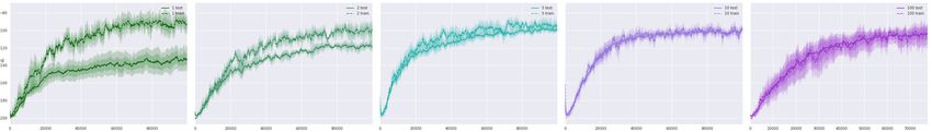
4         Overfitting and memorization in the within-task case

In this section we perform a series of empirical demonstrations to illustrate the various incarnations
of overfitting in RL. Several details of the experimental setup, including domain specification, deep
learning architecture and training regime are included in the appendix. They are not necessary to
understand the main findings, but may be useful for reproducing the work.

4.1       On the effect of the number of training random seeds

Consider the case where we fix the number test seeds to M = 100 and vary the number of training
seeds. We track the difference in performance on the initial state drawn from the set of train seeds vs.
the set of test look at the difference in performance.
Discrete Action Space. Experiments with discrete action spaces use a Double DQN architecture.
Full implementation details are in the appendix and code will be released. We first consider the
popular Acrobot task [Sutton, 1996]. We look at 2 versions of this domain: a first where the state
space is defined over the 6-dimensional joint position & velocity space, and a second where the
state is described in pixel space from a visual representation of the domain. In the pixel case we
concatenate multiple consecutive screens to allow velocity estimation, and thus circumvent partial
observability. Figure 1 shows overfitting in both representations, for smaller number of training
seeds2 . When the number of training seeds gets to be around 10, there is sufficient diversity in training
data to generalize well given the simplicity of the environment.

Figure 1: The 6-dim Acrobot (left) and Pixel Acrobot (right), varying number of train seeds from 1 to
100, with γ = 0.99. Averaged over 5 runs. Trained for 10K episodes (6-dim) and 100K episodes
(Pixel).
Next we consider the ubiquitous Cartpole domain. Again, we investigate using the standard 4-
dimensional state space (position and velocity of the cart, plus angle and angular velocity of the pole).
We also consider Pixel Cartpole, which uses a visual representation of the task. For this domain,
looking at Fig. 2, we do not see any overfitting with the lower dimensional representation. However
overfitting is clearly seen in the Pixel Cartpole case.
In both domains, by controlling the number of seeds drawn from the initial state distribution, we can
effectively control the amount of overfitting occurring. And the number of seeds necessary is quite
small, though this is likely due to the fact that these simulated domains have relatively little noise.
Continuous Action Space. Next we consider overfitting in continuous action spaces using PPO
[Schulman et al., 2017] to train the RL on domains from the MuJoCo suite [Todorov et al., 2012] as
implemented in the Gym simulator [Brockman et al., 2016]. We consider the 11-dim state space for
Reacher and 23-dim state space Thrower. Reacher consists of two links with the task of reaching a
goal point, while Thrower consists of an agent attempting to throw a ball into a goal box. In both
environments, the goal is initialized randomly for each seed (training and test).
Figure 3 shows that the RL achieves good generalization in the Reacher, but suffers from overfitting
in the Thrower with small numbers of training seeds. However at 5 training seeds and more the policy
learns to generalize to unseen goal locations (as evaluated over 100 test goals).
      2
     Note that with a single training seed, the initial state drawn is always the same. However, the number of
states seen during training is still |A||e| where |e| is the length of episode e when using a discrete action space.

                                                         4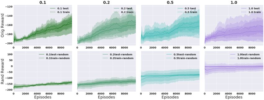
Figure 2: 4-dim Cartpole (left), Pixel Cartpole (right), varying number of train seeds with γ = 0.995.
Averaged over 5 runs. 10K episodes.

Figure 3: Reacher (top left), Thrower (top center), ThrowerMulti (top right), varying number of train
seeds with γ = 0.99. Averaged over 5 runs. Trained with 10M steps each. Expanded view of reward
for ThrowerMulti (bottom).

In addition, we consider a modified Thrower environment (ThrowerMulti): instead of a single goal
box, there are now 5 goal boxes placed in random locations. The state now includes a goal id which
designates which goal is the correct one – reaching the others provides no reward. The goal of this
modification is to check whether the number of seeds necessary grows with the task complexity.
Indeed, as shown in Fig. 3, we need a larger number of training seeds to achieve good performance.
With the addition of a single free variable, ThrowerMulti now exhibits overfitting even in the 100 seed
case. We also clearly see in the 1 seed case that the policy first learns a simple policy that performs
slightly better for evaluation, but over time overfits to the train case, causing evaluation performance
to drop. The performance on the test seeds for ThrowerMulti is also very high variance compared to
that on training seeds and compared to that on the original Thrower domain.
Natural Images. We also evaluate for overfitting in natural images with a pixel-by-pixel reinforce-
ment learning task. We use MNIST LeCun and Cortes [2010] and CIFAR10 Krizhevsky et al.,
creating an exploration task where an agent is always spawned in the center of a masked image. The
state consists of the agent’s position and the 28x28 masked image. At each time step, the agent can
move left, right, up, or down, which reveals a square window w of the image. After each time step
the agent classifies what the masked image is, and episode ends with reward 1 when it classifies
the image successfully. Otherwise it fails after a maximum 100 time steps. We compare against
a baseline where it is given the entire image to classify at the end of each episode. MNIST and
CIFAR10 results are given in Figure 4.
With natural images, we see even in the 10k training seed case (trained on 10k images), there is a
generalization gap. If we compare this with the baseline we see more overfitting effect, since there
are now multiple possible partially masked images that correspond to a single image. We see similar
effects in CIFAR10 results in Figure 4.

                                                   5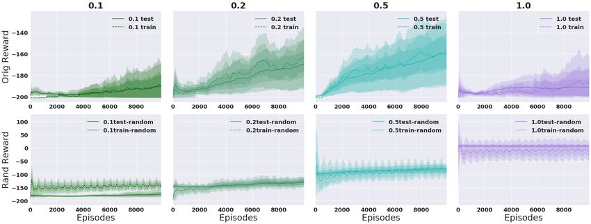
Figure 4: Generalization gap for MNIST (top left) and MNIST baseline (top center) where number of
seeds corresponds to number of unique images. Total reward given for MNIST (bottom). Window
size w = 5. CIFAR10 result (top right) with w = 10.
4.2 On memorization in RL: a randomized reward test
The phenomenon of memorization in supervised learning is examined by assigning random labels
to training examples [Zhang et al., 2018, Arpit et al., 2017]. This does not extend directly to the
RL setting. Instead, we propose to examine memorization by injecting randomness into the reward
function. In most continuous domains, the reward varies relatively smoothly over the state space, or
at least there are few discontinuities (e.g. when reaching a goal area). By randomizing the reward
function, we can examine whether RL models exhibit memorization and learn spurious patterns that
will not generalize. When there are few perturbations to the reward, or there are many training seeds,
the policy should still able to learn the given reward signal. However, when the reward function
becomes more erratic, it should be more difficult for the policy to train and to generalize well.
To create randomized reward functions, we bin the state space into k equal bins. For each bin, we
uniformly at random choose a reward multiplier β between [−1, 1]. These multipliers are deterministic
– they are consistent for a specific seed, but different across different initial states s0 . We control
the amount of randomness injected into the environment with a parameter prand , where prand is the
probability of each bin having its reward signal modified by the multiplier.
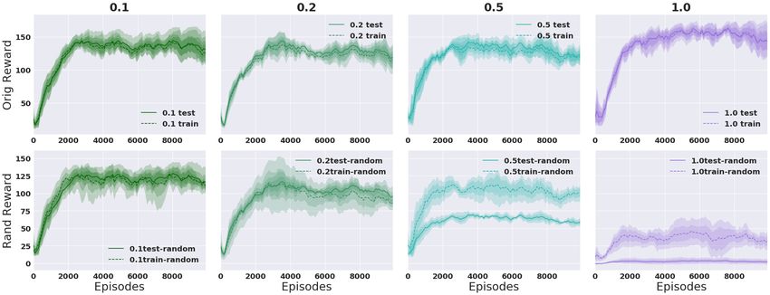
Discrete Action Space. Figure 5 shows k = 3 bins for Cartpole with a single train seed (top)
and 100 train seeds (bottom). The model is trained on random reward with train seeds, with
prand ∈ [0.1, 0.2, 0.5, 1]. In this case we see performance start to drop off as p increases. For low prand ,
the model is able to effectively ignore the noise. In the 1 seed case we see the model successfully
learn the random reward, especially noticeable in the prand = 0.5 and prand = 1.0 columns. However,
the model does not have the capacity to memorize all the random rewards even in the 100 seed case,
and so it only learns the true reward signal up until performance collapses when prand = 1.0, where
there is no true reward signal left and the random reward is too complex to learn3 . Additional results
for the Acrobot domain can be found in Appendix B.2.
Continuous Action Space. Figure 6 shows results for Thrower with randomized rewards. Again we
see that it is easy to memorize the random reward in the 1 seed case, but much harder in the 100
seed case, and so it instead learns to concentrate on the true reward signal. We observe much larger
variance in the single training seed case. Similar results for Reacher can be found in Appendix B.3.
Natural Images. Figure 7 shows results for MNIST with randomized labels. As p increases we see
inability to generalize to the test set, but that we can still achieve perfect memorization on the training
set. We had to increase the capacity of the model and use a ResNet-18 He et al. [2015] as backbone
to achieve perfect memorization on the 10k train set.
3
Note that in the Cartpole environment any policy that can find positive reward (even random reward) and
optimize for it will also perform well on the original task – the family of policies for the original environment is
a superset of policies for any reward function with a positive signal that incentivizes prolonging the episode.
6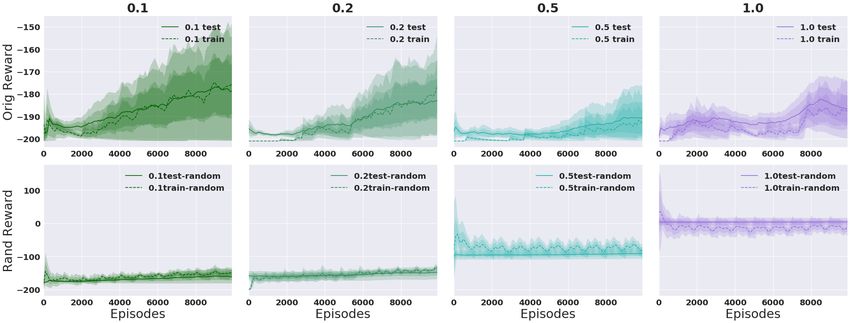
Figure 5: k = 3. Full experiments on randomizing reward on 4-dim Cartpole: Varying prand (cols)
with γ = 0.995 and 1 training seed (top), 100 training seeds (bottom). Averaged over 5 runs. Models
are trained on the random reward and evaluated on the original reward.

Figure 6: Thrower, varying prand of each bin randomized with k = 3 and γ = 0.99. Averaged over 5
runs. 1 seed (top), 100 seeds (bottom).*
*
 Reward values are not directly comparable across columns because the percentage of bins modified by the
random multiplier changes the average reward obtained by a random policy.

Figure 7: Train and test performance with increasing p from left to right on MNIST 10k. Window
size w = 5.

                                                   7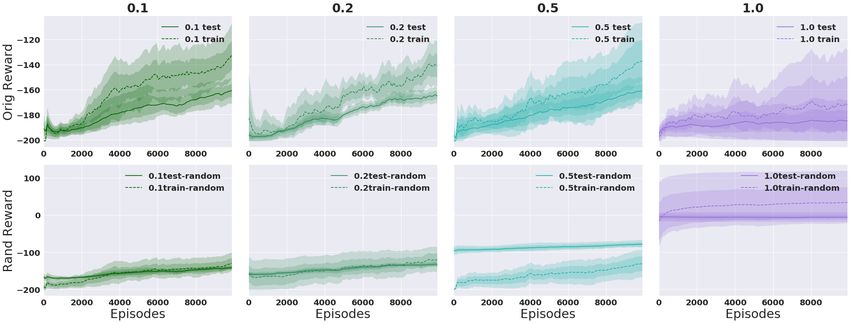
5    The out-of-task case for generalization in RL
Moving beyond the case where noise is induced only via the random seed, we now consider cases
where it is valuable to generalize over possible distributional shifts between training and evaluation
conditions. This is closer to the case considered in previous work on overfitting in RL [Whiteson
et al., 2011, Zhang et al., 2018], and in the broadest sense extends to notions of transfer [Taylor and
Stone, 2009] and zero/few-shot learning [Oh et al., 2017].
We consider the cases where the state and action sets are the same, but noise may induce changes in
transition dynamics, reward function, or initial state distribution. There is evidence (in the discrete
state setting) that if the number of tasks you train on is not varied enough, the model tends to
memorize the specific environments and learn them explicitly [Zhang et al., 2018]. When trained on
enough environments, we expect generalization to allow the RL agent to navigate efficiently on new
test environments drawn from the same distribution.
Recall that our goal is not to study transfer broadly, but to examine notions of overfitting and
generalization in realistic conditions. Thus we consider two mechanisms for injecting noise into
the domain. First we consider an expansion of the initial state distribution, which we implement
by applying a multiplier to the initial state chosen. In the MuJoCo domains, the state is initialized
uniformly at random from a given range for each dimension. We want to evaluate a specific shift
where we train with initial state distribution Strain,0 and evaluate with different initial state distribution
Stest,0 . We investigate the setting where Stest,0 is a strict superset of Strain,0 , but this evaluation can
also occur in sets with no overlap. In practice, we expand this initial state s0 with a multiplier m
to get new initial state s00 = ms0 . We vary the magnitude of the multiplier m to see the effect of
increasing the noise. The results in Table 1 confirm that the generalization improves significantly
with more training seeds, but is made more difficult when there is increased noise in the simulation
distribution.
                        # OF T RAINING                 I NITIAL    S TATE     M ULTIPLIER
    E NVIRONMENT            S EEDS          m=1         m=5        m = 10       m = 20         m = 100
                               1           -101.09      -95.49     -97.24       -101.13        -110.31
    T HROWER                   2            -74.59      -77.86     -78.38        -78.37         -84.84
                               5            -52.77      -53.58     -54.67        -53.93         -64.51
                              10            -53.67      -53.71     -54.10        -56.69         -70.66
                             100            -49.68      -49.24     -51.41        -50.32         -58.85
Table 1: Out-of-task generalization on Thrower, reporting the estimated value averaged over 100 test
seeds. Columns indicate the multiplier on the initial state.

Second, we evaluate policy robustness by adding Gaussian noise n ∼ N (0, σ 2 ) directly to the
observation space. We add zero-mean Gaussian noise with variance σ 2 to each observed state at
evaluation, and measure robustness of the policy as we increase σ 2 . The results in Table 2 follow a
similar trend as those in Table 1.
                               # OF T RAINING                 VARIANCE OF N OISE
            E NVIRONMENT           S EEDS          σ 2 = 0.        σ 2 = 0.1           σ 2 = 0.2
                                      1             -99.1           -106.0              -114.8
            T HROWER                  2             -74.4            -84.8              -100.0
                                      5             -52.3            -69.0              -106.3
                                     10             -52.7            -72.6              -103.0
                                    100             -49.8            -64.2               -93.7
Table 2: Transfer experiments on Thrower. Columns indicate the variance σ 2 of the Gaussian noise
added to the observation space.

6    The effect of model-based RL
Several claims have been made about the fact that model-based RL improves robustness of results.
We therefore finish our investigation by looking into the generalization abilities of model-based RL
methods (Fig. 8). We consider a Double DQN architecture with an additional two heads that output a
prediction of next state and reward (in addition to Q-value). We consider the same modification to
the critic to transfer PPO into a model-based approach.

                                                      8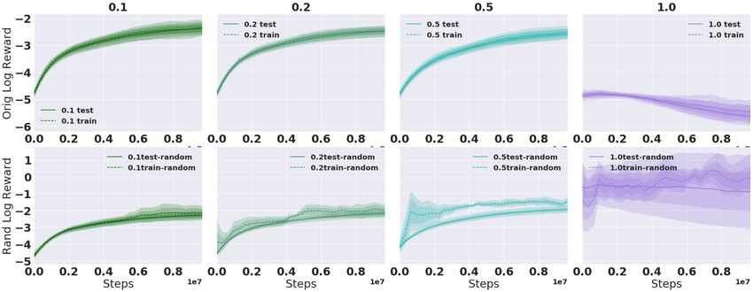
Figure 8: Model-based Reacher (left), and Thrower (right). Varying number of train seeds from 1 to
100 with γ = 0.99. Averaged over 5 runs.
Results suggest that explicitly learning the dynamics model compounds existing bias in the data
in the limited training seed regime. We invite the reader to examine Figure 8 and compare with
the model-free results in Figure 3. We see that Reacher now exhibits generalization error in the
model-based case where it did not in the model-free case, and the generalization gap has increased
for Thrower.

7   Related Work

While not as prevalent as in the SL case, there has been some work exploring evaluation of generaliza-
tion and overfitting in RL. Rajeswaran et al. [2017] show with linear and RBF parameterizations that
they can achieve surprisingly good generalization compared to more elaborate parameterizations, and
thus call for simpler linear models for better generalization. However, this is unrealistic for tasks with
highly complex dynamics or nonlinear mapping between the state and value space. Francois-Lavet
et al. [2017] also looks at overfitting in the batch reinforcement learning case in POMDPs (Partially
Observable Markov Decision Processes), specifically exploring the bias-variance tradeoff in the
limited data scenario. They are limited to the batch setting in order to control the number of samples,
but we look at the limited data setting by controlling the number of seeds, and therefore can still
analyze online approaches.
Murphy [2005] analyzes generalization error for Q-learning with function approximation in the batch
case. They define generalization error as the average difference in value when using the optimal policy
as compared to using the greedy policy based on the learned value function. This requires knowing
the optimal policy, which is infeasible in many environments. Ponsen et al. [2010] is a survey of
abstraction and generalization in RL and also touches upon the notion of transfer as generalization.
Concurrent work [Zhang et al., 2018] shows memorization in reinforcement learning in the discrete
domain with gridworld experiments. Our analysis focuses on continuous domains with effectively
infinite number of states, which can be more complex and closer to many real world settings.

8   Conclusion

Currently, much RL work is still being done in simulation, with the goal of eventually transferring
methods and policies to the real world. Of course we know that simulated environments lack the di-
versity – complex signal, natural noise, nonstationary stochasticity – of real world environments. Our
natural image experiments show the discrepancy in number of seeds required for true generalization
compared to the simulation environments. But until we drastically improve the sample complexity of
RL methods, developing and testing in simulation will remain common. Simulated environments
also continue to be a necessary tool as a controllable benchmark to compare methods, since it is not
possible to “share the real world.”
Given this state of affairs, we have conducted a thorough investigation into the pitfalls of overfitting
in continuous RL domains. We present a methodology for detecting overfitting, as well as eval-
uation metrics for within-task and out-of-task generalization. Especially in robotics tasks where
it is infeasible to train on the same distribution as evaluation, our work shows the discrepancy in
performance that we can expect to see in transfer scenarios. This methodology also decouples

                                                    9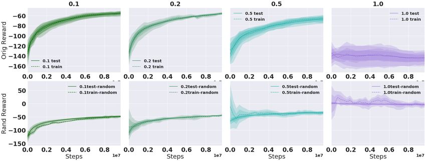
evaluation of generalization from sample complexity for online methods. As deep reinforcement
learning gains more traction and popularity, and as we increase the capacity of our models, we need
rigorous methodologies and agreed upon protocols to define, detect, and combat overfitting. Our
work contains several simple useful lessons that RL researchers and practitioners can incorporate to
improve the quality and robustness of their models and methods.

References
D. Arpit, S. Jastrzebski, N. Ballas, D. Krueger, E. Bengio, Kanwal M.S., T. Maharaj, A. Fischer,
  A. Courville, Y. Bengio, and S. Lacoste-Julien. A closer look at memorization in deep networks.
  In ICML, 2017.
Charles Beattie, Joel Z. Leibo, Denis Teplyashin, Tom Ward, Marcus Wainwright, Heinrich Küttler,
  Andrew Lefrancq, Simon Green, Víctor Valdés, Amir Sadik, Julian Schrittwieser, Keith Anderson,
  Sarah York, Max Cant, Adam Cain, Adrian Bolton, Stephen Gaffney, Helen King, Demis Hassabis,
  Shane Legg, and Stig Petersen. Deepmind lab. CoRR, abs/1612.03801, 2016.
R. Bellman. A Markovian Decision Process. Journal of Mathematics and Mechanics, 1957.
Greg Brockman, Vicki Cheung, Ludwig Pettersson, Jonas Schneider, John Schulman, Jie Tang, and
  Wojciech Zaremba. Openai gym, 2016.
V. Francois-Lavet, D. Ernst, and R. Fonteneau. On overfitting and asymptotic bias in batch reinforce-
   ment learning with partial observability. ArXiv e-prints, September 2017.
Kaiming He, Xiangyu Zhang, Shaoqing Ren, and Jian Sun. Deep residual learning for image
  recognition. CoRR, abs/1512.03385, 2015.
P. Henderson, R. Islam, and Pineau J. Precup D. Meger D. Bachman, P. Deep reinforcement learning
   that matters. In AAAI, 2018.
Diederik P. Kingma and Jimmy Ba.          Adam: A method for stochastic optimization.           CoRR,
  abs/1412.6980, 2014.
Alex Krizhevsky, Vinod Nair, and Geoffrey Hinton. Cifar-10 (canadian institute for advanced
  research). URL http://www.cs.toronto.edu/~kriz/cifar.html.
Yann LeCun and Corinna Cortes. MNIST handwritten digit database. 2010. URL http://yann.
  lecun.com/exdb/mnist/.
Marlos C. Machado, Marc G. Bellemare, Erik Talvitie, Joel Veness, Matthew J. Hausknecht, and
 Michael Bowling. Revisiting the arcade learning environment: Evaluation protocols and open
 problems for general agents. CoRR, abs/1709.06009, 2017.
Volodymyr Mnih, Koray Kavukcuoglu, David Silver, Andrei A. Rusu, Joel Veness, Marc G. Belle-
  mare, Alex Graves, Martin Riedmiller, Andreas K. Fidjeland, Georg Ostrovski, Stig Petersen,
  Charles Beattie, Amir Sadik, Ioannis Antonoglou, Helen King, Dharshan Kumaran, Daan Wierstra,
  Shane Legg, and Demis Hassabis. Human-level control through deep reinforcement learning.
  Nature, 518(7540):529–533, 02 2015. URL http://dx.doi.org/10.1038/nature14236.
Susan A. Murphy. A generalization error for q-learning. J. Mach. Learn. Res., 6:1073–1097,
  December 2005. ISSN 1532-4435. URL http://dl.acm.org/citation.cfm?id=1046920.
  1088709.
J. Oh, S. Singh, H. Lee, and P. Kohli. Zero-shot task generalization with multi-task deep reinforcement
   learning. In ICML, 2017.
Marc Ponsen, Matthew E. Taylor, and Karl Tuyls. Abstraction and generalization in reinforcement
 learning: A summary and framework. In Matthew E. Taylor and Karl Tuyls, editors, Adaptive
 and Learning Agents, pages 1–32, Berlin, Heidelberg, 2010. Springer Berlin Heidelberg. ISBN
 978-3-642-11814-2.
A. Rajeswaran, K. Lowrey, E. Todorov, and S. Kakade. Towards Generalization and Simplicity in
  Continuous Control. ArXiv e-prints, March 2017.

                                                  10
John Schulman, Filip Wolski, Prafulla Dhariwal, Alec Radford, and Oleg Klimov. Proximal policy
optimization algorithms. CoRR, abs/1707.06347, 2017.
Richard S. Sutton. Generalization in reinforcement learning: Successful examples using sparse coarse
coding. In Advances in Neural Information Processing Systems 8, pages 1038–1044. MIT Press,
1996.
M. Taylor and P. Stone. Transfer learning for reinforcement learning domains: A survey. JMLR,
2009.
Emanuel Todorov, Tom Erez, and Yuval Tassa. Mujoco: A physics engine for model-based control. In
IROS, pages 5026–5033. IEEE, 2012. ISBN 978-1-4673-1737-5. URL http://dblp.uni-trier.
de/db/conf/iros/iros2012.html#TodorovET12.
Hado van Hasselt, Arthur Guez, and David Silver. Deep reinforcement learning with double q-
learning. CoRR, abs/1509.06461, 2015.
S. Whiteson, B. Tanner, M. E. Taylor, and P. Stone. Protecting against evaluation overfitting in
empirical reinforcement learning. In 2011 IEEE Symposium on Adaptive Dynamic Programming
and Reinforcement Learning (ADPRL), pages 120–127, April 2011. doi: 10.1109/ADPRL.2011.
5967363.
C. Zhang, S. Bengio, M. Hardt, B. Recht, and O. Vinyals. Understanding deep learning requires
rethinking generalization. ArXiv e-prints, November 2016.
C. Zhang, O. Vinyals, R. Munos, and S. Bengio. A Study on Overfitting in Deep Reinforcement
Learning. ArXiv e-prints, April 2018.
11A Model Specifications and Hyperparameters
Convolutional head for pixel space consists of 3 convolutional layers with middle dim 512 and ReLU
nonlinearities.
A.1 Double DQN
• lr: 3e-3 for low-dim, 3e-4 for pixel
• target update interval: 1000
• replay memory: 1M for low-dim, 100K for pixel
• Architecture: 3-layer MLP with middle dim 512
• γ: 0.995 for Cartpole, 0.99 for Acrobot
A.2 PPO
• lr: 3e-4
• PPO epochs: 10
• Number of steps between updates: 2048
• γ: 0.99
• Batch size: 32
• Architecture: 3-layer MLP with middle dim 512
Used Adam Kingma and Ba [2014] as optimizer.
B Environments
B.1 Cartpole
B.1.1 Random Reward
The random reward is binning the angle θ of the pole. Each bin has a probability p of having a
randomized reward with its own random multiplier between -1 and 1.
4-Dim Cartpole Full randomized reward experiments varying the number of training seeds, number
of bins b, and randomization probability p.
Figure 9 shows random rewards on Cartpole with k = 3 bins and varying the probability p ∈
[0.1, 0.2, 0.5, 1], with evaluation done with the original reward. This experiment is done on the
original 4-dimensional state space for Cartpole. The original reward function of Cartpole returns a
reward of 1 at every step, so we see that we still get enough positive reward signal for the original
Cartpole to perform quite well even when all k bins are assigned a random multiplier.
Number of episodes: 10K
Pixel Cartpole Full randomized reward experiments varying the number of training seeds, number
of bins b, and randomization probability p.
Number of episodes: 10K Replay memory: 100K (s, a, r, s0 ) tuples Learning rate: 3e-4
B.2 Acrobot
Acrobot is a 2-link pendulum with only the second joint actuated. It is instantiated with both links
pointing downwards. The goal is to swing the end-effector at a height at least the length of one link
above the base.
The state consists of the sin() and cos() of the two rotational joint angles θ1 , θ2 and the joint angular
velocities.
[cos(θ1 ) sin(θ1 ) cos(θ2 ) sin(θ2 )θ̇1 θ̇2 ] (4)
12Figure 9: b = 3. Full experiments on randomizing reward on 4-dim Cartpole: Varying p (cols) with
γ = 0.995 and varying 1, 10, 100 training seeds (rows). Averaged over 5 runs.
For the first link, an angle of 0 corresponds to the link pointing downwards. The angle of the second
link is relative to the angle of the first link. An angle of 0 corresponds to having the same angle
between the two links. The action is either applying +1, 0 or -1 torque on the joint between the two
pendulum links.
Number of episodes: 10K
B.2.1 Random Reward
We bin θ0 , the angle of the first link of the pendulum.
13Figure 10: Model-based. Pixel Cartpole. Two states, varying number of train seeds with γ = 0.99.
Averaged over 5 runs.
B.3 Reacher
Reward on a log scale. (negated, log, then negated again)
Number of frames: 10M
B.3.1 Random Reward
For Reacher, we randomize reward by binning θ, the angle of the first link.
B.4 Thrower
Number of frames: 100M
B.4.1 Random Reward
We bin the first dimension of the observation space.
C Transfer
E NVIRONMENT S EED σ 2 = 0. σ 2 = 0.0001 σ 2 = 0.0005 σ 2 = 0.001 σ 2 = 0.002
1 89.7 90.3 75.5 47.4 26.7
C ARTPOLE 2 131.3 131.3 112.9 69.5 35.4
5 105.7 102.7 66.6 39.1 19.2
10 145.5 144.1 122.8 101.5 78.8
100 122.4 119.9 99.7 66.8 35.8
σ 2 = 0. σ 2 = 0.1 σ 2 = 0.2 σ 2 = 0.3 σ 2 = 0.4
1 19.4 19.2 18.8 18.9 19.6
P IXEL C ARTPOLE 2 20.3 18.2 17.9 18.3 19.1
5 22.5 20.0 20.2 20.3 20.4
10 16.4 19.8 20.6 20.6 20.2
100 21.7 17.4 17.3 17.4 18.0
σ 2 = 0. σ 2 = 0.001 σ 2 = 0.002 σ 2 = 0.003 σ 2 = 0.004
1 31.4 34.2 17.9 16.3 15.2
P IXEL C ARTPOLE 2 29.5 31.5 17.2 17.2 16.5
(M ODEL BASED ) 5 35.2 38.2 20.0 21.7 21.3
10 31.1 35.7 19.7 18.6 18.4
100 25.2 30.5 18.9 18.5 19.0
Table 3: Transfer experiments on Cartpole and Pixel Cartpole for model-free and model-based.
Columns indicate the variance σ 2 of the Gaussian noise added to the observation space. Note the
difference in σ 2 of noise for all three settings.
14E NVIRONMENT S EED σ 2 = 0. σ 2 = 0.01 σ 2 = 0.05 σ 2 = 0.1 σ 2 = 0.2
ACROBOT 1 -130.4 -132.1 -156.8 -185.7 -198.6
2 -118.7 -120.0 -170.8 -193.1 -199.0
5 -95.0 -98.8 -137.2 -174.5 -193.1
10 -100.6 -100.4 -134.9 -172.6 -196.2
100 -107.5 -111.9 -155.1 -182.8 -196.8
σ 2 = 0. σ 2 = 0.001 σ 2 = 0.002 σ 2 = 0.003 σ 2 = 0.004
1 -128.1 -129.6 -198.9 -199.9 -200.0
P IXEL ACROBOT 2 -109.8 -109.2 -199.9 -200.7 -200.7
5 -87.2 -89.0 -200.2 -199.8 -200.2
10 -96.8 -97.6 -199.9 -199.6 -200.2
100 -83.6 -84.7 -200.3 -199.9 -200.7
Table 4: Transfer experiments on Acrobot. Columns indicate the variance σ 2 of the Gaussian noise
added to the observation space.
E NVIRONMENT S EED σ 2 = 0. σ 2 = 0.1 σ 2 = 0.2 σ 2 = 0.5 σ 2 = 1.
R EACHER 1 -11.3 -11.8 -12.1 -13.5 -15.2
2 -27.2 -27.1 -26.1 -24. -24.6
5 -13.8 -14.9 -15.5 -16.7 -18.8
10 -11.8 -11.7 -12.1 -13.8 -13.7
100 -11.4 -11.4 -11.7 -12.7 -14.3
Table 5: Transfer experiments on Reacher. Columns indicate the variance σ 2 of the Gaussian noise
added to the observation space.
15Figure 11: b = 3. Full experiments on randomizing reward on Acrobot: Varying p (cols) with
γ = 0.99 and varying 1, 2, 5 and 10 training seeds (rows). Averaged over 5 runs. 100K episodes.
16Figure 12: Reward for Acrobot varying number of training seeds. Averaged over 5 runs.
Figure 13: b = 3. Full experiments on randomizing reward on Reacher: Varying p (cols) with
γ = 0.99 and 1 and 100 training seed (rows). Averaged over 5 runs.
17Figure 14: b = 3. Full experiments on randomizing reward on model-based Reacher: Varying p (cols)
with γ = 0.99 and 1 and 100 training seeds (rows). Averaged over 5 runs.
18Figure 15: k = 3. Full experiments on randomizing reward on Thrower: Varying p (cols) with
γ = 0.99 and 1 and 100 training seeds. Averaged over 5 runs.
19Figure 16: b = 3. Full experiments on randomizing reward on model-based Thrower: Varying p
(cols) with γ = 0.99 and 1 and 100 training seeds (rows). Averaged over 5 runs.
20You can also read