BOUNDED MYOPIC ADVERSARIES FOR DEEP REINFORCEMENT LEARNING AGENTS
←
→
Page content transcription
If your browser does not render page correctly, please read the page content below
Under review as a conference paper at ICLR 2021

B OUNDED M YOPIC A DVERSARIES FOR
D EEP R EINFORCEMENT L EARNING AGENTS
 Anonymous authors
 Paper under double-blind review

                                            A BSTRACT

         Adversarial attacks against deep neural networks have been widely studied. Ad-
         versarial examples for deep reinforcement learning (DeepRL) have significant
         security implications, due to the deployment of these algorithms in many applica-
         tion domains. In this work we formalize an optimal myopic adversary for deep
         reinforcement learning agents. Our adversary attempts to find a bounded pertur-
         bation of the state which minimizes the value of the action taken by the agent.
         We show with experiments in various games in the Atari environment that our
         attack formulation achieves significantly larger impact as compared to the current
         state-of-the-art. Furthermore, this enables us to lower the bounds by several orders
         of magnitude on the perturbation needed to efficiently achieve significant impacts
         on DeepRL agents.

1    I NTRODUCTION

Deep Neural Networks (DNN) have become a powerful tool and currently DNNs are widely used in
speech recognition (Hannun et al., 2014), computer vision (Krizhevsky et al., 2012), natural language
processing (Sutskever et al., 2014), and self learning systems as deep reinforcement learning agents
(Mnih et al. (2015), Mnih et al. (2016), Schulman et al. (2015), Lillicrap et al. (2015)).
Along with the overwhelming success of DNNs in various domains there has also been a line of
research investigating their weaknesses. Szegedy et al. (2014) observed that adding imperceptible
perturbations to images can lead a DNN to misclassify the input image. The authors argue that
the existence of these so called adversarial examples is a form of overfitting. In particular, they
hypothesize that a very complicated neural network behaves well on the training set, but nonetheless,
performs poorly on the testing set enabling exploitation by the attacker. However, they discovered
different DNN models were misclassifying the same adversarial examples and assigning them the
same class instead of making random mistakes. This led Goodfellow et al. (2015) to propose that the
DNN models were actually learning approximately linear functions resulting in underfitting the data.
Recent work by Mnih et al. (2015) introduced the use of DNNs as function approximators in
reinforcement learning, improving the state of the art in this area. Because these deep reinforcement
learning agents utilize DNNs, they are also susceptible to this type of adversarial examples. Currently,
deep reinforcement learning has been applied to many areas such as network system control (Jay
et al. (2019), Chu et al. (2020), Chinchali et al. (2018)), financial trading Noonan (2017), blockchain
protocol security Hou et al. (2019), grid operation and security (Duan et al. (2019), Huang et al.
(2019)), cloud computing Chen et al. (2018), robotics (Gu et al. (2017), Kalashnikov et al. (2018)),
autonomous driving Dosovitsky et al. (2017), and medical treatment and diagnosis (Tseng et al.
(2017), Popova et al. (2018), Thananjeyan et al. (2017), Daochang & Jiang (2018), Ghesu et al.
(2017)). A more particular scenario where adversarial perturbations might be of significant interest
is a financial trading market where the DeepRL agent is trained on observations consisting of the
order book. In such a setting it is possible to compromise the whole trading system with an extremely
small subset of adversaries. In particular, the `1 -norm bounded perturbations dicussed in our paper
have sparse solutions, and thus can be used as a basis for an attack in such a scenario. Moreover,
the magnitude of the `1 -norm bounded perturbations produced by our attack is orders of magnitude
smaller than previous approaches, and thus our proposed perturbations result in a stealth attack more
likely to evade automatic anomaly detection schemes.

                                                   1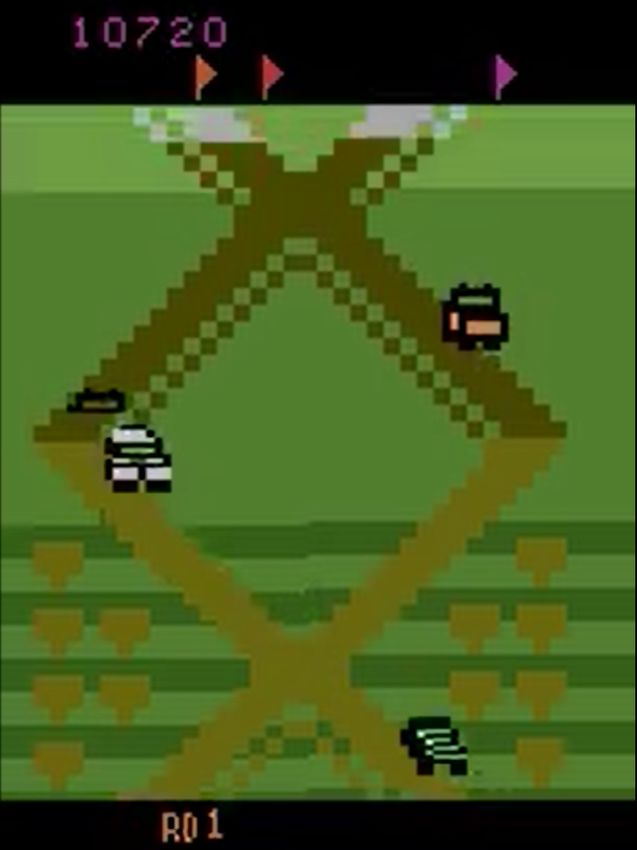
Under review as a conference paper at ICLR 2021

Considering the wide spectrum of deep reinforcement learning algorithm deployment it is crucial
to investigate the resilience of these algorithms before they are used in real world application
domains. Moreover, adversarial formulations are a first step to understand these algorithms and build
generalizable, reliable and robust deep reinforcement learning agents. Therefore, in this paper we
study adversarial attack formulations for deep reinforcement learning agents and make the following
contributions:

       • We define the optimal myopic adversary, whose aim is to minimize the value of the action
         taken by the agent in each state, and formulate the optimization problem that this adversary
         seeks to solve.
       • We introduce a differentiable approximation for the optimal myopic adversarial formulation.
       • We compare the impact results of our attack formulation to previous formulations in different
         games in the Atari environment.
       • We show that the new formulation finds a better direction for the adversarial perturbation
         and increases the attack impact for bounded perturbations. (Conversely, our formulation
         decreases the magnitude of the pertubation required to efficiently achieve a significant
         impact.)

2     R ELATED W ORK AND BACKGROUND

2.1   A DVERSARIAL R EINFORCEMENT L EARNING

Adversarial reinforcement learning is an active line of research directed towards discovering the
weaknesses of deep reinforcement learning algorithms. Gleave et al. (2020) model the interaction
between the agent and the adversary as a two player Markov game and solve the reinforcement
learning problem for the adversary via Proximal Policy Optimization introduced by Schulman et al.
(2017). They fix the victim agent’s policy and only allow the adversary to take natural actions to
disrupt the agent instead of using `p -norm bound pixel perturbations. Pinto et al. (2017) model the
adversary and the victim as a two player zero-sum discounted Markov game and train the victim in
the presence of the adversary to make the victim more robust. Mandlekar et al. (2017) use a gradient
based perturbation to make the agent more robust as compared to random perturbations. Huang et al.
(2017) and Kos & Song (2017) use the fast gradient sign method (FGSM) to show deep reinforcement
learning agents are vulnarable to adversarial perturbations. Pattanaik et al. (2018) use a gradient
based formulation to increase the robustness of deep reinforcement learning agents.

2.2   A DVERSARIAL ATTACK M ETHODS

Goodfellow et al. (2015) introduced the fast gradient method (FGM)

                                                     ∇x J(x, y)
                                    x∗ = x +  ·                   ,                                (1)
                                                   ||∇x J(x, y)||p

for crafting adversarial examples for image classification by taking the gradient of the cost function
J(x, y) used to train the neural network in the direction of the input. Here x is the input and y is the
output label for image classification. As mentioned in the previous section FGM was first adapted to
the deep reinforcement learning setting by Huang et al. (2017). Subsequently, Pattanaik et al. (2018)
introduced a variant of FGM, in which a few random samples are taken in the gradient direction,
and the best is chosen. However, the main difference between the approach of Huang et al. (2017)
and Pattanaik et al. (2018) is in the choice of the cost function J used to determine the gradient
direction. In the next section we will outline the different cost functions used in these two different
formulations.

2.3   A DVERSARIAL ATTACK F ORMULATIONS

In a bounded attack formulation for deep reinforcement learning, the aim is to try to find a perturbed
state sadv in a ball

                                                   2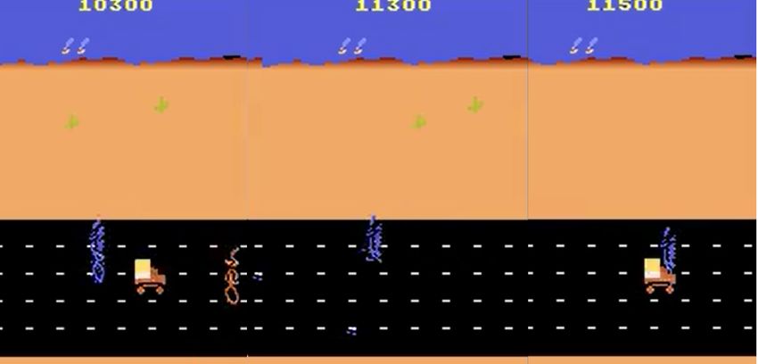
Under review as a conference paper at ICLR 2021

                                 D,p (s) = {sadv              ksadv − skp ≤ },                         (2)

that minimizes the expected cumulative reward of the agent. It is important to note that the agent
will always try to take the best action depending only on its perception of the state, and independent
from the unperturbed state. Therefore, in the perturbed state the agent will still choose the action,
a∗ (sadv ) = arg maxa Q(sadv , a), which maximizes the state action value function in state sadv .
It has been an active line of research to find the right direction for the adversarial perturbation in the
deep reinforcement learning domain. The first attack of this form was formulated by Huang et al.
(2017) and concurrently by Kos & Song (2017) by trying to minimize the probability of the best
possible action in the given state,

                                        a∗ (s) = arg max Q(s, a)
                                                           a
                                                                                                         (3)
                                            min           π(sadv , a∗ (s)).
                                        sadv ∈D,p (s)

Note that π(s, a) is the softmax policy of the agent given by

                                                                Q(s,a(s))
                                                     e             T
                                         πT (s, a) = P               Q(s,ak )
                                                                                ,                        (4)
                                                                 e      T
                                                           ak

where T is called the temperature constant. When the temperature constant is not relevant to the
discussion we will drop the subscript and use the notation π(s, a). It is important to note that π(s, a)
is not the actual policy used by the agent. Indeed the DRL agent deterministically chooses the action
a∗ maximizing Q(s, a) (or equivalently π(s, a)). The softmax operation is only introduced in order
to calculate the adversarial perturbation direction. Lin et al. (2017) formulated another attack with
unbounded perturbation based on the Carlini & Wagner (2017) attack where the goal is to minimize
the perturbation subject to choosing any action other than the best.

                                         min          ksadv − skp
                                     sadv ∈D,p (s)

                                     subject to       a∗ (s) 6= a∗ (sadv ).

Pattanaik et al. (2018) formulated yet another attack which aims to maximize the probability of the
worst possible action in the given state,

                                       aw (s) = arg min Q(s, a)
                                                           a
                                                                                                         (5)
                                            max          π(sadv , aw (s)),
                                        sadv ∈D,p (s)

and further showed that their attack formulation (5) is more effective than (3).
Pattanaik et al. (2018) also introduce the notion of targeted attacks to the reinforcement learning
domain. In their paper they take the cross entropy loss between the optimal policy in the given state
and their adversarial probability distribution and try to increase the probability of aw . However, just
trying to increase the probability of aw in the softmax policy i.e. π(sadv , aw ) is not sufficient to target
aw in the actual policy followed by the agent. In fact the agent can end up in a state where,

                                        π(sadv , aw ) > π(s, aw )
                                        aw 6= arg max π(sadv , a).                                       (6)
                                                      a

Although π(sadv , aw ) has increased, the action aw will not be taken. However, it might be still
possible to find a perturbed state s0adv for which,

                                                           3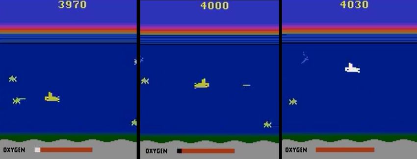
Under review as a conference paper at ICLR 2021

                                               π(sadv , aw ) > π(s0adv , aw )
                                               aw = arg max π(s0adv , a).                                                  (7)
                                                            a

Therefore, maximizing the probability of taking the worst possible action in the given state is not
actually the right formulation to find the correct direction for adversarial perturbation.

3     O PTIMAL M YOPIC A DVERSARIAL F ORMULATION
To address the problem described in Section 2.3 we define an optimal myopic adversary to be an
adversary which aims to minimize the value of the action taken by the agent myopically for each
state. The value of the action chosen by the agent in the unperturbed state is Q(s, a∗ (s)), and the
value (measured in the unperturbed state) of the action chosen by the agent under the influence of the
adversarial observation is Q(s, a∗ (sadv )). The difference between these is the actual impact of the
attack. Therefore, in each state s the optimal myopic adversary must solve the following optimization
problem

                                      arg max [Q(s, a∗ (s)) − Q(s, a∗ (sadv ))].                                           (8)
                                     sadv ∈D,p (s)

By (4), we may rewrite (8) in terms of the softmax policies π(s, a),

                                       arg max [π(s, a∗ (s)) − π(s, a∗ (sadv ))].                                          (9)
                                      sadv ∈D,p (s)

Since π(s, a∗ (s)) does not depend on sadv , (9) is equivalent to solving

                                              min       π(s, arg max{π(sadv , a)}).                                       (10)
                                       sadv ∈D,p (s)               a

3.1     E FFICIENT A PPROXIMATION OF O PTIMAL M YOPIC A DVERSARIAL F ORMULATION

Having an arg max operator in the cost function is unpleasant, since it is non-differentiable. Instead
we can approximate arg max by decreasing the temperature T for πT (sadv , a),

                                     lim πTadv (sadv , a) = 1arg max{π(sadv ,a0 )} (a).                                   (11)
                                    Tadv →0                             a0

                                                                                                                ∗
The intuition for (11) is that, by (3), as we decrease the temperature the value of e(Q(s,a )/Tadv ) for the
action a∗ which maximizes Q(s, a) will dominate the other actions. Thus π(s, arg maxa {π(sadv , a)})
can be approximated by,

                                                                    π(s, a) · 1arg max{π(sadv ,a0 )} (a)
                                                             X
                        π(s, arg max{π(sadv , a)}) =                                                                      (12)
                                a                                                     a0
                                                                a
                                                                        X
                                                          = lim               π(s, a) · πTadv (sadv , a)                  (13)
                                                             Tadv →0
                                                                          a

Therefore, our original optimization problem can be expressed as,

                                                                                      X
        min          π(s, arg max{π(sadv , a)}) =                   min         lim            π(s, a) · πTadv (sadv , a). (14)
    sadv ∈D,p (s)          a                                sadv ∈D,p (s) Tadv →0
                                                                                           a

In practice we will not be decreasing Tadv to 0 as this would be equal to applying the non-differentiable
argmax operation. Instead we will replace the arg max operation with the approximation πTadv (s, a)

                                                                4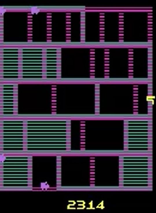
Under review as a conference paper at ICLR 2021

Figure 1: Games used in the experiments from Atari Arcade Environment. Games from left to right
in order: Roadrunner, Riverraid, Bankkeist, Seaquest, Amidar, Beamrider, Pong and UpandDown.

for a small value of Tadv . In general it is not guarenteed that the minimum of the cost function in
(14) with this approximation will be close to the minimum of the original cost function with the
arg max operation. To see why, note that this approximation is equivalent to first switching the limit
and minimum in (14) to obtain,
                                                      X
                              lim        min               π(s, a) · πTadv (sadv , a),             (15)
                             Tadv →0 sadv ∈D,p (s)
                                                       a

and second replacing the limit with a small value of Tadv . There are two possible issues with this
approach. First of all, due to the non-convexity of the minimand, exchanging the limit and minimum
may not yield an equality between (14) and (15). Secondly, even if this exchange is legitimate, it is
not clear how to choose a sufficiently small value for Tadv in order to obtain a good approximation to
(15). However, we show in our experiments that using this approximation in the cost function gives
state-of-the-art results.
There is another caveat which applies to all myopic adversaries including those in prior work. The
Q-value is a good estimate of the discounted future rewards of the agent, only assuming that the agent
continues to take the action maximizing the Q-value in future states. Since myopic attacks are applied
in each state, this may make minimizing the Q-value a non-optimal attack strategy when the future is
taken into account. There is also always the risk that the agent’s Q-value is miscalibrated. However,
our experiments show that our myopic formulation performs well despite these potential limitations.

3.2   E XPERIMENTAL S ETUP

In our experiments we averaged over 10 episodes for each Atari game (Bellemare et al., 2013) in
Figure 1 from the Open AI gym environment (Brockman et al., 2016). Agents are trained with
Double DQN (Wang et al., 2016). We compared the attack impact of our Myopic formulation with
the previous formulations of Huang et al. (2017) and Pattanaik et al. (2018). The attack impact has
been normalized by comparing an unattacked agent, which chooses the action corresponding to the
maximum state-action value in each state, with an agent that chooses the action corresponding to
the minimum state-action value in each state. Formally, let Rmax be the average return for the agent
who always chooses the best action in a given state, let Rmin be the average return for the agent who
always chooses the worst possible action in a given state, and let Ra be the average return of the agent
under attack. We define the impact I, as

                                                       Rmax − Ra
                                             I=                   .                                (16)
                                                      Rmax − Rmin
This normalization was chosen because we observed that in Atari environments agents can still collect
stochastic rewards even when choosing the worst possible action in each state until the game ends.
See more details of the setup in Appendix A.2.

3.3   A DVERSARIAL T EMPERATURE

Based on the discussion in Section 3 we expect that as Tadv decreases the function in (14) becomes
a better approximation of the arg max function. Thus this results in a higher attack impact as Tadv
decreases. However, after a certain threshold the function in (14) becomes too close to the arg max

                                                           5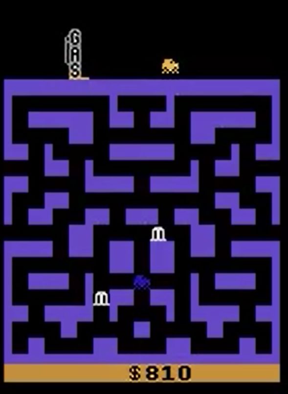
Under review as a conference paper at ICLR 2021

Figure 2: Attack impacts vs temperature constant for different games `2 -norm bound with  = 10−8 .
Left: Riverraid. Middle: Roadrunner. Right: Seaquest.

Table 1: Left: Attack impacts for three attack formulations with `2 norm bound and  = 10−8 . Right:
Attack impacts for three attack formulations with `1 norm bound and  = 10−8 .

 Games          Huang        Pattanaik    Myopic          Games          Huang        Pattanaik     Myopic
 Amidar        0.048±0.19   0.514±0.29   0.932±0.02       Amidar        0.039±0.22   0.502±0.32    0.941±0.03
 Bankheist     0.111±0.14   0.373±0.15   0.624±0.08       Bankheist    -0.014±0.07   0.0411±0.12   0.596±0.06
 Beamrider      0.083±0.3   0.455±0.27   0.663±0.13       Beamrider    -0.052±0.55   0.374±0.13    0.581±0.15
 Riverraid    -0.079±0.19   0.379±0.27   0.589±0.12       Riverraid    0.062±0.29     0.369±0.21    0.549±0.1
 RoadRunner    0.187±0.16   0.387±0.16   0.557±0.11       RoadRunner   0.153±0.12     0.453±0.15   0.482±0.07
 Pong          0.0±0.016    0.067±0.06   0.920±0.08       Seaquest     0.386±0.25     0.468±0.23   0.576±0.17
 Seaquest      0.305±0.26   0.524±0.23   0.697±0.16       Pong         0.000±0.02     0.043±0.03   0.916±0.09
 UpNDown        0.074±0.3   0.476±0.16   0.865±0.06       UpNDown      -0.007±0.28    0.436±0.28   0.892±0.07

Figure 3: Attack impact vs logarithm base 10 of `2 -norm bound. Left: Amidar. Middle: Pong. Right:
UpNDown.

function which is non-differentiable. Therefore, in practice, beyond this threshold the quality of the
solutions given by the gradient based optimization will decrease, and so the attack impact will be
lower. Indeed this can be observed in Figure 2. In our experiments we chose Tadv to maximize the
impact by grid search.

3.4   I MPACT C OMPARISON FOR `p - NORM B OUNDED P ERTURBATIONS

Table 1 shows the mean and standard deviation of the impact values under `1 and `2 -norm bounds.
The tables show that the proposed attack results in higher mean impact for all games and under all
norms, and it results in a lower standard deviation almost always. In particular, this is an indication
that our myopic attack formulation achieves higher impact more consistently than the previous
formulations. More results on `∞ -norm bound can be found in Section A.1 of the Appendix.
Figure 3 shows the attack impact as a function of the perturbation bound for each formulation in
three games. As  decreases, our myopic formulation exhibits higher impact relative to the other
formulations. Recall that Goodfellow et al. (2015) argue that small adversarial perturbations shift
the input across approximately linear decision boundaries learned by neural networks. Therefore,
having a higher impact with smaller norm bound is evidence that our myopic formulation finds a
better direction (i.e. one that points more directly at such a decision boundary) to search for the
perturbation.

                                                      6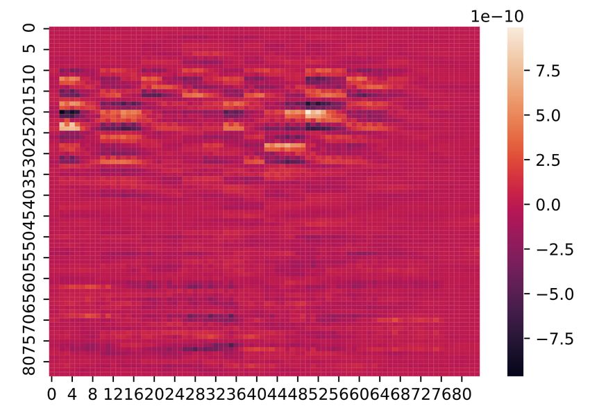
Under review as a conference paper at ICLR 2021

               (a) Pong                             (b) BankHeist                         (c) UpNDown

            (d) RiverRaid                          (e) Amidar                          (f) BeamRider

Figure 4: Up: Average empirical probabilities of ranked actions for three different formulations. Left:
Bankheist. Middle: Pong. Right: UpNDown. Down: Expected probability of ranked actions of three
different formulations. Left: Riverraid. Middle: Amidar. Right: BeamRider.

3.5   D ISTRIBUTION ON ACTIONS TAKEN

In order to understand the superior performance of the proposed adversarial formulation it is worth-
while to analyze the distribution of the actions taken by the agents under attack. For each formulation,
we recorded the empirical probability p(s, ak ) that the attacked agent chooses the k th ranked action
ak . The ranking of the actions is according to their value in the unperturbed state. Without perturba-
tion agents would always take their first ranked action, any deviation from this is a consequence of the
adversarial perturbations. We average these values over 10 episodes to obtain the average empirical
probability that the k th action is taken Ee∼ρ [p(s, ak )]. Here ρ is the distribution on the episodes e of
the game induced by the stochastic nature of the Atari games. We plot the results in Figure 4.
The legends in Figure 4 show the average empirical probabilities of taking the best action a∗ . It
can be seen that in general Ee∼ρ [p(s, a∗ )] is lower and Ee∼ρ [p(s, aw )] is higher for our Myopic
formulation when compared to other attack formulations. We realized that the formulations which
have higher impact at the end of the game might still be choosing the best action more often than the
ones which have lower attack impact as shown in the legend of Figure 4 for the Pong game. In this
case both Huang et al. (2017) and Pattanaik et al. (2018) cause the agent to choose the best action a∗
less frequently than our formulation, but still end up with lower impact. If we look at Figure 4 it can
                          nd
be seen that Ee∼ρ [p(s, a2 )] is much higher for both Huang et al. (2017) and Pattanaik et al. (2018)
compared to our Myopic formulation. However, the key to achieving a greater impact is to cause the
agent to choose the lowest ranked actions more frequently. As can be seen from Figure 4, our Myopic
formulation does this more successfully. More detailed results can be found in Appendix A.5.

3.6   S TATE -ACTION VALUES OVER T IME

In this section we investigate state-action values of the agents over time without an attack, under
attack with the Pattanaik et al. (2018) formulation, and under attack with our myopic formulation.
In Table 2 it is interesting to observe that under attack the mean of the state-action values over the
episodes might be higher despite the average return being lower. One might think that an attack
with greater impact might visit lower valued states on average. However, in our experiments we
have found that the gap between Ee∼ρ [Q(s, a∗ (s))] and Ee∼ρ [Q(s, a∗ (sadv )] relative to the gap

                                                    7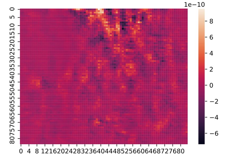
Under review as a conference paper at ICLR 2021

Table 2: Average Q-values for the best, worst, the adversarial actions and impacts, loss in the Q-values
caused by the adversarial influence, and impacts over the episodes.

                                E[Q(s, a∗ (s))]   E[Q(s, a∗ (sADV )]   E[Q(s, aw )]   QLOSS    I MPACT
         R IVERRAID
         U NATTACKED                 9.724                -              8.911           0        0
         H UANG ET. AL               9.656              9.653            8.8577       0.0039   -0.079
         PATTANAIK ET.   AL .       10.092             10.072            9.341        0.0258    0.379
         M YOPIC                    10.013             9.977             9.283        0.0495    0.589
         S EAQUEST
         U NATTACKED                 9.724                -              8.911           0       0
         H UANG ET. AL             10.6787            10.6787            10.100       0.0043   0.305
         PATTANAIK ET.   AL .       10.092             10.072            9.341        0.0267   0.524
         M YOPIC                    10.013             9.977             9.283        0.0506   0.697
         BANKHEIST
         U NATTACKED                6.6863                -              5.9273          0       0
         H UANG ET. AL               6.602             6.5998             5.907       0.0039   0.111
         PATTANAIK ET.   AL .       6.0517             6.0403             5.604       0.025    0.373
         M YOPIC                    5.9351             5.9153            5.5520       0.517    0.624
         A MIDAR
         U NATTACKED                0.1188                -             -0.1487          0       0
         H UANG ET. AL               0.115              0.114            -0.147       0.0049   0.048
         PATTANAIK ET.   AL .        0.139              0.138            -0.163       0.0466   0.514
         M YOPIC                    0.2239             0.1953           -0.2564       0.059    0.932

between Ee∼ρ [Q(s, a∗ (s))] and Ee∼ρ [Q(s, aw )] is a much more significant factor in determining the
magnitude of the impact. Therefore, we define the quantity

                                    Ee∼ρ [Q(s, a∗ (s))] − Ee∼ρ [Q(s, a∗ (sadv )]
                          Qloss =                                                .                       (17)
                                      Ee∼ρ [Q(s, a∗ (s))] − Ee∼ρ [Q(s, aw )]

Observe in Table 2 the magnitudes of Ee∼ρ [Q(s, a∗ (s))], Ee∼ρ [Q(s, aw )], and Ee∼ρ [Q(s, a∗ (sadv )]
are not strictly correlated to the impacts for each formulation. However, Qloss is always higher for
our Myopic attack compared to the previous formulations. Recall that in Equation (3), our original
optimization problem was designed to maximize the gap between Q(s, a∗ (s)) and Q(s, a∗ (sadv )) in
each state. The results in Table 2 are evidence both that we achieve this original goal and that solving
our initial optimization problem for each state leads to lower average return at the end of the game.
More results on this matter can be found in Appendix A.4.
The mean Q-value per episode under attack increases in some games. We believe that this may be
due to the fact that the Q-value in a given state is only an accurate representation of the expected
rewards of an unattacked agent. When the agent is under attack, there might be states with high
Q-value which are dangerous for the attacked agent (e.g. states where the attack causes the agent to
immediately lose the game). More results can be found in Appendix A.3.

4    F UTURE E XTENSIONS TO C ONTINUOUS ACTION S ETS

We note in this section that, at least from a mathematical point of view, it is possible to extend our
formulation to continuous control tasks. Observe that the adversarial objective in (8) applies to
continuous control problems too. The difficulty we are describing in (10) is not an issue in continuous
control tasks. For instance, in Deep Deterministic Policy Gradient (DDPG) or Proximal Policy
Optimization (PPO) the adversarial policy is already approximated by the actor network µθ (s). That
is: a∗ (sadv ) = µθ (sadv ). Unlike in the case of discrete action sets, this means that the solution to the
problem in (8) can be approximated through gradient descent following,

                                                  ∂Q(s, a)
                       ∇(Q(s, µθ (sadv )) =                |a=µθ (sadv ) · ∇(µθ (sadv )),                (18)
                                                    ∂a

                                                        8
Under review as a conference paper at ICLR 2021

where the gradient is taken with respect to sadv . In a way it is actually easier to construct the
adversarial examples in continuous control tasks because the learning algorithm already produces a
differentiable approximation µθ (s) to the argmax operation used in action selection. In our paper we
focused on the derivation for the case of a discrete action set because the optimization problem in
(10) is harder to solve.

5   C ONCLUSION
In this paper we studied formulations of adversarial attacks on deep reinforcement learning agents
and defined the optimal myopic adversary which incorporates the action taken in the adversarial state
into the cost function. By introducing a differentiable approximation to the value of the action taken
by the agent under the influence of the adversary we find a direction for adversarial perturbation
which more effectively decreases the Q-value of the agent in the given state. In our experiments we
demonstrated the efficacy of our formulation as compared to the previous formulations in the Atari
environment for various games. Adversarial formulations are inital steps towards building resilient
and reliable DeepRL agents, and we believe our adversarial formulation can help to set a new baseline
towards the robustification of DeepRL algorithms.

R EFERENCES
Marc G Bellemare, Yavar Naddaf, Joel Veness, and Michael. Bowling. The arcade learning environ-
 ment: An evaluation platform for general agents. Journal of Artificial Intelligence Research., pp.
 253–279, 2013.
Greg Brockman, Vicki Cheung, Ludwig Pettersson, Jonas Schneider, John Schulman, Jie Tang, and
  Wojciech Zaremba. Openai gym. arXiv:1606.01540, 2016.
Nicholas Carlini and David Wagner. Towards evaluating the robustness of neural networks. In 2017
  IEEE Symposium on Security and Privacy (SP), pp. 39–57, 2017.
Xianfu Chen, Honggang Zhang, Celimuge Wu, Shiwen Mao, Yusheng Ji, and Medhi. Bennis.
  Optimized computation offloading performance in virtual edge computing systems via deep
  reinforcement learning. IEEE Internet of Things Journal 6, pp. 4005–4018, 2018.
Sandeep Chinchali, Pan Hu, Tianshu Chu, Manu Sharma, Manu Bansal, Rakesh Misra, Marco
  Pavone, and Sachin. Katti. Cellular network traffic scheduling with deep reinforcement learning.
  In Thirty-Second AAAI Conference on Artificial Intelligence., 2018.
Tianshu Chu, Sandeep Chinchali, and Sachin Katti. Multi-agent reinforcement learning for networked
  system control. In Proceedings of the International Conference on Learning Representations
  (ICLR), 2020.
Liu Daochang and Tingting. Jiang. Deep reinforcement learning for surgical gesture segmentation
  and classification. In International conference on medical image computing and computer-assisted
  intervention., pp. 247–255.Springer, Cham, 2018.
Alexey Dosovitsky, German Ros, Felipe Codevilla, Antonio Lopez, and Vladlen Koltun. Carla: An
  open urban driving simulator. In Proceedings of the Conference on Robot Learning (CoRL), 78:
  1–16, 2017.
Jiajun Duan, Di Shi, Ruisheng Diao, Haifeng Li, Zhiwei Wang, Bei Zhang, Desong Bian, and Zhehan.
   Yi. Deep-reinforcement-learning-based autonomous voltage control for power grid operations.
   IEEE Transactions on Power Systems, 2019.
Florin-Cristian Ghesu, Bogdan Georgescu, Yefeng Zheng, Sasa Grbic, Andreas Maier, Joachim
  Hornegger, and Dorin. Comaniciu. Multi-scale deep reinforcement learning for real-time 3d-
  landmark detection in ct scans. IEEE transactions on pattern analysis and machine intelligence
  41, pp. 176–189, 2017.
Adam Gleave, Michael Dennis, Cody Wild, Kant Neel, Sergey Levine, and Stuart Russell. Adver-
  sarial policies: Attacking deep reinforcement learning. International Conference on Learning
 Representations ICLR, 2020.

                                                  9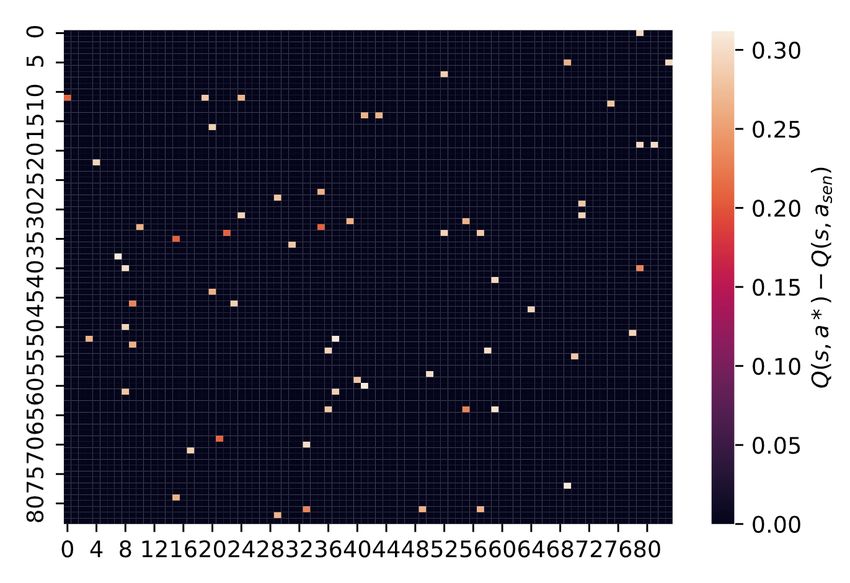
Under review as a conference paper at ICLR 2021

Ian Goodfellow, Jonathan Shelens, and Christian Szegedy. Explaning and harnessing adversarial
  examples. International Conference on Learning Representations, 2015.
Shixiang Gu, Timothy Holly, Ethan andLillicrap, and Sergey. Levine. Deep reinforcement learning for
  robotic manipulation with asynchronous off-policy updates. In 2017 IEEE international conference
  on robotics and automation (ICRA), pp. 3389–3396, 2017.
Awni Hannun, Carl Case, Jared Casper, Bryan Catanzaro, Diamos Greg, Erich Else, Ryan Prenger,
 Sanjeev Satheesh, Sengupta Shubho, Ada Coates, and Andrew Ng. Deep speech: Scaling up
 end-to-end speech recognition. arXiv preprint arXiv:1412.5567, 2014.
Charlie Hou, Mingxun Zhou, Yan Ji, Phil Daian, Florian Tramer, Giulia Fanti, and Ari. Juels. Squirrl:
  Automating attack discovery on blockchain incentive mechanisms with deep reinforcement learning.
  arXiv preprint arXiv:1912.01798, 2019.
Qiuhua Huang, Renke Huang, Weituo Hao, Tan Jie, Rui Fan, and Zhenyu. Huang. Adaptive power
  system emergency control using deep reinforcement learning. IEEE Transactions on Smart Grid
  (2019)., 2019.
Sandy Huang, Nicholas Papernot, Yan Goodfellow, Ian an Duan, and Pieter Abbeel. Adversarial
  attacks on neural network policies. Workshop Track of the 5th International Conference on
  Learning Representations, 2017.
Nathan Jay, Noga Rotman, Michael Godfrey, Brighten Schapira, and Aviv. Tamar. A deep reinforce-
  ment learning perspective on internet congestion control. In International Conference on Machine
  Learning, pp. 3050–3059, 2019.
Dmitry Kalashnikov, Alex Irpan, Peter Pastor, Julian Ibarz, Alexander Herzog, Eric Jang, Deirdre
 Quillen, Ethan Holly, Mrinal Kalakrishnan, Vincent Vanhoucke, and Sergey Levine. Qt-opt:
 Scalable deep reinforcement learning for vision-based robotic manipulation. arXiv preprint
 arXiv:1806.10293, 2018.
Jernej Kos and Dawn Song. Delving into adversarial attacks on deep policies. International
  Conference on Learning Representations, 2017.
Alex Krizhevsky, Ilya Sutskever, and Geoffrey E. Hinton. Imagenet classification with deep convolu-
  tional neural networks. Advances in neural information processing systems, 2012.
Timothy P Lillicrap, Jonathan J Hunt, Alexander Pritzel, Nicolas Heess, Tom Erez, Yuval Tassa, David
  Silver, and Daan. Wierstra. Continuous control with deep reinforcement learning. arXivpreprint
  arXiv:1509.02971, 2015.
Yen-Chen Lin, Hong Zhang-Wei, Yuan-Hong Liao, Meng-Li Shih, ing-Yu Liu, and Min Sun. Tactics
  of adversarial attack on deep reinforcement learning agents. Proceedings of the Twenty-Sixth
  International Joint Conference on Artificial Intelligence, pp. 3756–3762, 2017.
Ajay Mandlekar, Yuke Zhu, Animesh Garg, Li Fei-Fei, and Silvio Savarese. Adversarially robust
  policy learning: Active construction of physically-plausible perturbations. In Proceedings of the
  IEEE/RSJ International Conference on Intelligent Robots and Systems (IROS), pp. 3932–3939,
  2017.
Volodymyr Mnih, Koray Kavukcuoglu, David Silver, Andrei A Rusu, Joel Veness, arc G Bellemare,
  Alex Graves, Martin Riedmiller, Andreas Fidjeland, Georg Ostrovski, Stig Petersen, Charles
  Beattie, Amir Sadik, Antonoglou, Helen King, Dharshan Kumaran, Daan Wierstra, Shane Legg,
  and Demis Hassabis. Human-level control through deep reinforcement learning. Nature, 518:
  529–533, 2015.
Volodymyr Mnih, Adria Badia Puigdomenech, Mehdi Mirza, Alex Graves, Timothy Lillicrap, Tim
  Harley, David Silver, and Koray. Kavukcuoglu. Asynchronous methods for deep reinforcement
  learning. In International Conference on Machine Learning, pp. 1928–1937, 2016.
Laura Noonan. Jpmorgan develops robot to execute trades. Financial Times, pp. 1928–1937, July
  2017.

                                                10
Under review as a conference paper at ICLR 2021
Anay Pattanaik, Zhenyi Tang, Shuijing Liu, and Bommannan Gautham. Robust deep reinforce-
ment learning with adversarial attacks. In Proceedings of the 17th International Conference on
Autonomous Agents and MultiAgent Systems, pp. 2040–2042, 2018.
Lerrel Pinto, James Davidson, Rahul Sukthankar, and Abhinav Gupta. Robust adversarial reinforce-
ment learning. International Conference on Learning Representations ICLR, 2017.
Mariya Popova, Olexandr Isayev, and Alexander. Tropsha. Deep reinforcement learning for de novo
drug design. Science advances 4, 78, 2018.
John Schulman, Sergey Levine, Pieter Abbeel, Michael Jordan, and Philipp Moritz. Trust region
policy optimization. In Proceedings of the 32nd International Conference on Machine Learning
(ICML-15), 2015.
John Schulman, Filip Wolski, Prafulla Dhariwal, Alec Radford, and Oleg. Klimov. Proximal policy
optimization algorithms. arXiv:1707.06347v2 [cs.LG]., 2017.
Ilya Sutskever, Oriol Vinyals, and Quoc V. . Le. Sequence to sequence learning with neural networks.
Advances in neural information processing systems, 2014.
Christian Szegedy, Wojciech Zaremba, Ilya Sutskever, Joan Bruna, Dimutru Erhan, Ian Goodfellow,
and Rob Fergus. Intriguing properties of neural networks. In Proceedings of the International
Conference on Learning Representations (ICLR), 2014.
Brijen Thananjeyan, Animesh Garg, Sanjay Krishnan, Carolyn Chen, Lauren Miller, and Ken. Gold-
berg. Multilateral surgical pattern cutting in 2d orthotropic gauze with deep reinforcement learning
policies for tensioning. In 2017 IEEE International Conference on Robotics and Automation
(ICRA)., pp. 2371–2378, 2017.
Huan-Hsin Tseng, Sunan Cui Yi Luo, Chien Jen-Tzung, Randall K, Ten Haken, and Issam El Naqa.
Deep reinforcement learning for automated radiation adaptation in lung cancer. Medical Physics,
(12):6690–6705, 2017.
Ziyu Wang, Tom Schaul, Matteo Hessel, Hado Van Hasselt, Marc Lanctot, and Nando. De Freitas.
Dueling network architectures for deep reinforcement learning. Internation Conference on Machine
Learning ICML., pp. 1995–2003, 2016.
11Under review as a conference paper at ICLR 2021
A A PPENDIX
A.1 `∞ - NORM B OUND
Table 3: Attack impacts for three attack formulations with `∞ norm bound and = 10−8 .
G AMES H UANG PATTANAIK M YOPIC
A MIDAR 0.208±0.14 0.290±0.37 0.536±0.25
BANKHEIST 0.197±0.12 0.410±0.09 0.527±0.16
B EAMRIDER 0.258±0.27 0.279±0.26 0.327±0.19
R IVERRAID -0.081±0.26 0.323±0.27 0.429±0.29
ROAD RUNNER 0.125±0.16 0.445±0.13 0.553±0.11
P ONG -0.002±0.01 0.065±0.03 0.086±0.04
S EAQUEST 0.344±0.25 0.449±0.24 0.450±0.23
U P ND OWN 0.244±0.28 0.369±0.4 0.532±0.16
One observation from these results is that the myopic formulation performs worse in the `∞ -norm
bound than it does in the `1 -norm bound and the `2 -norm bound when = 10−8 . A priori one might
expect the performance of the myopic formulation to best in the `∞ -norm bound because the unit
`∞ ball contains the unit balls of the `1 and `2 norms. To investigate this further we examined the
behaviour of `2 -norm bound and `∞ -norm bound while varying in Figure (5). Observe that at very
small scales the `2 -norm bounded perturbation has larger impact, but at larger scales the `∞ -norm
bounded perturbation generally performs better than the `2 -norm bounded perturbation. We link this
phenomenon to the decision boundary behaviour in different scales.
Figure 5: Left: Impact change with varying for `∞ -norm bounded and `2 -norm bounded perturbation
in Myopic formulation for Roadrunner game. Right: Impact change with varying for `∞ -norm
bounded and `2 -norm bounded perturbation in Myopic formulation for Bankheist game.
Recall that in the `2 -norm bound we use a perturbation in the gradient direction of length . However,
in the `∞ -norm bound we use a perturbation given by times the sign of the gradient. This
corresponds to the `∞ -norm bounded perturbation which causes the maximum possible change for a
linear function. Compared to previous formulations decreasing the temperature in the softmax makes
our objective function more nonlinear. Thus, at smaller scales it is crucial for the perturbation to be
in the exact direction of the gradient, since the decision boundary behaves nonlinearly. However, at
larger scales the decision boundary is approximately linear, which gives a better result in the `∞ -norm
bound.
12Under review as a conference paper at ICLR 2021
A.2 R ANDOMIZED I TERATIVE S EARCH AND I MPACTS
It can be seen from Figure 6 that the impact of the Pattanaik et al. (2018) formulation increases as n
increases, while our myopic formulation has a greater impact even when n is equal to 1. In particular,
this is again an indication that our cost function provides a better direction in which to search for
adversarial perturbations as compared to previous formulations.
Figure 6: Attack impacts vs number of iteration of random search (n) for Pong.
Our attack, as well as those of Huang et al. (2017) and Pattanaik et al. (2018), are all based on
computing the gradient of the respective cost functions and choosing a point along the gradient
direction to be the adversarial perturbation. Pattanaik et al. (2018) used a randomized search, where
n random points are sampled in the gradient direction and the one with lowest Q-value is chosen as
the perturbation. We follow Pattanaik et al. (2018) in using randomized search, and in all previous
results mentioned above we have set n = 5. In Table 4 we set n = 1 and compare the impact of the
three different formulations. Even in this more restrictive setting the performance of our formulation
remains high, while the performance of Pattanaik et al. (2018) degrades significantly. In particular,
this demonstrates that the gradient of our cost function is a better direction to find an adversarial
perturbation.
Table 4: Attack impacts for three different attack formulations with `2 norm bound and =
10−10 , n = 1
G AMES H UANG PATTANAIK M YOPIC
A MIDAR 0.050±0.25 0.138±0.31 0.941±0.02
BANKHEIST 0.189±0.13 0.247±0.15 0.487±0.09
B EAMRIDER 0.001±0.40 0.096±0.36 0.634±0.15
R IVERRAID 0.173±0.23 0.234±0.21 0.367±0.16
ROAD RUNNER 0.035±0.15 0.090±0.12 0.151±0.12
P ONG 0.173±0.23 0.014±0.03 0.887±0.09
S EAQUEST 0.321±0.14 0.290±0.4 0.502±0.22
U P ND OWN 0.475±0.24 0.615±0.10 0.911±0.04
A.3 G AMES AND AGENT B EHAVIOUR
In this section we share our observations on the behaviour of the trained agent under attack. In Figure
9 the agent performs well until it suddenly decides to stand still and wait for the enemy to arrive.
Similarly, in Figure 7 the trained agent performs quite well again until it decides to jump in front
of the truck. Finally, in Figure 8 the trained agent forgets to recharge its oxygen even though it is
earning many points from shooting the fishes and saving the divers.
13Under review as a conference paper at ICLR 2021
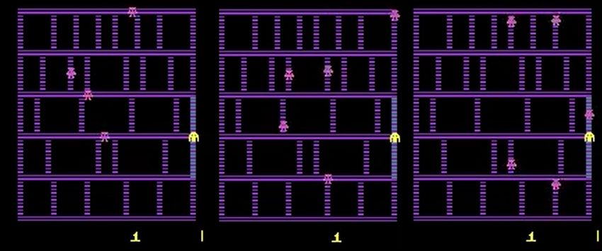
Figure 7: Example game from Atari Arcade Environment. The trained agent jumps in front of the car
even though the agent is not in the same lane with the car in RoadRunner game.
Figure 8: Example game from Atari Arcade Environment. The trained agent forgets to recharge its
oxygen even though its condition to recharge is not critical in Seaquest game.
Figure 9: Example game from Atari Arcade Environment. The trained agent just waits without
moving until the enemy reaches the agent in Amidar game.
14Under review as a conference paper at ICLR 2021
A.4 Q- VALUES OVER T IME
In this section we plot state-action values of the agents over time without an attack, under attack with
the Pattanaik et al. (2018) formulation, and under attack with our myopic formulation. In Figure 12 it
is interesting to observe that under attack the mean of the state-action values over the episodes might
be higher despite the average return being lower. .
Figure 10: State-action values vs time graph for Atari Arcade Game Seaquest. Left: Unattacked
agent. Middle: Pattanaik et al. (2018) adversarial formulation. Right: Myopic attack.
Figure 11: State-action values vs time graph for Atari Arcade Game Riverraid. Left: Unattacked
agent. Middle: Pattanaik et al. (2018) adversarial formulation. Right: Myopic attack.
Figure 12: State-action values vs time graph for Atari Arcade Game Bankheist. Left: Unattacked
agent. Middle: Pattanaik et al. (2018) adversarial formulation. Right: Myopic attack.
15Under review as a conference paper at ICLR 2021
A.5 R ESULTS ON AVERAGE EMPIRICAL PROBABILITIES OF ACTIONS
In this section we provide a detailed table on the average empirical probabilities of the best action a∗
and the worst action aw . It can be seen that in general Ee∼ρ [p(s, a∗ )] is lower and Ee∼ρ [p(s, aw )] is
higher for our Myopic formulation when compared to other attack formulations.
Table 5: Average empirical probabilities of a∗ and aw , and impacts for three different formulation for
Riverraid and BeamRider from Atari environment with `2 -norm bounded perturbation and = 10−8 .
Ee∼ρ [p(s, a∗ )] Ee∼ρ [p(s, aw )] Impact
Riverraid
Huang et. al. 0.9904±0.16 0.00226±0.0003 -0.0796 ±0.19
Pattanaik et. al. 0.9443±0.29 0.00285 ±0.0014 0.3797±0.27
Myopic 0.897±0.16 0.00369±0.0012 0.5897±0.12
BeamRider
Huang et. al. 0.989±0.244 0.0042±0.0005 0.0847±0.29
Pattanaik et. al. 0.948±0.320 0.0059±0.0023 0.4553±0.267
Myopic 0.826±0.195 0.0186±0.0048 0.6636±0.135
Amidar
Huang et. al. 0.9872±0.168 0.0011±0.0008 0.04762±0.111
Pattanaik et. al. 0.9377±0.348 0.0052±0.0022 0.5145±0.126
Myopic 0.8566±0.211 0.01225±0.0035 0.9320±0.198
BankHeist
Huang et. al. 0.9861±0.103 0.000357±0.00059 0.111±0.14
Pattanaik et. al. 0.9426±0.012 0.00261±0.0122 0.373±0.15
Myopic 0.8974±0.122 0.00433±0.0036 0.624±0.08
Pong
Huang et. al. 0.4684±0.056 0.0020±0.001 0.0±0.016
Pattanaik et. al. 0.5151±0.096 0.01028 ±0.004 0.067±0.06
Myopic 0.5695±0.159 0.06221±0.013 0.920±0.08
16Under review as a conference paper at ICLR 2021
A.6 S ENSITIVITY A NALYSIS
In this section we attempt to gain an insight into which pixels in the visited states are most sensitive
to perturbation. For each pixel i, j we measure the drop in the state action values when perturbing
that pixel by a small amount. Formally, let asen = arg maxa Q(ssensitivity , a), where ssensitivity is equal
to s except that a small perturbation γ has been added to the i, j-th pixel of s. Then we measure
Q(s, a∗ ) − Q(s, asen )) (19)
We plot the values from 19 in Figure 15. Note that any non-zero value (i.e. any lighter colored pixel
in the plot) indicates that a γ perturbation to the corresponding pixel will cause the agent to take an
action different from the optimal one. Lighter colored pixels correspond to larger drops in Q-value.
Figure 13: Sensitivity Analysis of RoadRunner. Left: γ = 10−8 . Right: γ = 10−10 .
17Under review as a conference paper at ICLR 2021
A.7 P ERTURBATION H EATMAPS
In thise section we demonstrate the heatmaps of the raw pixel perturbations and the preprocessed
frames from which the perturbations are computed.
Figure 14: Perturbation heatmaps of myopic formulation. Left: RoadRunner. Right: Riverraid.
Figure 15: Preprocessed frames. Left: RoadRunner. Right: Riverraid.
18You can also read