Learning and Planning for Temporally Extended Tasks in Unknown Environments
←
→
Page content transcription
If your browser does not render page correctly, please read the page content below
Learning and Planning for Temporally Extended Tasks in Unknown
                                                                            Environments
                                                                  Christopher Bradley1 , Adam Pacheck2 , Gregory J. Stein3 , Sebastian Castro1 ,
                                                                                   Hadas Kress-Gazit2 , and Nicholas Roy1

                                            Abstract— We propose a novel planning technique for sat-                        planning under uncertainty in this case as a Locally Observ-
                                         isfying tasks specified in temporal logic in partially revealed                    able Markov Decision Process (LOMDP) [7], a special class
                                         environments. We define high-level actions derived from the                        of Partially Observable Markov Decision Process (POMDP),
arXiv:2104.10636v2 [cs.RO] 28 Apr 2021

                                         environment and the given task itself, and estimate how each
                                         action contributes to progress towards completing the task. As                     which by definition includes our assumption of perfect range-
                                         the map is revealed, we estimate the cost and probability of                       limited perception. However, planning with such a model
                                         success of each action from images and an encoding of that                         requires a distribution over possible environment configura-
                                         action using a trained neural network. These estimates guide                       tions and high computational effort [8–10].
                                         search for the minimum-expected-cost plan within our model.                           Since finding optimal policies for large POMDPs is in-
                                         Our learned model is structured to generalize across environ-
                                         ments and task specifications without requiring retraining. We                     tractable in general [10], planning to satisfy temporal logic
                                         demonstrate an improvement in total cost in both simulated and                     specifications in full POMDPs has so far been limited to rel-
                                         real-world experiments compared to a heuristic-driven baseline.                    atively small environments or time horizons [11, 12]. Thus,
                                                                                                                            many approaches for solving tasks specified with temporal
                                                                                                                            logic often make simplifying assumptions about known and
                                                                    I. I NTRODUCTION                                        unknown space, or focus on maximizing the probability a
                                                                                                                            specification is never violated [13–17]. Accordingly, such
                                            Our goal is to enable an autonomous agent to find a                             strategies can result in sub-optimal plans, as they do not
                                         minimum cost plan for multi-stage planning tasks when the                          consider the cost of planning in unknown parts of the map.
                                         agent’s knowledge of the environment is incomplete, i.e.,                             A number of methods use learned policies to minimize the
                                         when there are parts of the world the robot has yet to observe.                    cost of completing tasks specified using temporal logic [18–
                                         Imagine, for example, a robot tasked with extinguishing a                          22]. However, due to the complexity of these tasks, many are
                                         small fire in a building. To do so, the agent could either find                    limited to fully observable small grid worlds [18–21] or short
                                         an alarm to trigger the building’s sprinkler system, or locate a                   time-horizons [22]. Moreover, for many of these approaches,
                                         fire extinguisher, navigate to the fire, and put it out. Temporal                  changing the specification or environment requires retraining
                                         logic is capable of specifying such complex tasks, and has                         the system. Recent work by Stein et al. [23] uses supervised
                                         been used for planning in fully known environments (e.g.,                          learning to predict the outcome of acting through unknown
                                         [2–6]). However, when the environment is initially unknown                         space, but is restricted to goal-directed navigation.
                                         to the agent, efficiently planning to minimize expected cost                          To address the challenges of planning over a distribution
                                         to solve these types of tasks can be difficult.                                    of possible futures, we introduce Partially Observable Tem-
                                            Planning in partially revealed environments poses chal-                         poral Logic Planner (PO-TLP). PO-TLP enables real-time
                                         lenges in reasoning about unobserved regions of space.                             planning for tasks specified in Syntactically Co-Safe Linear
                                         Consider our firefighting robot in a building it has never seen                    Temporal Logic (scLTL) [24] in unexplored, arbitrarily large
                                         before, equipped with perfect perception of what is in direct                      environments, using an abstraction based on a given task
                                         line of sight from its current position. Even with this perfect                    and partially observed map. Since completing a task may
                                         local sensing, the locations of any fires, extinguishers, and                      not be possible in known space, we define a set of dynamic
                                         alarms may not be known. Therefore, the agent must envision                        high-level actions based on transitions between states in our
                                         all possible configurations of unknown space—including the                         abstraction and available subgoals in the map—points on
                                         position of obstacles—to find a plan that satisfies the task                       the boundaries between free and unknown space. We then
                                         specification and, ideally, minimizes cost. We can model                           approximate the full LOMDP model such that actions either
                                                                                                                            successfully make their desired transitions or fail, splitting
                                            This work is supported by ONR PERISCOPE MURI N00014-17-1-                       future beliefs into two classes and simplifying planning. We
                                         2699 and the Toyota Research Institute (TRI). 1 CSAIL, Massachusetts
                                         Institute of Technology (MIT), Cambridge, MA 02142, USA ({cbrad,                   train a neural network from images to predict the cost and
                                         sebacf, nickroy}@mit.edu). 2 Sibley School of Mechanical and Aerospace             outcome of each action, which we use to guide a variant
                                         Engineering, Cornell University, Ithaca, NY 14850, USA ({akp84,                    of Monte-Carlo Tree Search (PO-UCT [25]) to find the best
                                         hadaskg}@cornell.edu). 3 Computer Science Department, George Mason
                                         University, Fairfax, VA 22030, USA (gjstein@gmu.edu). © 2021 IEEE.                 high-level action for a given task and observation.
                                         Personal use of this material is permitted. Permission from IEEE must                 Our model learns directly from visual input and can gener-
                                         be obtained for all other uses, in any current or future media, including          alize across novel environments and tasks without retraining.
                                         reprinting/republishing this material for advertising or promotional purposes,
                                         creating new collective works, for resale or redistribution to servers or lists,   Furthermore, since our agent continually replans as more
                                         or reuse of any copyrighted component of this work in other works.                 of the environment is revealed, we ensure both that the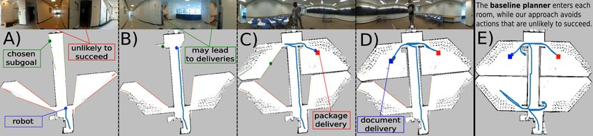
Fig. 1. Overview. (A) Given a task (e.g., (¬fire U extinguisher) ∧ ♦fire), we compute a DFA using [1] to represent the high-level steps needed
to accomplish the task. The robot operates in a partially explored environment with subgoals between observed (white) and unexplored (gray) space, and
regions labeled with propositions relevant to the task, e.g., extinguisher and fire. (B) We define high-level actions with a subgoal (e.g., s0 ), a DFA state z 0
(e.g., z0 ) which the robot must be in when arriving at the subgoal, and a state z 00 (e.g., z1 ) which the agent attempts to transition to in unknown space.
(C) For each possible action, we estimate its probability of success (PS ) and costs of success (RS ) and failure (RF ) using a neural network that accepts
a panoramic image centered on a subgoal, the distance to that subgoal, and an encoding of the transition from z 0 to z 00 (Sec. IV-A). (D) We estimate the
expected cost of each action with these estimates of PS , RS , and RF using PO-UCT search. (E) The agent selects an action with the lowest expected
cost, and moves along the path defined by that action, meanwhile receiving new observations, updating its map, and re-planning.

specification is never violated and that we find the optimal                      Deterministic Finite Automaton (DFA): A DFA, con-
trajectory if the environment is fully known. We apply PO-                        structed from an scLTL specification, is a tuple Dϕ =
TLP to multiple tasks in simulation and the real world,                           (Z, z0 , Σ, δD , F ). A DFA is composed of a set of states,
showing improvement over a heuristic-driven baseline.                             Z, with an initial state z0 ∈ Z. The transition function
                                                                                  δD : Z × 2Σ → Z takes in the current state, z ∈ Z,
                         II. P RELIMINARIES                                       and a letter ωi ∈ 2Σ , and returns the next state z ∈ Z in
Labeled Transition System (LTS): We use an LTS to                                 the DFA. The DFA has a set of accepting states, F ⊆ Z,
represent a discretized version of the robot’s environment.                       such that if the execution of the DFA on a finite word
An LTS T is a tuple (X, x0 , δT , w, Σ, l), where: X is a                         ω = ω0 ω1 . . . ωn ends in a state z ∈ F , the word belongs
discrete set of states of the robot and the world, x0 ∈ X                         to the language of the DFA. While in general LTL formulas
is the initial state, δT ⊆ X × X is the set of possible                           are evaluated over infinite words, the truth value of scLTL
transitions between states, the weight w : (xi , xj ) → R+                        can be determined over finite traces. Fig. 1A shows the DFA
is the cost incurred by making the transition (xi , xj ), Σ                       for (¬fire U extinguisher) ∧ ♦fire.
is a set of propositions with σ ∈ Σ, and the labeling
function l : X → 2Σ is used to assign which propositions                          Product Automaton (PA): A PA is a tuple
are true in state x ∈ X. An example LTS is shown in                               (P, p0 , δP , wP , FP ) which captures this combined behavior
Fig. 2A where Σ = {fire, extinguisher}, l(x3 ) =                                  of the DFA and LTS. The states P = X × Z keep track of
{extinguisher} and l(x4 ) = ∅. States x ∈ X refer to                              both the LTS and DFA states, where p0 = (x0 , z0 ) is the
physical locations, and labels like fire or extinguisher                          initial state. A transition between states is possible iff the
indicate whether there is a fire or extinguisher (or both) at                     transition is valid in both the LTS and DFA, and is defined
that location. A finite trajectory τ is a sequence of states                      by δP = {(pi , pj ) | (xi , xj ) ∈ δT , δD (zi , l(xj )) = zj }.
τ = x0 x1 . . . xn where (xi , xi+1 ) ∈ δT which generates a                      When the robot moves to a new state x ∈ X in the LTS, it
finite word ω = ω0 ω1 . . . ωn where each letter ωi = l(xi ).                     transitions to a state in the DFA based on the label l(x). The
                                                                                  weights on transitions in the PA are the weights in the LTS
Syntactically Co-Safe Linear Temporal Logic (scLTL):                              (wP (pi , pj ) = w(xi , xj )). Accepting states in the PA, FP ,
To specify tasks, we use scLTL, a fragment of Linear                              are those states with accepting DFA states (FP = X × F ).
Temporal Logic (LTL) [24]. Formulas are written over a
set of atomic propositions Σ with Boolean (negation (¬),                          Partially/Locally Observable Markov Decision Process:
conjunction (∧), disjunction (∨)) and temporal (next ( ),                         We model the world as a Locally Observable Markov Deci-
until (U), eventually (♦)) operators. The syntax is:                              sion Process (LOMDP) [7]—a Partially Observable Markov
     ϕ := σ | ¬σ | ϕ ∧ ϕ | ϕ ∨ ϕ |                ϕ | ϕ U ϕ | ♦ϕ,                 Decision Process (POMDP) [26] where space within line
                                                                                  of sight from our agent is fully observable—formulated as
where σ ∈ Σ, and ϕ is an scLTL formula. The semantics are                         a belief MDP, and written as the tuple (B, A, P, R). In a
defined over infinite words ω inf = ω0 ω1 ω2 . . . with letters                   belief MDP, B represents the belief over states in an MDP,
ωi ∈ 2Σ . Intuitively, ϕ is satisfied by a given ω inf at step                    which in our case are the states from the PA defined by
i if ϕ is satisfied at the next step (i + 1), ϕ1 Uϕ2 is satisfied                 a given task and environment. We can think of each belief
if ϕ1 is satisfied at every step until ϕ2 is satisfied, and ♦ϕ                    state as distributions over three entities bt = {bT , bx , bz }: the
is satisfied at step i if ϕ is satisfied at some step j ≥ i. For                  environment (abstracted as an LTS) bT , the agent’s position
the complete semantics of scLTL, refer to Kupferman and                           in that environment bx , and the agent’s progress through the
Vardi [24]. For example, (¬fire U extinguisher) ∧                                 DFA defined by the task bz . With our LOMDP formulation,
♦fire specifies the robot should avoid fire until reaching                        we collapse bx and bz to point estimates, and consider
the extinguisher and eventually go to the fire.                                   any states in T that have been seen by the robot as fully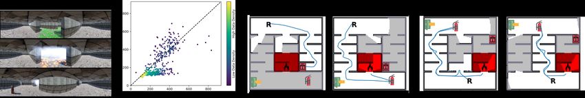
observable, allowing us to treat bT as a labeled occupancy
grid that is revealed as the robot explores. A is the set of
available actions from a given state in the PA, which at the
lowest level of abstraction are the feasible transitions given
by δP . P (bt+1 |bt , at ) and R(bt+1 , bt , at ) are the transition
probability and instantaneous cost, respectively, of taking an
action at to get from a belief bt to bt+1 .

   III. P LANNING IN UNKNOWN ENVIRONMENTS WITH
             CO - SAFE LTL SPECIFICATIONS
                                                                            Fig. 2. High-level actions. The robot (“R”) is in a partially explored
   Our objective is to minimize the total expected cost                     environment abstracted into an LTS with two subgoals s0 and s1 (A). As
of satisfying an scLTL specification in partially revealed                  the robot considers high-level actions at different stages of its plan (B), its
                                                                            color indicates belief of the DFA state (according to Fig. 1A). In this rollout,
environments. Using the POMDP model, we can represent                       the robot considers action as0 z0 z1 , and outcomes where it succeeds (C),
the expected cost of taking an action using a belief-space                  and fails (D). If successful, the robot has two actions available and considers
variant of the Bellman equation [26]:                                       as0 z1 z2 , which in turn could succeed (E) or fail (F).

                                                                            the set of DFA states that can be reached while traveling in
                     X                   h
       Q(bt , at ) =   P (bt+1 |bt , at ) R(bt+1 , bt , at )
                                                                            known space in the current belief bt to subgoal s ∈ St , and
                       bt+1
                                                               i     (1)    Znext (z 0 ) = {z 00 ∈ Z | ∃ωi ∈ 2Σ s.t. z 00 = δD (z 0 , ωi )} is the
                           +       min          Q(bt+1 , at+1 ) ,           set of DFA states that can be visited in one transition from z 0 .
                               at+1 ∈A(bt+1 )
                                                                            Fig. 2B illustrates an example of available high-level actions.
where Q(bt , at ) is the belief-action cost of taking action at                  When executing action asz0 z00 , the robot reaches subgoal
given belief bt . This equation can, in theory, be solved to find           s in DFA state z 0 , accumulating a cost D(bt , asz0 z00 )
the optimal action for any belief. However, given the size of               which is computed using Dijkstra’s algorithm in the
the environments we are interested in, directly updating the                known map. Once the robot enters the unknown space
belief in evaluation of Eq. (1) is intractable for two reasons.             beyond the subgoal, the action has some probability PS
First, due to the curse of dimensionality, the size of the belief           of successfully transitioning            from z 0 to z 00 , denoted as:
                                                                            PS (bt , asz0 z00 ) ≡ bt+1 P (bt+1 |asz0 z00 , bt )I[Z(bt+1 ) = z 00 ],
                                                                                                    P
grows exponentially with the number of states. Second, by
the curse of history, the number of iterations needed to solve              where Z(bt+1 ) refers to bz at the next time step
Eq. (1) grows exponentially with the planning horizon.                      and I[Z(bt+1 ) = z 00 ] is an indicator function for
                                                                            belief states where the agent has reached the DFA
A. Defining the Set of High-Level Actions                                   state z 00 . Each action has an expected cost of success
   To overcome the challenges associated with solving                       RS (b
                                                                             1
                                                                                  Pt , asz0 z00 ) such that RS (bt , asz0 z00 ) + D(bt , asz0 z00 ) ≡
Eq. (1), we first identify a set of discrete, high-level actions,                   bt+1 P (bt+1 |bt , asz z )R(bt+1 , bt , asz z )I[Z(bt+1 ) =
                                                                                                            0 00                 0 00
                                                                            PS
then build off an insight from Stein et al. [23]: that we can               z 00 ] and expected cost of failure RF (bt , asz0 z00 ), which is
simplify computing the outcome of each action by splitting                  equivalently defined for Z(bt+1 ) 6= z 00 and normalized with
                                                                                1
future beliefs into two classes—futures where a given action                1−PS . By estimating these values via learning (discussed in
is successful, and futures where it is not. Note that this                  Sec. IV), we can    P express the expected instantaneous cost of
abstraction over the belief space does not exist in general,                an action as           bt+1 P (bt+1 |bt , asz z )R(bt+1 , bt , asz z ) =
                                                                                                                         0 00                 0 00

and is enabled by our assumption of perfect local perception.               D + PS RS + (1 − PS )RF .
   To satisfy a task specification, our agent must take actions
to transition to an accepting state in the DFA. For exam-                   B. Estimating Future Cost using High-Level Actions
ple, given the specification (¬fire U extinguisher) ∧                           We now examine planning to satisfy a specification with
♦fire as in Fig. 1 and 2, the robot must first retrieve the                 minimum cost using these actions, remembering to consider
extinguisher and then reach the fire. If the task cannot be                 both the case where an action succeeds—the robot transitions
completed entirely in the known space, the robot must act                   to the desired state in the DFA—and when it fails. We refer
in areas that it has not yet explored. As such, our action set              to a complete simulated trial as a rollout. Since we cannot
is defined by subgoals S—each a point associated with a                     tractably update and maintain a distribution over maps during
contiguous boundary between free and unexplored space—                      a rollout, we instead keep track of the rollout history h =
and the DFA. Specifically, when executing an action, the                    [[a0 , o0 ], . . . , [an , on ]] (a sequence of high-level actions ai
robot first plans through the PA in known space to a subgoal,               considered during planning and their simulated respective
and then enters the unexplored space beyond that subgoal to                 outcomes oi = {success, failure}). Recall that, during
attempt to transition to a new state in the DFA.                            planning, we assume that the agent knows its position x in
   For belief state bt , action asz0 z00 defines the act of traveling       known space Tknown . Additionally, conditioned on whether
from the current state in the LTS x to reach subgoal s ∈                    an action asz0 z00 is simulated to succeed or fail, we assume
St at a DFA state z 0 , and then attempting to transition to                no uncertainty over the resulting DFA state, collapsing bz to
DFA state z 00 in unknown space. Our newly defined set of                   z 00 or z 0 , respectively. Therefore, for a given rollout history,
possible actions from belief state bt is: A(bt ) = {asz0 z00 | s ∈          the agent knows its position in known space and its state
St , z 0 ∈ Zreach (bt , s), z 00 ∈ Znext (z 0 )} where Zreach (bt , s) is   in the DFA. These assumptions, while not suited to solving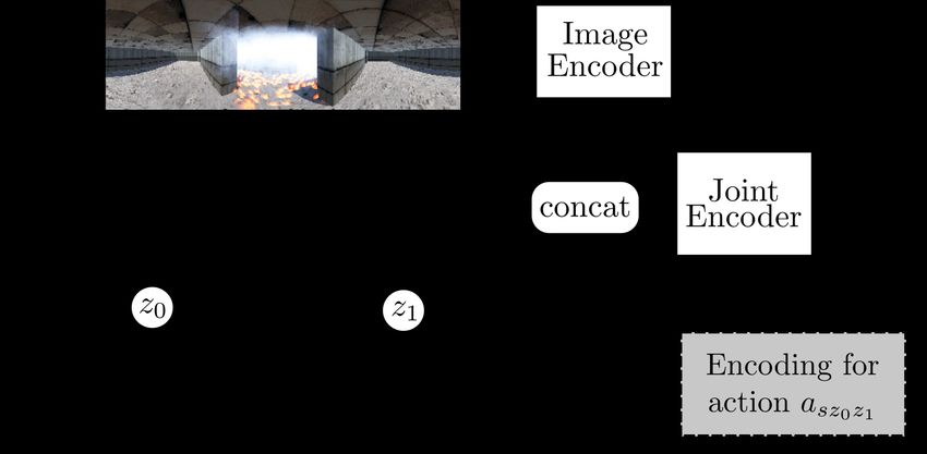
Algorithm 1 PO-TLP
Function PO-TLP(θ):                // θ: Network parameters
   b ← {bT0 , bx0 , bz0 }, Img ← Img0
   while True do
       if bz ∈ F then                    // In accepting state
            return SUCCESS
       a∗sz0 z00 ← H IGH L EVEL P LAN(b, Img, θ, A(b))
       b, Img ← ACTA ND O BSERVE (a∗sz0 z00 )
Function H IGH L EVEL P LAN (b, Img, θ, A(b)):
   for a ∈ A(b) do
        a.PS , a.RS , a.RF ← E ST P ROPS(b, a, Img | θ)
   a∗sz0 z00 ← PO-UCT(b, A(b))                                            Fig. 3. Neural network inputs and outputs. Estimating PS , RF , and
   return a∗sz0 z00                                                       RS for action asz0 z1 : attempting to reach an exit while avoiding fire.

POMDPs in general, fit within the LOMDP model.                            belief state bt+1 , allowing us to approximate it as follows:
                                                                              X
                                                                                  P (bt+1 |bt , asz0 z00 ) 0 min Q(bt+1 , a0 ) ≈
   During a rollout, the set of available future actions is                                                 a ∈A(bt+1 )
                                                                              bt+1
informed by actions and outcomes already considered in
h. For example, if we simulate an action in a rollout,                                PS (bh , asz0 z00 )      min        Q(bhS , aS )+         (2)
                                                                                                            aS ∈A(bhS )
and it fails, we should not consider that action a second
                                                                                      [1 − PS (bh , asz0 z00 )]      min        Q(bhF , aF ),
time. Conversely, we know a successful action would suc-                                                          aF ∈A(bhF )
ceed if simulated again in that rollout. In Fig. 2F, the
robot imagines its first action as0 z0 z1 succeeds, while its             where hS = h.append([asz0 z00 , success]) is the rollout
next action as0 z1 z2 fails, making the rollout history h =               history conditioned on a successful outcome (and hF is
[[as0 z0 z1 , success], [as0 z1 z2 , failure]]. When consider-            defined similarly for failed outcomes).
ing the next step of this rollout, the robot knows it can always             Our high-level actions and rollout history allow us to
find an extinguisher beyond s0 , and there is no fire beyond              approximate Eq. (1) with Eq. (3), a finite horizon problem.
s0 . To track this information during planning, we define a               Given estimates of PS , RS , and RF —which are learned as
rollout history-augmented belief bh = {Tknown , x, z, h},                 discussed in Sec. IV—we avoid explicitly summing over
which augments the belief with the actions and outcomes                   the distribution of all possible PAs, thereby reducing the
of the rollout up to that point. To reiterate, we maintain the            computational complexity of solving for the best action.
history-augmented belief bh only during planning, to avoid                  C. Planning with High-Level Actions using PO-UCT
the complexity of maintaining a distribution over possible
                                                                                  Eq. (3) demonstrates how expected cost can be computed
future maps from possible future observations during rollout.
                                                                            exactly using our high-level actions, given estimated values
                                                                            of PS , RS , and RF . However, considering every possible
   Using bh , we also define a rollout history-augmented ordering of actions as in Eq. (3) still involves significant
action set A(bh ), in which actions known to be impossible computational effort—exponential in both the number of
based on h are pruned, and with it, a rollout history- subgoals and the size of the DFA. Instead, we adapt Partially
augmented success probability PS (bh , asz0 z00 ) which is iden- Observable UCT (PO-UCT)[25], a generalization of Monte-
tically one for actions known to succeed. Furthermore, Carlo Tree-Search (MCTS) which tracks histories of actions
because high-level actions involve entering unknown space, and outcomes, to select the best action for a given belief
instead of explicitly considering the distribution over possible using sampling. The nodes of our search tree correspond
robot states, we define a rollout history-augmented distance to belief states bh , and actions available at each node are
function D(bh , asz0 z00 ), which takes into account physical defined according to the rollout history as discussed in
location as a result of taking the last action in bh . If an action Sec. III-B. At each iteration, from this set we sample an
leads to a new subgoal (st+1 6= st ), the agent accumulates action and its outcome according to the Bernoulli distribution
the success cost RS of the previous action if that action was parameterized by PS , and accrue cost by RS or RF .
simulated to succeed and the failure cost RF if it was not.                       This approach prioritizes the most promising branches
                                                                            of the search space, avoiding the cost of enumerating all
   By planning with bh , the future expected reward can be states. By virtue of being an anytime algorithm, PO-UCT
written so that it no longer directly depends on the full future also enables budgeting computation time, allowing for faster

                         Q(bh , asz0 z00 ) = D(bh , asz0 z00 ) + PS (bh , asz0 z00 ) × RS (bh , asz0 z00 ) + min Q(bhS , aS )
                                                                                                                   aS ∈A(bhS )
                                                       h                              i                                                     (3)
         Underline denotes terms                    +    1 −   P   (b   , a   0 z 00 ) ×  R  (b   , a   0 z 00 ) +    min      Q(b    , a  )
         we estimate via learning                                S    h    sz              F    h    sz                            hF    F
                                                                                                              aF ∈A(bhF )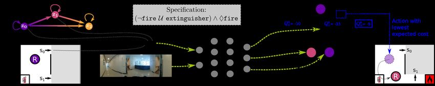
Fig. 4. A comparison between our planner and the baseline for 500 simulated trials in the Firefighting environment with the specification
(¬fire U alarm) ∨ ((¬fire U extinguisher) ∧ ♦fire). The robot (“R”) learns to associate green tiling with the alarm, and hallways emanating
white smoke with fire (A), leading to a 15% improvement for total net cost for this task (B). Our agent learns it is often advantageous to search for the
alarm (C), so in cases where the alarm is reachable, we generally outperform the baseline (highlighted by the cluster of points in the lower half of B). Our
method is occasionally outperformed when the alarm can’t be reached (D), though we perform better in the aggregate and always satisfy the specification.
online execution as needed on a real robot. Once our agent through 5 fully connected layers, and the network outputs the
has searched for the action with lowest expected cost, a∗sz0 z00 , properties required for Eq. (3)—PS , RS , and RF . We train
it generates a motion plan through space to the subgoal our network with the same loss function as in [23].
associated with the chosen action. While moving along this To collect training data, we navigate through environments
path, the agent receives new observations of the world, using an autonomous, heuristic-driven agent in simulation,
updates its map, and replans (see Fig. 1 and Algorithm 1). and teleoperation in the real world. We assume the agent
has knowledge of propositions in its environments, so it can
IV. L EARNING T RANSITION P ROBABILITIES AND C OSTS generate the feature vectors that encode actions for subgoals
To plan with our high-level actions, we rely on values it encounters. As the robot travels, we periodically collect
for PS , RS , and RF for arbitrary actions asz0 z00 . Computing images and the true values of PS (either 0 or 1), RS , and
these values explicitly from the belief (as defined in Sec. III- RF for each potential action from the underlying map.
A) is intractable, so we train a neural network to estimate
them from visual input and an encoding of the action. V. E XPERIMENTS
We perform experiments in simulated and real-world en-
A. Encoding a Transition vironments, comparing our approach with a baseline derived
A successful action asz0 z00 results in the desired transition from Ayala et al. [13]. The baseline solves similar planning-
in the DFA from z 0 to z 00 occurring in unknown space. How- under-uncertainty problems using boundaries between free
ever, encoding actions directly using DFA states prevents and unknown space to define actions, albeit with a non-
our network from generalizing to other specifications with- learned selection procedure and no visual input. Specifically,
out retraining. Instead, we use an encoding that represents we compare the total distances traveled using each method.
formulas over the set of propositions Σ in negative normal
form [27] over the truth values of Σ, which generalizes to A. Firefighting Scenario Results
any specification written with Σ in similar environments. Our first environment is based on the firefighting robot
To progress from z 0 to z 00 in unknown space, the robot example, simulated with the Unity game engine [28] and
must travel such that it remains in z 0 until it realizes shown in Fig. 4. The robot is randomly positioned in one of
changes in proposition values that allow it to transition two rooms, and the extinguisher and exit in the other. One of
to z 00 . We therefore define two n-element feature vectors three hallways connecting the rooms is randomly chosen to
[φ(z 0 , z 0 ), φ(z 0 , z 00 )] where φ ∈ {−1, 0, 1}n , which serve as be a dead end with an alarm at the end of it, and is visually
input to our neural network. For the agent to stay in z 0 , if the highlighted by a green tiled floor. A hallway (possibly the
ith element in φ(z 0 , z 0 ) is 1, the corresponding proposition same one) is chosen at random to contain a fire, which blocks
must be true at all times; if it is −1, the proposition must passage and emanates white smoke. Our network learns to
be false; and if it is 0, the proposition has no effect on
the desired transition. The values in φ(z 0 , z 00 ) are defined
similarly for the agent to transition from z 0 to z 00 . Fig. 3
illustrates this feature vector for a task specification example.
B. Network Architecture and Training
Our network takes as input a 128×512 RGB panoramic
image centered on a subgoal, the scalar distance to that
subgoal, and the two n-element feature vectors φ describing
the transition of interest, as defined in Sec. IV-A. The input
image is first passed through 4 convolutional layers, after
which we concatenate the feature vectors and the distance Fig. 5. A) Visual scenes from our Delivery scenario in simulation. The
to the subgoal to each element (augmenting the number of rooms which can contain professors, graduate students, and undergraduates
are colored differently and illuminated when occupied. B) A comparison
channels accordingly), and continue encoding for 8 more between our approach (left) and the baseline (right) for one of several
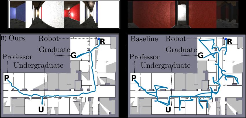
convolutional layers. Finally, the encoded features are passed simulated trials for the task ♦professor ∧ ♦grad ∧ ♦undergrad.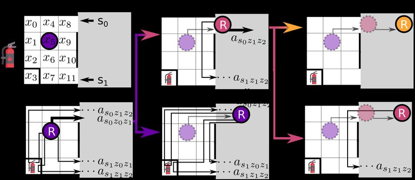
Fig. 6. A comparison between our approach (A-D) and the baseline (E) for our real-world Delivery scenario. Our agent (blue dot) correctly predicts
actions likely to fail (e.g., dark rooms in A) and succeed (e.g., completing a delivery in an illuminated room in B). Once the robot identifies delivery
actions that lead to DFA transitions in known space, it executes them (C-D). Conversely, the baseline fully explores space before completing the task (E).

associate the visual signals of green tiles and smoke to the                   C. Delivery Scenario Results in the Real World
hallways containing the alarm and the fire, respectively.                         We extend our Delivery scenario to the real world using
  We run four different task specifications—using the same                     a Toyota Human Support Robot (HSR) [29] with a head-
network without retraining to demonstrate its reusability:                     mounted panoramic camera [30] in environments with mul-
  1) (¬fire U alarm) ∨ ((¬fire U extinguisher) ∧                               tiple rooms connected by a hallway. The robot must deliver
     ♦fire): avoid the fire until the alarm is found, or avoid                 a package and a document to two people, either unordered
     the fire until the extinguisher is found, then find the fire.             (♦DeliverDocument ∧ ♦DeliverPackage) or in or-
  2) ¬fire U (alarm ∧ ♦exit): avoid the fire until the                         der (♦(DeliverDocument ∧ ♦DeliverPackage)). As
     alarm is found, then exit the building.                                   in simulation, rooms are illuminated only if occupied.
  3) (¬fire U extinguisher) ∧ ♦(fire ∧ ♦exit):                                    We ran 5 trials for each planner spanning both specifica-
     avoid the fire until the extinguisher is found, then put                  tions and 3 different target positions in a test environment
     out the fire and exit the building.                                       different from the one used to collect training data. We show
                                                                               improved performance over the baseline in all cases with a
  4) ¬fire U exit: avoid the fire and exit the building.
                                                                               mean per-trial cost improvement of 36.6% (6.2% standard
   Over ∼3000 trials across different simulated environments                   error), and net cost savings, summed over all trials, of 36.5%.
and these four specifications, we demonstrate improvement                      As shown in Fig. 6, the baseline enters the nearest room
for our planner over the baseline (see Table I). Fig. 4 gives                  regardless of external signal, while our approach prioritizes
a more in depth analysis of the results for specification 1.                   illuminated rooms, which are more likely to contain people.
                            TABLE I                                                                   VI. R ELATED W ORKS
                 Average Cost          Percent Savings
    Spec Known Map Baseline Ours Net Cost Per Trial (S.E.)                        Temporal logic synthesis has been used to generate prov-
     1      187.0      264.6   226.9 15%      14.4% (1.3)                      ably correct controllers, although predominantly in fully
     2      392.1      696.0   461.2 34%      28.4% (1.0)
     3      364.3      539.3   471.3 13%      6.1% (1.3)
                                                                               known environments [2–6]. Recent work has looked at satis-
     4      171.2      269.1   203.3 25%      14.6% (1.0)                      fying LTL specifications under uncertainty beyond LOMDPs
                                                                               [11, 12], yet these works are restricted to small state spaces
                                                                               due to the general nature of the POMDPs they handle. Other
B. Delivery Scenario Results in Simulation                                     work has explored more restricted sources of uncertainty,
                                                                               such as scenarios where tasks specified in LTL need to
   We scale our approach to larger simulated environments                      be completed in partially explored environments [13–17]
using a corpus of academic buildings containing labs,                          or by robots with uncertainty in sensing, actuation, or the
classrooms, and offices, all connected by hallways. Our                        location of other agents [31–34]. When these robots plan in
agent must deliver packages to three randomly placed in-                       partially explored environments, they take the best possible
dividuals in these environments: one each of a professor,                      action given the known map, but either ignore or make
graduate student, and undergraduate, using the specification                   naive assumptions about unknown space; conversely, we use
♦professor ∧ ♦grad ∧ ♦undergrad. Professors are                                learning to incorporate information about unexplored space.
located randomly in offices, graduate students in labs, and                       To minimize the cost of satisfying LTL specifications,
undergraduates in classrooms, which have differently colored                   other recent works have used learning-based approaches [18,
walls in simulation. Rooms that are occupied have the lights                   20, 21, 36], yet these methods are limited to relatively small,
on whereas other rooms are not illuminated.                                    fully observable environments. Sadigh et al. [19] and Fu
   Our agent is able to learn from these visual cues to                        and Topcu [20] apply learning to unknown environments and
navigate more efficiently. Over 80 simulations across 10                       learn the transition matrices for MDPs built from LTL speci-
environments, the mean per-trial cost improvement of our                       fications. However, these learned models do not generalize to
agent compared with the baseline is 13.5% (with 6.1%                           new specifications and are demonstrated on relatively small
standard error). Our net cost savings, summed over all trials,                 grid worlds. Paxton et al. [22] introduce uncertainty during
is 7.8%. Fig. 5 illustrates our results.                                       planning, but limit their planning horizon to 10 seconds,
which is insufficient for the specifications explored here. Carr [15] M. Guo and D. V. Dimarogonas. “Multi-agent plan reconfiguration
et al. [37] synthesize a controller for verifiable planning in under local LTL specifications”. In: IJRR 34.2 (2015).
[16] M. Lahijanian et al. “Iterative Temporal Planning in Uncertain
POMDPs using a recurrent neural network, yet are limited Environments With Partial Satisfaction Guarantees”. In: TRO (2016).
to planning in small grid worlds. [17] S. Sarid et al. “Guaranteeing High-Level Behaviors While Exploring
Partially Known Maps”. In: RSS. 2012.
VII. C ONCLUSION AND F UTURE W ORK [18] R. Toro Icarte et al. “Teaching Multiple Tasks to an RL Agent Using
LTL”. In: AAMAS. 2018.
In this work, we present a novel approach to planning [19] D. Sadigh et al. “A learning based approach to control synthesis of
to solve scLTL tasks in partially revealed environments. Our markov decision processes for linear temporal logic specifications”.
In: CDC. 2014.
approach learns from raw sensor information and generalizes [20] J. Fu and U. Topcu. “Probably Approximately Correct MDP Learning
to new environments and task specifications without the need and Control With Temporal Logic Constraints”. In: RSS. 2015.
to retrain. We hope to extend our methods to real-world [21] M. L. Littman et al. “Environment-independent task specifications
via GLTL”. In: arXiv (2017).
planning domains that involve manipulation and navigation. [22] C. Paxton et al. “Combining neural networks and tree search for task
and motion planning in challenging environments”. In: IROS. 2017.
R EFERENCES [23] G. J. Stein et al. “Learning over Subgoals for Efficient Navigation
[1] A. Duret-Lutz et al. “Spot 2.0 — a framework for LTL and ω- of Structured, Unknown Environments”. In: CoRL. 2018.
automata manipulation”. In: ATVA. Springer, 2016. [24] O. Kupferman and M. Y. Vardi. “Model checking of safety proper-
[2] H. Kress-Gazit et al. “Synthesis for Robots: Guarantees and Feed- ties”. In: Formal Methods in System Design. 2001.
back for Robot Behavior”. In: Annual Review of Control, Robotics, [25] D. Silver and J. Veness. “Monte-Carlo Planning in Large POMDPs”.
and Autonomous Systems (2018). In: Advances in Neural Information Processing Systems. 2010.
[3] G. E. Fainekos et al. “Temporal logic motion planning for dynamic [26] J. Pineau and S. Thrun. An integrated approach to hierarchy and
robots”. In: Automatica (2009). abstraction for POMDPs. Tech. rep. CMU, 2002.
[4] A. Bhatia et al. “Sampling-based motion planning with temporal [27] J. Li et al. “On the Relationship between LTL Normal Forms
goals”. In: ICRA. 2010. and Büchi Automata”. In: Theories of Programming and Formal
[5] B. Lacerda et al. “Optimal and dynamic planning for Markov Methods. 2013.
decision processes with co-safe LTL specifications”. In: IROS. 2014. [28] Unity Technologies. Unity Game Engine. unity3d.com. 2019.
[6] S. L. Smith et al. “Optimal path planning for surveillance with [29] T. Yamamoto et al. “Development of HSR as the research platform
temporal-logic constraints”. In: IJRR 30.14 (2011). of a domestic mobile manipulator”. In: ROBOMECH (2019).
[7] M. Merlin et al. “Locally Observable Markov Decision Processes”. [30] Ricoh Theta S Panoramic Camera. 2019.
In: ICRA 2020 Workshop on Perception, Action, Learning. 2020. [31] C.-I. Vasile et al. “Control in Belief Space with Temporal Logic
[8] L. P. Kaelbling et al. “Planning and Acting in Partially Observable Specifications”. In: CDC. 2016.
Stochastic Domains”. In: Artificial Intelligence (1998). [32] Y. Kantaros et al. “Reactive Temporal Logic Planning for Multiple
[9] M. L. Littman et al. “Learning policies for partially observable Robots in Unknown Environments”. In: ICRA. 2020.
environments: Scaling up”. In: Machine Learning Proceedings. 1995. [33] Y. Kantaros and G. Pappas. “Optimal Temporal Logic Planning for
[10] O. Madani. “On the Computability of Infinite-Horizon Partially Multi-Robot Systems in Uncertain Semantic Maps”. In: IROS. 2019.
Observable Markov Decision Processes”. In: AAAI (1999). [34] M. Svoreňová et al. “Temporal logic motion planning using POMDPs
[11] M. Bouton et al. “Point-Based Methods for Model Checking in with parity objectives: case study paper”. In: HSCC. 2015.
Partially Observable Markov Decision Processes.” In: AAAI. 2020. [35] K. Horák and B. Bošanskỳ. “Solving Partially Observable Stochastic
[12] M. Ahmadi et al. “Stochastic finite state control of POMDPs with Games with Public Observations”. In: AAAI. 2019.
LTL specifications”. In: arXiv (2020). [36] X. Li et al. “A formal methods approach to interpretable reinforce-
[13] A. I. M. Ayala et al. “Temporal logic motion planning in unknown ment learning for robotic planning”. In: Science Robotics (2019).
environments”. In: IROS. 2013. [37] S. Carr et al. “Verifiable RNN-Based Policies for POMDPs Under
[14] M. Guo et al. “Revising Motion Planning Under Linear Temporal Temporal Logic Constraints”. In: IJCAI. 2020.
Logic Specifications in Partially Known Workspaces”. In: ICRA.
2013.You can also read