Boosting Offline Reinforcement Learning with Residual Generative Modeling
←
→
Page content transcription
If your browser does not render page correctly, please read the page content below

Boosting Offline Reinforcement Learning with Residual Generative Modeling
                                                               Hua Wei1 , Deheng Ye1 , Zhao Liu1 , Hao Wu1 , Bo Yuan1 ,
                                                                      Qiang Fu1 , Wei Yang1 and Zhenhui (Jessie) Li 2
                                                                               1
                                                                                 Tencent AI Lab, Shenzhen, China
                                                                  2
                                                                    The Pennsylvania State University, University Park, USA
                                                     {harriswei, dericye, ricardoliu, alberthwu, jerryyuan, leonfu, willyang}@tencent.com
                                                                                       jessieli@ist.psu.edu
arXiv:2106.10411v2 [cs.LG] 22 Jun 2021

                                                                   Abstract                                  of Kings) that require highly complex action control, cur-
                                                                                                             rent RL methods still learn from the scratch, resulting in a
                                              Offline reinforcement learning (RL) tries to learn             long time to master human-level skills [Berner et al., 2019;
                                              the near-optimal policy with recorded offline ex-              Ye et al., 2020c], where there is a large amount of logged
                                              perience without online exploration. Current of-               replay data from vast players to be utilized.
                                              fline RL research includes: 1) generative modeling,
                                              i.e., approximating a policy using fixed data; and                Although off-policy RL methods [Mnih et al., 2015; Lill-
                                              2) learning the state-action value function. While             icrap et al., 2015; Haarnoja et al., 2018] may be executed in
                                              most research focuses on the state-action func-                the offline scenario directly, their performance was shown to
                                              tion part through reducing the bootstrapping er-               be poor [Fujimoto et al., 2019] with a fixed batch of data and
                                              ror in value function approximation induced by                 no interactions with the environment. The poor performance
                                              the distribution shift of training data, the effects           is suspected due to incorrect value estimation of actions out-
                                              of error propagation in generative modeling have               side the training data distribution [Kumar et al., 2019]. The
                                              been neglected. In this paper, we analyze the                  error of estimated values will accumulate and amplify dur-
                                              error in generative modeling. We propose AQL                   ing the Bellman backup process in RL. Typical off-policy RL
                                              (action-conditioned Q-learning), a residual gener-             would improve the learned policy by trying out the policy in
                                              ative model to reduce policy approximation error               the environment to correct the erroneous estimations, which
                                              for offline RL. We show that our method can learn              is not applicable in purely offline scenarios.
                                              more accurate policy approximations in different                  Instead of correcting erroneous estimations by interact-
                                              benchmark datasets. In addition, we show that the              ing with the environment, offline RL provides an alterna-
                                              proposed offline RL method can learn more com-                 tive for the offline scenario. Current representative offline
                                              petitive AI agents in complex control tasks under              RL methods [Fujimoto et al., 2019; Kumar et al., 2019;
                                              the multiplayer online battle arena (MOBA) game                Wu et al., 2019; Kumar et al., 2020] mainly study how to
                                              Honor of Kings.                                                reduce the error with conservative estimations, i.e., constrain-
                                                                                                             ing the action or state-action distribution around the given
                                                                                                             dataset’s distribution when learning value functions. With
                                         1   Introduction                                                    such estimations, the learned RL policy can approach or ex-
                                         Reinforcement learning (RL) has achieved promising results          ceed the original policy (also called behavioral policy) that
                                         in many domains [Mnih et al., 2015; Silver et al., 2017;            generates the fixed dataset. As most offline RL methods as-
                                         Kalashnikov et al., 2018; Berner et al., 2019; Vinyals et al.,      sume that the behavioral policy is unknown, typical offline
                                         2019; Ye et al., 2020b; Ye et al., 2020a]. However, be-             RL methods would first approximate the behavioral policy
                                         ing fettered by the online and trial-and-error nature, apply-       through generative modeling [Levine et al., 2020], i.e., learn
                                         ing RL in real-world cases is difficult [Dulac-Arnold et al.,       to output actions for given states. Then, the objective is to
                                         2019]. Unlike supervised learning which directly benefits           learn approximations for selecting the highest valued actions
                                         from large offline datasets like ImageNet [Deng et al., 2009],      that are similar to the approximated behavioral policy.
                                         current RL has not made full use of offline data [Levine et            Different from the aforementioned methods, this paper fo-
                                         al., 2020]. In many real-world scenarios, online exploration        cuses on investigating the impact of errors from generative
                                         of the environment may be unsafe or expensive. For exam-            modeling on offline RL. As we will show, in value-based off-
                                         ple, in recommendation [Li et al., 2011] or healthcare do-          policy scenarios, the error of generative modeling will accu-
                                         mains [Gottesman et al., 2019], a new policy may only be            mulate in the process of learning the Q-value function during
                                         deployed at a low frequency after extensive testing. In these       Bellman backup. Our main contribution involves studying the
                                         cases, the offline dataset is often large, potentially consist-     accumulating process of generative modeling error in offline
                                         ing of years of logged experiences. Even in applications            RL and developing a practical method to mitigate this error.
                                         where online exploration is feasible, offline data is still bene-   To expand, we first examine the error accumulation process
                                         ficial. For example, in strategy video games (Dota or Honor         during offline RL learning in detail and analyze the influence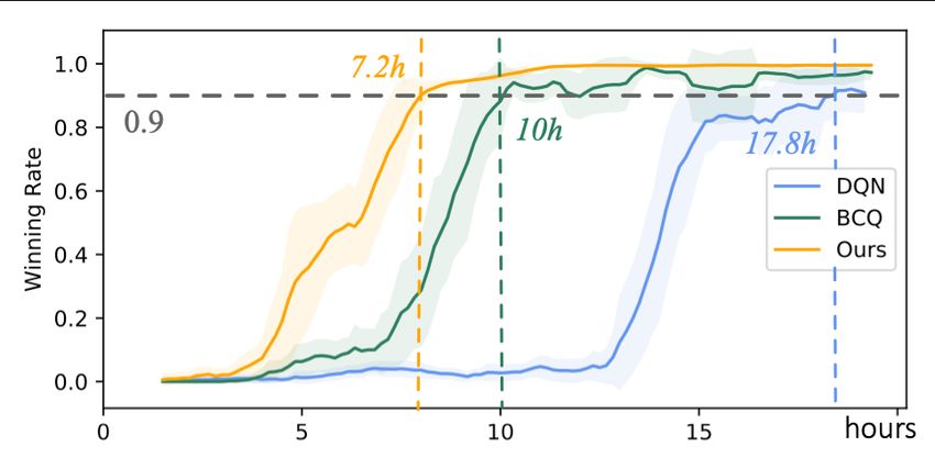
of generative modeling error on the final offline RL error on            3.2     Offline Reinforcement Learning
the Q-value function. Then we propose an error reduction                 Offline RL additionally considers the problem of learning
method via residual learning [Huang et al., 2017]. Through               policy π from a fixed dataset D consisting of single-step tran-
experiments on a set of benchmark datasets, we verify the ef-            sitions (st , at , rt , st+1 ), without interactions with the environ-
fectiveness of our method in boosting offline RL performance             ment. This is in contrast to many off-policy RL algorithms
over state-of-the-art methods. Furthermore, in the scenario of           that assume further interactions with the current policy rolling
the multiplayer online battle arena (MOBA) game Honor of                 out in the environment. In this paper, we define the behavioral
Kings, which involves large state-action space, our proposed             policy πb as the conditional distribution p(a|s) in the dataset
method can also achieve excellent performance.                           D, which is treated unknown. In real-world cases, the train-
                                                                         ing dataset could be generated by a collection of policies. For
2     Related Work                                                       simplicity, we refer to them as a single behavioral policy πb .
Under fully offline settings where no additional online data             Value Function Approximation
collection is performed, both offline RL methods and imi-                For large or continuous state and action spaces, the value
tation learning methods can be used to learn a policy from               function can be approximated with neural networks Q̂θ , pa-
pre-recorded trajectories.                                               rameterized by θ. With the notion of Bellman operator T π ,
Offline RL. Offline RL describes the setting in which a                  we can denote Equation (1) as Q̂π = T π Q̂π with γ ∈ [0, 1).
learner has access to only a fixed dataset of experience, in             This Bellman operator has a unique fixed point that corre-
contrast to online RL which allows interactions with the envi-           sponds to the true state-value function for π(a|s), which can
ronment. Existing offline RL methods suffer from issues per-             be obtained by repeating the iteration Q̂πk+1 = Tkπ Q̂π , and it
taining to OOD actions [Fujimoto et al., 2019; Kumar et al.,
2019; Wu et al., 2019; Kumar et al., 2020]. Prior works aim              can be shown that limk→∞ Q̂πk = T π Q̂π .
to make conservative value function estimations around the                  Offline RL algorithms based on this value function ap-
given dataset’s distribution, and then only use action sampled           proximation with the iterative update are shown to suf-
from this constrained policy in Bellman backups for applying             fer from action distribution shift [Fujimoto et al., 2019]
value penalty. Different from these works, this paper focuses            during training.       Since the policy in next iterate is
on how the errors propagate throughout the whole process of              computed by choosing actions that greedily maximize
offline RL, from generative modeling to value approximation.             the state-action value function at each state, πk+1 (a|s) =
                                                                         arg maxa Qπk (s, a), it may be biased towards out-of-
Imitation learning. Imitation learning (IL) is to learn be-              distribution (OOD) actions with erroneously high Q-values.
havior policies from demonstration data [Schaal, 1999; Hus-              In RL with explorations, such errors can be corrected by
sein et al., 2017]. Though effective, these methods are not              rolling out the action in the environment and observing its
suitable for offline RL setting because they require either on-          true value. In contrast, an offline RL agent is unable to query
policy data collection or oracle policy. Different from offline          such information from the environment. To mitigate the prob-
RL, imitation learning methods do not necessarily consider               lem caused by OOD actions, typical offline RL methods focus
modeling the long-term values of actions or states like rein-            on constraining the learned policy to output actions that lie in
forcement learning methods.                                              the training distribution πb .

3     Preliminaries                                                      Generative Modeling
                                                                         Because we do not assume direct access to πb , it is common
3.1     Reinforcement Learning                                           in previous work to approximate this behavior policy via a
We consider the environment as a Markov Decision Process                 generative model Gω (s), with max-likelihood over D [Fu-
(MDP) (S, A, P, R, γ), where S is the state space, A is the              jimoto et al., 2019; Kumar et al., 2019; Wu et al., 2019;
action space, P : S × A × S → [0, 1] denotes the state                   Levine et al., 2020]:
transition probability, R : S × A → R represents the reward
function, and γ ∈ (0, 1] is the discount factor. A policy π is a               Gω (s) = π̂b := arg max E(s,a,r ,s 0 )∼D [log π̂(a|s)]      (2)
mapping S × A → [0, 1].                                                                               π̂
   A value function provides an estimate of the expected cu-                We denote the approximated policy as πˆb and refer to it as
mulative reward that will be obtained by following some pol-             “cloned policy” to distinguish it from πb .
icy π(at |st ) when starting from a state-action tuple (st , at ) in        In Section 4, we will analyze how the errors propagate
the case of the state-action value function Qπ (st , at ):               from generative modeling to value function approximation,
                                                                         resulting in the overall errors for offline RL. Then we will in-
                                                                         troduce how to reduce the overall errors of offline RL by re-
    Qπ (st , at ) = r(st , at ) + γEst+1 ,at [Qπ (st+1 , at+1 )]   (1)   ducing the generative modeling error, with theoretical proofs
   In the classic off-policy setting, the learning of Q-function         and implemented models in Section 5.
is based on the agent’s replay buffer D that gathers the ex-
perience of the agent in the form of (st , at , rt , st+1 ), and         4     Generative Modeling Error Propagation
each new policy πk collects additional data by exploring the             In this section, we define and analyze how the generative
environment. Then D, which consists of the samples from                  modeling error propagates during the process of value esti-
π0 , . . . , πk , is used to train a new updated policy πk+1 .           mation in offline RL. We derive bounds which depend on the
generative modeling. This motivates further focusing on mit- The proof follows by expanding each Q, rearranging terms,
igating generative modeling error. simplifying the expression and then representing cloned pol-
icy π with behavior policy πb with a generative error g .
4.1 Generative Modeling Error Based on above equation, we take the supremum of
As discussed in the last section, we need to approximate πD (s, a) and have the following:
πD (s, a) with a generative model Gω (s). If we train Gω (s)
with supervised learning (i.e., standard likelihood maximiza- X
sup πD (s, a) ≥ (p∗ (s0 |s, a) − pD (s0 |s, a))
tion) on D, we have the following result from [Ross et al., D
s0
2011], whose proof can be found in [Levine et al., 2020]. X
Lemma 1 (Behavioral cloning error bound). If τ (s) is the πb · [r(s, a) + γ( (πb (a0 |s0 ) + |A|η)QπD (s0 , a0 )] (6)
a0
state distribution induced by πb and π(a|s) is trained via X
standard likelihood maximization on s ∼ τ πb (s) and optimal + p∗ (s0 |s, a) · γ( πb (a0 |s0 ) + |A|η)πD (s, a)
labels a, and attains generalization error g on s ∼ τ πb (s), a0
then l (π) ≤ C + H 2 g is the best possible bound on the
expected error of the learned policy, where C is the true ac-
cumulated reward of πb . For a finite, deterministic MDP, if all possible state tran-
This means that even with optimal action labels, we still sitions are captured in D, pD (s0 |s, a) will be equivalent to
get an error bound at least quadratic in the time horizon H in p∗ (s0 |s, a), we will have πD (s, a) = 0. However, in infinite
the offline case. Intuitively, the policy π̂b learned with gener- or stochastic MDP, it might require an infinite number of sam-
ative model Gω (s) may enter into states that are far outside of ples to cover the true distribution. Therefore, δ(s, a) = 0 if
the training distribution, where the generalization error bound and only if the following strong assumptions holds: the true
g no longer holds on unseen states during training. Once the MDP is finite and deterministic, and all possible state transi-
policy enters one OOD state, it will keep making mistakes tions are captured in D. Otherwise, we have δ(s, a) > 0.
and remain OOD for the remainder of the testing phase, ac- From Theorem 1, we have δ(s, a) scales as O(η|A|), where
cumulating O(H) error. Since there is a non-trivial chance of η(s, a) = supD g (a|s). Intuitively, this means we can
entering an OOD state at every one of the H steps, the overall prevent an increase in the state-action value function error
error scales as O(H 2 ). by learning a generative model Gω (s) with smaller g .
Meanwhile, for settings where the action space is small,
4.2 Error Propagation on Value Estimation the g are will have smaller influences in inducing the
Definition 1 (Value function approximation error). We de- state-action value function error. Overall, in the time horizon
fine πD (s, a) as the value function approximation error be- H, since the generative error g scales as O(H 2 ), δ(s, a) =
tween the true state-action value function QπD computed from supD πD (s, a) scales as O(|A|H 2 ).
the dataset D and the true state-action value function Q∗ :
5 Residual Generative Modeling
πD (s, a) = Q∗ (s, a) − QπD (s, a) (3) We begin by analyzing the theoretical properties of residual
Theorem 1. Given a policy πb that generates the dataset D, generative modeling in a deterministic policy setting, where
if we model its cloned policy π̂b from D with a generative we are able to measure the monotonically decreasing loss
modeling error of g , assume that δ(s, a) = supD πD (s, a) over sampled actions precisely. We then introduce our deep
and η(s, a) = supD g (a|s), with the action space of dimen- reinforcement learning model in detail, by drawing inspira-
sion |A|, δ(s, a) satisfies the following: tions from the deterministic analog.
X
δ(s, a) ≥ (p∗ (s0 |s, a) − pD (s0 |s, a)) 5.1 Addressing Generative Modeling Error with
s0 Residual Learning
X
· [r(s, a) + γ( (πb (a0 |s0 ) + |A|η)QπD (s0 , a0 )] In this section, we will provide a short theoretical illustration
(4) of how residual learning can be used in addressing the gener-
a0
∗ 0
X ative modeling under deterministic policies. In this example,
+ p (s |s, a) · γ( πb (a0 |s0 ) + |A|η)πD (s, a) we will assume that ρφ (s) is the original generative model in
a0 mimicking the policy πb in dataset D, and the residual gener-
Proof. Firstly, we have the following: ative model is denoted as â = Gω (s, ρφ (s)), where ω stands
for the parameters used to combine input s and generative
model ρφ (s).
X
πD (s, a) = (p∗ (s0 |s, a) − pD (s0 |s, a))
s0
Without loss of generality, we can re-write the final out-
X put layer by assuming that Gω is parameterized by a linear
· [r(s, a) + γ (πb (a0 |s0 ) + g (a0 |s0 ))QπD (s0 , a0 )] (5) weight vector w and a weight matrix M, and previous lay-
a0 ers can be represented as Gω2 (s). Thus, â can be denoted as
â = wT (MGω2 (s) + ρφ (s)). We have the following result
X
+ p∗ (s0 |s, a) · γ (πb (a0 |s0 ) + g (a0 |s0 ))πD (s0 , a0 )
a0
from [Shamir, 2018]:Lemma 2. Suppose we have a function defined as and outputs the reconstructed action. The overall training loss
. . for the conditional VAE is:
Γψ (a, B) = Γ(a, B, ψ) = Ex,y l aT (H(x) + BFψ (x) , y
(7) LV AE = −Ez∼q(z|s,a) [log p(a|s, z)]+DKL (q(z|s, a)||p(z))
where l is the defined loss, a, B are weight vector and matrix (10)
respectively, and ψ is the parameters of a neural network. where the first term is the reconstructed loss, and the second
Then, every local minimum of Γ satisfies term is the regularizer that constrains the latent space distri-
bution, s is the state input to the conditional VAE, a is the
Γ(a, B, ψ) ≤ inf Γ(a, 0, ψ) (8) action in the dataset in pair with s.
a
if following conditions are satisfied: (1) loss l(ŷ, y) is twice Residual Network
differentiable and convex in ŷ; (2) Γψ (a, B), 5Γψ (a, B), Unlike BCQ and BEAR which take VAE or a single feed-
and 52 Γψ (a, B) are Lipschitz continuous in (a, B). forward neural network as the generative model, we propose
to use the reconstructed action from VAE as an additional
Theorem 2. When using log loss or squared loss for deter- input to learn the residual of action output. This residual
ministic policy and linear or convolution layers for Fω2 , ev- mechanism is motivated to boost offline RL by reducing the
ery local optimum of â = wT (MGω2 (s) + ρφ (s)) will be no generative model’s error. The overall loss for the generative
worse than â = wT ρφ (s) . network is:
Proof. For deterministic policies, Gω2 (x) is Lipschitz con-
tinuous when using linear or convolution layers [Virmaux and Lω = Eω [d(â, a)] + LV AE (11)
Scaman, 2018]. Since log loss and squared loss are twice dif- where â = Gω (s) is the output of the residual network, and
ferentiable in a, we have d(â, a) is the distance measure between two actions. For con-
tinuous actions, d could be defined as the mean squared error;
Γ(w, M, θ) ≤ infw Γ(w, 0, θ) (9) for discrete actions, d could be defined as the cross-entropy.
. T Intuitively, this loss function includes the original generative
where Γψ (a, B) = Γ(a, B, ψ) = Ex,y [l(a (H(x) +
BFθ (x)), y)], l is the defined loss, a , B are weight vector modeling loss function (usually treated the same as a behav-
and matrix respectively, and θ is the parameters of a neural ior cloning loss) and a VAE loss, optimized at the same time.
network.
5.3 Training Process
That is, the action-conditioned model has no spurious local
minimum that is above that of the original generative model We now describe the practical offline RL method based on
ρφ (s). BEAR , a similar variant on BCQ or other methods can be
similarly derived. Empirically we find that our method based
5.2 Residual Generative Model on BEAR performs better. We’ve described our generative
The main difference between our method and existing offline model in previous sections, here we briefly introduce the
RL methods is that we design a residual modeling part for the other part of the offline RL algorithm, i.e., value function ap-
generative model when approximating the πD . Therefore, in proximation process, which is similar to BCQ and BEAR .
this section, we mainly introduce our approach to offline re- To compute the target Q-value for policy improvement, we
inforcement learning, AQL (action-conditioned Q-learning), use the weighted combination of the maximum and the mini-
which uses action-conditioned residual modeling to reduce mum Q-value of K state-action value functions, which is also
the generative modeling error. adopted in BCQ and BEAR and shown to be useful to penal-
Our generative model consists of two major components: ize uncertainty over future states in existing literature [Fuji-
a conditional variational auto-encoder (VAE) that models the moto et al., 2019]:
distribution by transforming an underlying latent space, and y(s, a) = r + γ max[λ min Qθj0 (s0 , ai )
ai j=1,...,K
a residual neural network that models the state-action distri- (12)
bution residuals on the output of the VAE. + (1 − λ) max Qθj0 (s 0 , ai )]
j=1,...,K
Conditional VAE
where s0 is the next state of current state s after taking action
To model the generative process of predicting actions given a, θj0 is the parameters for target network, γ is the discount
certain states, analogous to existing literatures like Batch- factor in Bellman Equation, λ is the weighting factor.
Constrained Q-learning (BCQ ) [Fujimoto et al., 2019] and Following BEAR , we define the generative modeling up-
Bootstrapping error reduction (BEAR ) [Kumar et al., 2019], date process as a constrained optimization problem, which
we use a conditional VAE that takes state and action as in- tries to improve the generator and constrains the policy within
put and outputs the reconstructed action. Given the raw state, a threshold :
we first embed the state observation with a state embedding
module in conditional VAE. Then in the encoder part, we
concatenate the state embedding with action input and out- Gω = max E(s,a,r,s0 )∼D [Eâ∼Gω (s) min Qi (s, â)
Gω i=1,...,K
put the distribution of latent space (assumed to be Gaussian (13)
− α(LGω (s) − )]
for continuous action space and Categorical for discrete ac-
tion space). In the decoder part, we concatenate the state em- where α is the tradeoff factor that balances constraining the
bedding and the latent variable z from the learned distribution policy to the dataset and optimizing the policy value, and canbe automatically tuned via Lagrangian dual gradient descent Figure 1 shows the comparison of the error, with the mean
for continuous control and is fixed as a constant for discrete and standard deviation from the last 500 training batches of
control. each method. We have the following observations:
This forms our proposed offline RL method, which consists • Both AQL and BEAR have a lower error in generative mod-
of three main parameterized components: a generative model eling than BCQ , and both AQL and BEAR keep the errors
Gω (s), Q-ensemble {Qθi }K K
i=1 , target Q-networks {Qθi0 }i=1 below 0.05 in most cases. This is because they use the dual
and target generative model Gω0 . In the following section, we gradient descent to keep the target policy constrained below
demonstrate AQL results in mitigating the generative model- the threshold that is set as 0.05, while BCQ does not have
ing error and a strong performance in the offline RL setting. this constraint.
• Our proposed method AQL has a consistent lower error
6 Experiment than BEAR . This is because AQL uses residual learning to
mitigate the generative modeling error, which matches our
We compare AQL to behavior cloning, off-policy methods analysis, as suggested by Theorem 2.
and prior offline RL methods on a range of dataset composi- Effectiveness of boosting offline RL. As analyzed in
tions generated by (1) completely random behavior policy, (2) previous sections, we can prevent an increase in the
partially trained, medium scoring policy, and (3) an optimal state-action value function error by learning a generative
policy. Following [Fujimoto et al., 2019; Kumar et al., 2019; model Gω (s) with smaller g , and thus learn a better offline
Wu et al., 2019], we evaluate performance on four Mu- RL policy. Here, we investigate the effectiveness of the pro-
joco [Todorov et al., 2012] continuous control environments posed method on boosting the performance of offline RL.
in OpenAI Gym [Brockman et al., 2016]: HalfCheetah-v2, Table 1 shows the comparison of our proposed method over
Hopper-v2, and Walker2d-v2. We evaluate offline RL algo- behavior cloning, off-policy methods, and state-of-the-art of-
rithms by training on these fixed datasets provided by open- fline RL methods. We have the following observations:
access benchmarking dataset D4RL [Fu et al., 2020] and eval- • Off-policy methods (DDPG and SAC ) training in an purely
uating the learned policies on the real environments. The offline setting yields a bad performance in all cases. This is
statistics for these datasets can be found in [Fu et al., 2020]. due to the incorrect estimation of the value of OOD actions,
Baselines. We compare with off-policy RL methods - Deep which matches the existing literature.
Deterministic Policy Gradient (DDPG ) [Lillicrap et al., • Offline RL methods can outperform BC under datasets gen-
2015] and Soft Actor-Critic (SAC ) [Haarnoja et al., 2018]), erated by the random and medium policy. This is because BC
Behavior Cloning (BC ) [Ross and Bagnell, 2010], and state- simply mimicking the policy behavior from the dataset with-
of-the-art off-policy RL methods, including BCQ [Fujimoto out the guidance of state-action value. Since the dataset D
et al., 2019], BEAR [Kumar et al., 2019], Behavior Regu- is generated by a non-optimal policy, the policy learned by
larized Actor Critic with policy (BRAC-p) or value (BRAC- BC could generate non-optimal actions. This non-optimality
v) regularization [Wu et al., 2019], and Conservative Q- could accumulate as the policy rolls out in the environments.
Learning (CQL (H)) [Kumar et al., 2020]. We use the open- • AQL performs similarly or better than the best prior meth-
source codes provided in corresponding methods and keep ods in most scenarios. We noticed that BRAC and CQL (H)
the same parameters in our proposed method for a fair com- yields better performance in random and medium data than in
parison. expert data. This is because under expert data, the variance
of the state-action distribution in the dataset might be small,
Experimental settings. To keep the same parameter set- and simply mimicking the behavior policy could yield satis-
tings as BCQ and BEAR , we set K = 2 (number of can- factory performance (like BC ). While BRAC and CQL (H)
didate Q-functions), λ = 0.75 (minimum weighting factor), does not have any specific design to reduce the generative
= 0.05 (policy constraint threshold), and B = 1000 (to- error, AQL has a better generative model to mimicking the
tal training steps). We report the average evaluation return distribution of D and thus consistently performs as one of the
over three seeds of the learned algorithm’s policy, in the form best methods cross most settings. As analyzed in previous
of a learning curve as a function of the number of gradient sections, we can lower the error of state-action value estima-
steps taken by the algorithm. The samples collected during tion, thus boost the offline RL performance.
the evaluation process are only used for testing and not used We also noticed that although the overall performance of
for training. AQL is slightly better than CQL (H), since CQL (H) has ad-
ditional constraints that AQL does not consider. We added
6.1 Results the constraints of CQL (H) into AQL and found out that AQL
Effectiveness of mitigating generative modeling error. In can further improve on CQL (H) in all cases, which means the
previous sections, we argued in favor of using the residual effectiveness of boosting offline RL methods by reducing the
generative modeling to decrease the generative modeling er- generative error.
ror. Revisiting the argument, in this section, we investigate
the empirical results on the error between true a at state s 6.2 Case Study: Honor of Kings 1v1
from D and the generated action â from Gω (s). In BCQ , it An open research problem for existing offline RL methods is
uses a vanilla conditional VAE as Gω (s); BEAR use a sim- the lack of evaluations on complex control tasks [Levine et
ple feed-forward neural network. Our proposed method com- al., 2020; Wu et al., 2019] with large action spaces. There-
bines these two models with a residual network. fore, in this paper, we further implement our experiment into80
BCQ BEAR Ours BCQ BEAR Ours BCQ BEAR Ours
60
60 102
MSE (×10 3)
MSE (×10 3)
MSE (×10 3)
40
40 101
20 20
100
0 0
Random Medium Expert Random Medium Expert Random Medium Expert
(a) H OPPER (b) H ALFCHEETAH (b) WALKER 2 D
Figure 1: The average (with standard deviation) of the mean squared error between a ∼ D(s) and â ∼ Gω (s) from generative model. Note
that the y-axis of H ALFCHEETAH is in log scale. The lower, the better. All the results are reported over last 500 training batches. With
residual network, our proposed method can largely reduce the error.
BC SAC DDPG BCQ BEAR BRAC-p BRAC-v CQL (H) AQL
H ALFCHEETAH-random -17.9 3502.0 209.22 -1.3 2831.4 2713.6 3590.1 3902.4 3053.1
H OPPER-random 299.4 347.7 62.13 323.9 349.9 337.5 376.3 340.7 379.2
WALKER 2 D2d-random 73.0 192.0 39.1 228.0 336.3 -7.2 87.4 346.6 350.3
H ALFCHEETAH-medium 4196.4 -808.6 -745.87 4342.67 4159.08 5158.8 5473.8 5236.8 4397.2
WALKER 2 D2d-medium 304.8 44.2 4.63 2441 2717.0 3559.9 3725.8 3487.1 1763.5
H OPPER-medium 923.5 5.7 10.19 1752.4 1674.5 1044.0 990.4 1694.0 1768.1
H ALFCHEETAH-expert 12984.5 -230.6 -649.1 10539.1 13130.1 461.13 -133.5 12189.9 12303.4
H OPPER-expert 3525.4 22.6 48.2 3410.5 3567.4 213.5 119.7 3522.6 3976.4
WALKER 2 D2d-expert 3143.9 -13.8 9.8 3259.2 3025.7 -9.2 0.0 143.3 3253.5
Table 1: Performance of AQL and prior methods on gym domains from D4RL, on the unnormalized return metric, averaged over three random
seeds, with top-3 emphasized. While BCQ , BEAR , BRAC and CQL (H) perform unstably across different scenarios, AQL consistently
performs similarly or better than the best prior methods.
a multiplayer online battle arena (MOBA) game, the 1v1 ver-
sion of Honor of Kings (the most popular and widely studied
MOBA game at present [Ye et al., 2020a; Ye et al., 2020c;
Chen et al., 2020]). Compared with traditional games like
Go or Atari, Honor of Kings 1v1 version has larger state and
action space and more complex control strategies. A detailed
description of the game can be found in [Ye et al., 2020c].
Baselines. Since the action space is discrete, we compare
our method with DQN [Mnih et al., 2013] and the discrete
version of BCQ [Fujimoto et al., 2019] instead of BEAR .
Compared with DQN , BCQ only adds one generative model Figure 2: Winning rate of different methods against behavior-tree-
to learn the distribution of D. For AQL , we add an residual based AI across training time. Our proposed method can learn a
network upon BCQ as the discrete version of our proposed more competitive agent at a faster learning speed.
method. We use the same network parameters and training
parameters for all the baseline methods for a fair comparison.
7 Conclusion
Results. In our experiment, we evaluate the ability of the
agents learned by DQN , BCQ and our method, against the The goal of this work is to study the impact of generative
internal behavior-tree-based AI in the game, as is shown in modeling error in offline reinforcement learning (RL). We
Figure 2. We have the following observations: theoretically and empirically analyze how error propagates
• Offline RL methods (BCQ and our proposed method) from generative modeling to the value function approxima-
largely reduce the convergence time of classical off-policy tion in Bellman backup of off-policy RL. We propose AQL
method DQN . This means the generative modeling of the (action-conditioned Q-learning), a residual generative model
dataset D helps the learning of value function. to reduce policy approximation error. Our experiments sug-
• Our proposed method further outperform BCQ . Compared gest that AQL can help to boost the performance of offline
with BCQ , the discrete version of our method uses the resid- RL methods. Our case study on complex tasks further veri-
ual network in the generative modeling process, which miti- fies that offline RL methods can efficiently learn with faster
gates the error of modeling the distribution of D, and boosts convergence when integrated in the online process with of-
the performance of learned value function. fline learning.References [Li et al., 2011] Lihong Li, Wei Chu, John Langford, and
[Berner et al., 2019] Christopher Berner, Greg Brockman, Xuanhui Wang. Unbiased offline evaluation of contextual-
bandit-based news article recommendation algorithms. In
Brooke Chan, et al. Dota 2 with large scale deep rein-
WSDM, 2011.
forcement learning. arXiv:1912.06680, 2019.
[Lillicrap et al., 2015] Timothy P Lillicrap, Jonathan J Hunt,
[Brockman et al., 2016] Greg Brockman, Vicki Cheung, et al. Continuous control with deep reinforcement learn-
et al. Openai gym. arXiv:1606.01540, 2016. ing. arXiv:1509.02971, 2015.
[Chen et al., 2020] Sheng Chen, Menghui Zhu, Deheng Ye, [Mnih et al., 2013] Volodymyr Mnih, Koray Kavukcuoglu,
Weinan Zhang, Qiang Fu, and Wei Yang. Which heroes et al. Playing Atari with deep reinforcement learning.
to pick? learning to draft in moba games with neural net- arXiv:1312.5602, 2013.
works and tree search. arXiv:2012.10171, 2020.
[Mnih et al., 2015] Volodymyr Mnih, Koray Kavukcuoglu,
[Deng et al., 2009] Jia Deng, Wei Dong, Richard Socher, Li- David Silver, et al. Human-level control through deep re-
Jia Li, Kai Li, and Li Fei-Fei. Imagenet: A large-scale inforcement learning. Nature, 518(7540), 2015.
hierarchical image database. In CVPR. Ieee, 2009. [Ross and Bagnell, 2010] Stéphane Ross and Drew Bagnell.
[Dulac-Arnold et al., 2019] Gabriel Dulac-Arnold, Daniel Efficient reductions for imitation learning. In AIStats,
Mankowitz, and Todd Hester. Challenges of real-world 2010.
reinforcement learning. arXiv:1904.12901, 2019. [Ross et al., 2011] Stéphane Ross, Geoffrey Gordon, and
[Fu et al., 2020] Justin Fu, Aviral Kumar, Ofir Nachum, Drew Bagnell. A reduction of imitation learning and struc-
George Tucker, and Sergey Levine. D4RL: tured prediction to no-regret online learning. In AIStats,
Datasets for deep data-driven reinforcement learning. 2011.
arXiv:2004.07219, 2020. [Schaal, 1999] Stefan Schaal. Is imitation learning the route
[Fujimoto et al., 2019] Scott Fujimoto, David Meger, and to humanoid robots? Trends in cognitive sciences, 3(6),
Doina Precup. Off-policy deep reinforcement learning 1999.
without exploration. In ICML, 2019. [Shamir, 2018] Ohad Shamir. Are resnets provably better
[Gottesman et al., 2019] Omer Gottesman, Fredrik Johans- than linear predictors? In NeurIPS, 2018.
son, et al. Guidelines for reinforcement learning in health- [Silver et al., 2017] David Silver, Julian Schrittwieser, et al.
care. Nat Med, 25(1), 2019. Mastering the game of Go without human knowledge. Na-
[Haarnoja et al., 2018] Tuomas Haarnoja, Aurick Zhou, ture, 550(7676), 2017.
Pieter Abbeel, and Sergey Levine. Soft actor-critic: [Todorov et al., 2012] Emanuel Todorov, Tom Erez, and Yu-
Off-policy maximum entropy deep reinforcement learning val Tassa. Mujoco: A physics engine for model-based con-
with a stochastic actor. arXiv:1801.01290, 2018. trol. In IROS. IEEE, 2012.
[Huang et al., 2017] Furong Huang, Jordan Ash, John Lang- [Vinyals et al., 2019] Oriol Vinyals, Igor Babuschkin, Jun-
ford, and Robert Schapire. Learning deep resnet blocks se- young Chung, et al. Alphastar: Mastering the real-time
quentially using boosting theory. arXiv:1706.04964, 2017. strategy game StarCraft II. DeepMind blog, page 2, 2019.
[Hussein et al., 2017] Ahmed Hussein, Mohamed Medhat [Virmaux and Scaman, 2018] Aladin Virmaux and Kevin
Gaber, Eyad Elyan, and Chrisina Jayne. Imitation learn- Scaman. Lipschitz regularity of deep neural networks:
ing: A survey of learning methods. ACM Computing Sur- analysis and efficient estimation. In NeurIPS, 2018.
veys (CSUR), 50(2), 2017. [Wu et al., 2019] Yifan Wu, George Tucker, and Ofir
[Kalashnikov et al., 2018] Dmitry Kalashnikov, Alex Irpan, Nachum. Behavior regularized offline reinforcement
Peter Pastor, et al. Scalable deep reinforcement learning learning. arXiv:1911.11361, 2019.
for vision-based robotic manipulation. In PMLR, 2018. [Ye et al., 2020a] Deheng Ye, Guibin Chen, Wen Zhang,
et al. Towards playing full MOBA games with deep re-
[Kumar et al., 2019] Aviral Kumar, Justin Fu, Matthew Soh,
inforcement learning. In NeurIPS, 2020.
George Tucker, and Sergey Levine. Stabilizing off-policy
q-learning via bootstrapping error reduction. In NeurIPS, [Ye et al., 2020b] Deheng Ye, Guibin Chen, Peilin Zhao,
2019. et al. Supervised Learning Achieves Human-Level Per-
formance in MOBA Games: A Case Study of Honor of
[Kumar et al., 2020] Aviral Kumar, Aurick Zhou, George Kings. TNNLS, 2020.
Tucker, and Sergey Levine. Conservative Q-Learning
for Offline Reinforcement Learning. arXiv:2006.04779, [Ye et al., 2020c] Deheng Ye, Zhao Liu, et al. Mastering
2020. Complex Control in MOBA Games with Deep Reinforce-
ment Learning. In AAAI, 2020.
[Levine et al., 2020] Sergey Levine, Aviral Kumar, George
Tucker, and Justin Fu. Offline reinforcement learn-
ing: Tutorial, review, and perspectives on open problems.
arXiv:2005.01643, 2020.8 Appendix Algorithm 1: Training procedure of AQL
8.1 Proof of Theorem 1 Input: Dataset D, target network update rate τ , total batches
B, number of sampled actions n, minimum λ
Proof. Proof follows by expanding each Q, rearranging Output: Generative model Gω , Q-ensemble {Qθi }K i=1 ,
terms, simplifying the expression and then representing π target Q-networks {Qθi0 }K i=1 and target generative
with cloned policy π̂b with a generative error g . model Gω0
1 Initialize Q-ensemble {Qθi }K i=1 , generative model Gω (s)ω ,
Lagrange multiplier α, target networks {Qθi0 }K i=1 and
πD (s, a)
∗ target generative model Gω (s)ω0 with ω ← ω, θ0 ← θ ;
0
=Q (s, a) − QπD (s, a) 2 for i ←− 0, 1, . . . , B do
Sample mini-batch of transitions (s, a, r , s 0 ) ∼ D ;
X X
= (p∗ (s0 |s, a)(r(s, a, s0 ) + γ π(a0 |s0 )Q∗ (s0 , a0 ))) 3
Value function approximation update:
s0 a0
X X 4 Sample p action samples, {ai ∼ Gω0 (·|s 0 )}pi=1 ;
− (pD (s0 |s, a)(r(s, a, s0 ) + γ π(a0 |s0 )QπD (s0 , a0 ))) 5 Compute target value y(s, a) using Equation (12) ;
s0 a0 6 ∀i, θi ← arg minθi (Qθi (s, a) − y(s, a))2 ;
X
∗ 0 0 0 Generative modeling update:
= (p (s |s, a) − pD (s |s, a))r(s, a, s ) Sample actions {âj ∼ Gω (s)}n
7 j=1 and
s0 {aj ∼ D(s)}n j=1 ;
Update ω, α by minimizing the objective function by
X
+ p∗ (s0 |s, a)γ π(a0 |s0 )Q∗ (s0 , a0 ) 8
using dual gradient descent ;
a0
X 9 Update target networks: ωi0 ← τ ωi + (1 − τ )ωi0 ,
0
− pD (s |s, a)γ π(a0 |s0 )QπD (s0 , a0 ) θi0 ← τ θi + (1 − τ )θi0 ;
a0
X
= (p (s |s, a) − pD (s0 |s, a))r(s, a, s0 )
∗ 0
s0
X • Network parameters. For all the MuJoCo experiments,
+ p∗ (s0 |s, a)γ π(a0 |s0 )(QπD (s0 , a0 ) + πD (s0 , a0 )) unless specified, we use fully connected neural networks
a0 with ReLU activations. For policy networks, we use tanh
− pD (s0 |s, a)γ
X
π(a0 |s0 )QπD (s0 , a0 ) (Gaussian) on outputs following BEAR , and all VAEs
are following the open sourced implementation of BCQ .
a0
X For network sizes, we shrink the policy networks from
= (p∗ (s0 |s, a) − pD (s0 |s, a)) (400, 300) to (200,200) for all networks, including BCQ
s0 and BEAR for fair comparison and saving computation
time without losing performance. We use Adam for all
X
· [r(s, a, s0 ) + γ π(a0 |s0 )QπD (s0 , a0 )]
optimizers. The batch size is 256 for all methods except
a0
X for BCQ, where in the open sourced implementation of
∗ 0
+ p (s |s, a) · γ π(a0 |s0 )πD (s0 , a0 ) BCQ, it is 100 and we keep using 100 in our experi-
a0 ments.
X
= (p (s |s, a) − pD (s0 |s, a))
∗ 0
• Deep RL parameters. The discount factor γ is always
s0
X 0.99. Target update rate is 0.05. At test time we follow
· [r(s, a, s0 ) + γ (πb (a0 |s0 ) + g (a0 |s0 ))QπD (s0 , a0 )] BCQ and BEAR by sampling 10 actions from π at each
a0 step and take one with the highest learned Q-value.
X
+ p∗ (s0 |s, a) · γ (πb (a0 |s0 ) + g (a0 |s0 ))πD (s0 , a0 )
a0 8.4 Additional improvements over existing offline
(14) RL methods
We also acknowledge that recently there are various of offline
8.2 Training procedure RL methods proposed to reduce the value function approxi-
8.3 Mujoco Experiment Parameter Settings mation error. In this part, we show our method can improve
existing offline RL methods by additionally reducing the gen-
For the Mujoco tasks, we build AQL on top of the implemen- erative modeling error. Here, we take a most recent method
tation of BEAR , which was provided at in [Fu et al., 2020]. in continuous control scenario, CQL (H), and compare it with
Following the convention set by [Fu et al., 2020], we report the variant of our method:
the unnormalized, smooth average undiscounted return over • AQL -C is based on AQL , which additionally minimizes
3 seed for our results in our experiment. Q-values of unseen actions during the value function approx-
The other hyperparameters we evaluated on during our ex- imation update process. This penalty is inspired by CQL (H),
periments, and might be helpful for using AQL are as fol- which argues the importance of conservative off-policy eval-
lows: uation.Table 2: Additional improvements over CQL (H). Performance of AQL on the normalized return metric, averaged over 3 random seeds.
AQL CQL AQL-C
H ALFCHEETAH-random 25.16 (8.31) 32.16 (3.31) 36.48 (4.1)
H OPPER-random 11.72 (0.81) 10.53 (4.12) 12.24 (1.07)
WALKER 2 D-random 7.63 (1.28) 7.55 (0.81) 8.47 (0.93)
H ALFCHEETAH-medium 36.24 (2.47) 43.16 (4.42) 44.13 (3.14)
WALKER 2 D-medium 38.4 (9.67) 75.93 (7.7) 76.16 (9.7)
H OPPER-medium 54.67 (13.73) 52.38 (5.35) 55.68 (6.35)
H ALFCHEETAH-expert 101.39 (10.22) 100.38 (10.17) 102.46 (11.21)
H OPPER-expert 122.94 (8.28) 108.91 (11.03) 110.76 (9.16)
WALKER 2 D-expert 70.85 (4.8) 3.12 (2.44) 70.15 (0.48)
Compared with traditional games like Go or Atari, Honor
of Kings 1v1 version has larger state and action space and
more complex control strategies, as is indicated in [Ye et al.,
2020c].
8.6 Honor of Kings Parameter Settings
Experimental Settings In our experiment, we aim to learn
to control Diao Chan, a hero in Honor of Kings. Specifically,
we are interested in whether the offline RL method can ac-
celerate the learning process of existing online off-policy RL.
The training procedure is an iterative process of off-policy
Figure 3: The environment of Honor of Kings
data collection and policy network updating. During the off-
policy data collection process, we run the policy over 210
CPU cores in parallel via self-play with mirrored policies to
generate samples with -greedy algorithm. All the data sam-
ples are then collected to a replay buffer, where the samples
are utilized as offline data in the policy network updating pro-
cess. We train our neural network on one GPU by batch sam-
ples with batch size 4096. We test each model after every
iteration against common AI for 60 rounds in parallel to mea-
sure the capability of the learned model.
• Network parameters. For all the Honor of Kings exper-
iments, unless specified, we use fully connected neural
networks with ReLU activation. We use dueling DQN
with state value network and advantage network, with
shared layers of sizes (1024, 512) and separate layers of
sizes (512, ) and (512, ). We use linear activation in state
value network and advantage network. Based on DQN ,
BCQ has an additional feed-forward network with the
Figure 4: Proposed residual generative model size of hidden layers as (1024, 512, 512). AQL has the
same feed-forward network as BCQ , and a conditional-
VAE whose architecture as BEAR , which is shown in
8.5 Honor of Kings Game Description Figure 4: the state embedding module has two layers
The Honor of Kings 1v1 game environment is shown in Fig- with the size of (1024, 512). The latent vector z has the
ure 3. In the Honor of Kings 1v1 game, there are two compet- same dimension the action space.
ing agents, each control one hero that can gain golds and ex- • RL parameters. The discount factor γ is always 0.99.
perience by killing creeps, heroes or overcoming towers. The Target update rate is 0.05. At test time we follow BCQ
goal of an agent is to destroy its opponent’s crystal guarded and BEAR by sampling 10 actions from π at each step
by the tower. The state of an agent is considered to be a 2823- and take one with the highest learned Q-value. For
dimensional vector containing information of each frame re- BCQ , the policy filters actions that has lower probabili-
ceived from game core, e.g., hero health points, hero magic ties over the highest Q-value with threshold = 0.1. For
points, location of creeps, location of towers, etc. The action AQL , the tradeoff factor α = 0.05 and the = 0.1.
of an agent is a 79-dimensional one-hot vector, indicating the
directions for moving, attacking, healing, or skill releasing.You can also read