Asynchronous Decentralized Optimization With Implicit Stochastic Variance Reduction
←
→
Page content transcription
If your browser does not render page correctly, please read the page content below
Asynchronous Decentralized Optimization With
                              Implicit Stochastic Variance Reduction

                                 Kenta Niwa 1 2 Guoqiang Zhang 3 W. Bastiaan Kleijn 4
                                 Noboru Harada 1 2 Hiroshi Sawada 1 Akinori Fujino 1

                         Abstract                                  Our goal is to facilitate ML model training without reveal-
                                                                   ing the original data from local nodes. This requires edge
     A novel asynchronous decentralized optimization               computing (e.g., (Shi et al., 2016; Mao et al., 2017; Zhou
     method that follows Stochastic Variance Reduc-                et al., 2019)), which brings computation and data storage
     tion (SVR) is proposed. Average consensus algo-               closer to the location where it is needed.
     rithms, such as Decentralized Stochastic Gradient
     Descent (DSGD), facilitate distributed training of            A representative collaborative learning algorithm is FedAvg
     machine learning models. However, the gradient                (McMahan et al., 2017) for centralized networks. In FedAvg,
     will drift within the local nodes due to statistical          the model update differences on a subset of local nodes are
     heterogeneity of the subsets of data residing on              synchronously transmitted to a central server where they are
     the nodes and long communication intervals. To                averaged. Average consensus algorithms, such as DSGD
     overcome the drift problem, (i) Gradient Tracking-            (Chen & Sayed, 2012; Kar & Moura, 2013; Ram et al.,
     SVR (GT-SVR) integrates SVR into DSGD and                     2010), Gossip SGD (GoSGD) (Ormándi et al., 2013; Jin
     (ii) Edge-Consensus Learning (ECL) solves a                   et al., 2016; Blot et al., 2016), and related parallel algorithms
     model constrained minimization problem using                  (Sattler et al., 2019; Lim et al., 2020; Xie et al., 2019; Jiang
     a primal-dual formalism. In this paper, we refor-             et al., 2017; Lian et al., 2017; Tang et al., 2018) have been
     mulate the update procedure of ECL such that it               studied. However, it has been found empirically that these
     implicitly includes the gradient modification of              average consensus algorithms (even with model normaliza-
     SVR by optimally selecting a constraint-strength              tion (Li et al., 2019)) do not perform well when (i) the data
     control parameter. Through convergence analysis               subsets held on the local nodes are statistically heteroge-
     and experiments, we confirmed that the proposed               neous,1 (ii) use asynchronous and/or sparse (long update
     ECL with Implicit SVR (ECL-ISVR) is stable and                intervals) communication between local nodes, and (iii) the
     approximately reaches the reference performance               networks have arbitrary/non-homogeneous configurations.
     obtained with computation on a single-node using              In such scenarios, the gradient used for model update will
     full data set.                                                often drift within the local nodes, resulting in either slow
                                                                   convergence or unstable iterates. An effective approach to
1. Introduction                                                    overcome this issue is introduced in SCAFFOLD (Karim-
                                                                   ireddy et al., 2020), where SVR is applied to FedAvg. Later,
While the use of massive data benefits the training of ma-
                                                                   the gradient control rule of SVR was applied to DSGD in
chine learning (ML) models, aggregating all data into one
                                                                   GT-SVR (Xin et al., 2020). In GT-SVR, each local-node gra-
physical location (e.g., cloud data center) may overwhelm
                                                                   dient bias is modified using expectations of both the global
available communication bandwidth and violate rules on
                                                                   and local gradients (control variates) for each update itera-
consumer privacy. In the European Union’s General Data
                                                                   tion. Representative methods to calculate control variates
Protection Regulation (GDPR) (Custers et al., 2019) (article
                                                                   are Stochastic Variance Reduced Gradient descent (SVRG)
46), a controller or processor may transfer personal data to
                                                                   (Johnson & Zhang, 2013) and SAGA (Defazio et al., 2014).
a third country or an international organization only if the
                                                                   It is straightforward to include SVR in various algorithms,
controller or processor has provided appropriate safeguards.
                                                                   as externally calculated control variates are just added to the
    1
      NTT Communication Science Laboratories, Kyoto, Japan         local stochastic gradient. However, there are uncertainties in
2
 NTT Media Intelligence Laboratories, Tokyo, Japan 3 University    the implementation of the control variable calculation. For
of Technology Sydney, Sydney, Australia 4 Victoria University of   example, SVRG updates the control variables by using first
Wellington, Wellington, New Zealand. Correspondence to: Kenta      order local node gradients for each regular update interval,
Niwa .
                                                                   while a different update timing was used in SAGA.
Proceedings of the 38 th International Conference on Machine          1
                                                                          This class of problems has also been referred to as ”non-IID”.
Learning, PMLR 139, 2021. Copyright 2021 by the author(s).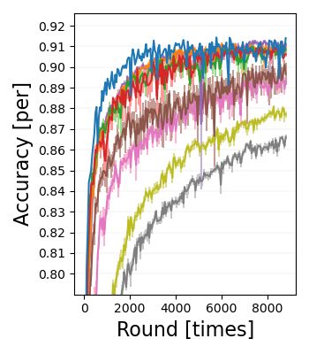
Asynchronous Decentralized Optimization with Implicit Stochastic Variance Reduction
                                                                           Node #2              Iteration time   round 1 (K=8)             round 2 (K=8)
Another important approach towards addressing the gradient                                       Node #1 U U X U U U U X U U U U U X U X U U U U
                                                                                      Node #3
drift issue is to solve a linearly constrained cost function     Node #1
                                                                                                 Node #2 U U X U U U U U U U U U U U U X U U U U
minimization problem to make the model variables iden-
                                                                                                 Node #3 U U U U X U U U U U U U U U U U U U X U
tical among the nodes. A basic solver for this problem
applies a primal-dual formalism using a Lagrangian func-
                                                                   Edge                          Node #N U U U U X U U X U U U U U X U U U U X U
tion. Representative algorithms on decentralized networks                   Node #4
                                                                                                         U Local node update     X Exchange between nodes
are the Primal-Dual Method of Multipliers (PDMM) (Zhang
                                                                   Figure 1. Decentralized network with asynchronous arbitrary node
& Heusdens, 2017; Sherson et al., 2018) and its extension
                                                                   connections and example procedure/communication schedule.
to non-convex DNN optimization named Edge-Consensus
Learning (ECL) (Niwa et al., 2020). When applying PDMM
to centralized networks, it reduces to the recently developed      ate and confirm the advantages of the proposed algorithms
FedSplit method (Pathak & Wainwright, 2020). By using              using benchmark image classification problems with both
the primal-dual formalism, the gradient modification terms         convex and non-convex cost functions (Sec. 7).
result naturally from the dual variables associated with the
model constraints. However, without a careful parameter            2. Preliminary steps
search to control the constraint strength, this approach may
not be effective in preventing gradient drift.                     We define symbols and notation in subsection 2.1. In sub-
                                                                   section 2.2, definitions that are needed for the convergence
SVR may be applicable even for the primal-dual formalism.          analysis are summarized.
In fact, it was recently reported in (Rajawat & Kumar, 2020)
that externally calculated control variates using, e.g., SVRG      2.1. Network settings and symbols
or SAGA can be added to the stochastic gradient of the             We now introduce the symbols and notations used through-
update procedure of PDMM. It is natural to assume that the         out the paper. Let us consider a decentralized network in
primal-dual formalism and SVR are not independent, but             Fig. 1, a set N of N local nodes is connected with arbi-
linked because both approaches are expected to be effective        trary graphical structure G(N , E), where E is a set of E
in terms of gradient drift reduction. Hence it is desirable to     bidirectional edges. A local node communicates with only
develop an algorithm that simultaneously takes advantage           a small number of fixed nodes in an asynchronous man-
of both approaches when computing the gradient control             ner. We denote set cardinality by | · |, so that N = |N |
variates instead of adding SVR externally to an existing           and E = |E|. The index set of neighbors connected to
method as (Rajawat & Kumar, 2020). Thus, we propose to             the i-th node is written as Ei = {j ∈ N |(i, j) ∈ E}. For
derive the control variates by solving a model constrained
minimization problem with a primal-dual formalism. Since                 P the number of edges, we use Ei = |Ei |, implying
                                                                   counting
                                                                   E = i∈N Ei . The data subsets xi are sets of cardinality
the constraint strength control parameter is included in a         |xi | containing ζ-dimensional samples available for each
primal-dual formalism, its optimal selection is natural. Thus,     local node i ∈ N . The xi may be heterogeneous, which
our novel approach represents an advance over many SVR             implies that xi and xj (i 6= j) are sampled from different
studies for decentralized optimization as it eliminates the        distributions. A communication schedule example is shown
implementational ambiguity of the control variates.                in Fig. 1. Assuming that the computational/communication
In this paper, we propose ECL-ISVR, which reformulates             performance of all local nodes is similar, K updates will be
the primal-dual formalism algorithm (ECL) such that it im-         performed at each local node for each node communication
plicitly includes the gradient control variates of SVR (see        round r ∈ {1,..., R}, namely each round contains K inner
Sec. 5). By inspection of the physical meaning of e.g., dual       iterations for each edge. Each node communicates once per
variables in ECL, we noticed that they are proportional to         round and the set of neighbor nodes connected with node i
the local gradient expectation, which are components of the        at iteration (r, k) is denoted by Eir,k .
gradient control variates of SVR. By optimally selecting           Our distributed optimization procedure can be applied to any
the constraint strength control parameter to scale dual vari-      ML model. Prior to starting the training procedure, identical
ables, the update procedure matches that of SVR. By doing          model architectures and local cost functions fi are defined
so, we avoid the implementational ambiguity of the control         for all nodes (fi = fj | i, j ∈ N ). The cost function at local
variates of SVR because they are implicitly updated in the         node i is fi (wi ) = Eχi ∼xi [fi (wi ; χi )], where wi ∈ Rm
primal-dual formalism algorithm. Since it eliminates addi-         represents the model variables at the i-th local node and
tional external operations as in (Rajawat & Kumar, 2020),          χi denotes a mini-batch data sample from xi . The cost
the proposed algorithm is expected to have small update            function fi : Rζ → R is assumed to be Lipschitz smooth
errors and to be robust in practical scenarios. We provide a       and it can be convex or non-convex (e.g., DNN). Thus, fi
convergence analysis for ECL-ISVR for the strongly convex,         is differentiable and the stochastic gradient is calculated as
general convex, and non-convex cases in Sec. 6. We evalu-          gi (wi ) = ∇fi (wi ; χi ), where ∇ denotes the differential op-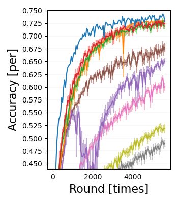
Asynchronous Decentralized Optimization with Implicit Stochastic Variance Reduction

erator. Our goal is to find the model variables that minimize        control variate ci , respectively, for correcting the gradient
the global cost function f (w) = N1 i∈N fi (wi ) while
                                        P
                                                                     on the i-th node as
making the local node models identical as much as possible                            ḡi (wi ) ← gi (wi ) + c̄i − ci ,           (3)
(wi = wj ), where the stacked model variables are given by
w = [w1T ,..., wN ] ∈ RN m and T denotes transpose.
                T T                                                  where the modified gradient is unbiased as the global variate
                                                                     is c̄i = Ej,r,k [gj (wi )] and the local control variate is ci =
2.2. Definitions                                                     Er,k [gi (wi )], where Ej,r,k and Er,k denote expectation w.r.t.
                                                                     both nodes connected with i-th node (j ∈Ni ) and time (r, k)
Next, we list several definitions that are used in the theoreti-
                                                                     and that w.r.t. time, respectively. It immediately follows
cal convergence analysis.
                                                                     that Ej,r,k [ḡi (wi )] = Er,k [gi (wi )]. The advantage of the
(D1) β-Lipschitz smooth: When fi is assumed to be Lips-              approach is that the variance of ḡi (wi ) is guaranteed to
chitz smooth, there exists a constant β ∈ [0, ∞] satisfying          be lower than that of gi (wi ) if Var[ci ] ≤ 2Cov[gi (wi ), ci ].
                                                                     GT-SVR (Xin et al., 2020) integrates SVR techniques into
  k∇fi (wi ) − ∇fi (ui )k ≤ βkwi − ui k,          (∀i, wi , ui ).
                                                                     DSGD for a fully-connected decentralized network.
This assumption implies the following inequality:                    It is discussed above that the gradient modification of (3)
 fi (ui ) ≤ fi (wi ) + h∇fi (wi ), ui − wi i +   β           2       results in gradient variance reduction. However, the imple-
                                                 2 kui − wi k .
                                                                     mentation of the control variates {c̄i , ci } is ambiguous. For
(D2) α-convex: When fi is assumed to be convex, there                a better implementation, the modification must be formu-
exists a constant α ∈ (0, β) satisfying for any two points           lated as the result of a change in the cost function. Based on
{wi , ui },                                                          such a cost function perspective, we provide mathematically
                                                                     rigorous derivations of distributed consensus algorithms that
 fi (ui ) ≥ fi (wi ) + h∇fi (wi ), ui − wi i + α2 kui − wi k2 .      facilitate further extension in the future.
Although α = 0 is allowed for general convex cases, α > 0            4. Primal-dual formalism
is guaranteed for strongly convex cases.
                                                                     4.1. Problem definition
(D3) σ 2 -bounded variance: gi (wi ) = ∇fi (wi ; χi ) is an
unbiased stochastic gradient of fi with bounded variance,            DSGD solves the decentralized model learning problem
                                                                     using a straightforward cost minimization approach (1). In-
        E[kgi (wi ) − ∇fi (wi )k2 ] ≤ σ 2     (∀i, wi ).             stead, we reformulate this problem as a more general linearly
                                                                     constrained minimization problem that is more effective in
3. Average consensus and its SVR application                         making the model variables identical across the nodes by
                                                                     reducing gradient drift:
Average consensus algorithms, such as DSGD, aim to solve
a simple cost minimization problem:                                    inf f (w) s.t. Ai|j wi + Aj|i wj = 0, (∀i∈N , j ∈Ei ), (4)
                                                                       w
                                                                     where Ai|j ∈Rm×m is the constraint parameter for the edge
                          inf w f (w).                         (1)
                                                                     (i, j) at node i. Since the set of Ai|j must force the model
The algorithms follow model averaging with a local node              variables to be identical over all nodes, we use identity
update based on stochastic gradient descent (SGD) using the          matrices with opposite signs, {Ai|j , Aj|i } = {I, −I}.
forward Euler method with step-size µ (>0) as wir,k+1 =              The linearly constrained minimization problem for convex
wir,k − µgi (wir,k ), where r labels the update round and k          cost function can be solved using a primal-dual formalism
denotes inner iteration. The forward update procedure is             (Fenchel, 1949). An effective approach to solve (4) on an
decomposed into K updates of wi performed on N local                 asynchronous decentralized network is PDMM (Zhang &
nodes. In e.g., FedProx (Li et al., 2019), a normalization           Heusdens, 2017; Sherson et al., 2018) and its extension
term to make the N node model variables be closer with               to optimize non-convex DNN models, ECL (Niwa et al.,
weight υ (>0) is added to the cost function as                       2020). Then, fi is assumed to be β-Lipschitz smooth but not
                                                                     necessarily convex, and it is natural to solve the majorization
       inf w f (w) + υ2 i∈N j∈Ei kwi − wj k2 .
                         P      P
                                                        (2)
                                                                     minimization of fi by defining a locally quadratic function
It has been reported that in heterogeneous data settings             qi around wir,k ,
and/or long communication intervals, (K 6= 1), so-called             qi (wi )=fi (wir,k )+ gi (wir,k ), wi − wir,k + 2µ
                                                                                                                      1
                                                                                                                        kwi − wir,k k2 .
gradient drift commonly occurs in average consensus algo-
rithms. An approach that aims to address this issue is to            When the step-size µ is sufficiently small, µ ≤ 1/β, then
apply an SVR method to DSGD, such as SVRG (Johnson &                 qi (wi ) ≥ fi (wi ) is guaranteed
                                                                                                   P everywhere. By replacing
Zhang, 2013) and SAGA (Defazio et al., 2014). A modified             f (w) in (4) by q(w) = N1 i∈N qi (wi ), a dual problem
gradient ḡi (wi ) is obtained by using global c̄i and local         can be defined.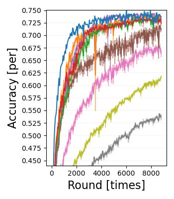
Asynchronous Decentralized Optimization with Implicit Stochastic Variance Reduction

To formulate the dual problem, we first define some vari-               Algorithm 1 Previous ECL (Niwa et al., 2020)
ables. Let A = Diag{[A1 ,..., AN ]} be a block diago-                    1: . Set wi = wj = ui|j (∼ Norm), zi|j = 0, fi , µ, ηi , ρi ,
nal matrix with the Ai = Diag{[Ai|Ei (1) ,..., Ai|Ei (Ei ) ]} ∈               xi , Ai|j
REi m×Ei m associated with the linear constraints. We                    2: for r ∈ {1, . . . , R} (Outer loop round) do
will use lifted dual variables for controlling the constraint            3:   for i ∈ N do
strength to facilitate asynchronous node communication.                  4:      for k ∈ {1, . . . , K} (Inner loop iteration) do
The lifted dual variables are written as λ=[λT1 , λT2 ,..., λTN ]T ,     5:         . Stochastic gradient calculation
with each lifted dual variable element held at a node relat-             6:         gi (wi ) ← ∇fi (wi , χi )
ing to one of its neighbours, λi =[λTi|Ei (1) ,..., λTi|Ei (Ei ) ]T ∈               . Update local primal and lifted
                                                                         7:
                                                                                                                  P dual variables
REi m . We will use an indicator function to enforce the                 8:         wi ← {wi − µgi (wi ) + µ j∈Ei (ηi ATi|j zi|j
equality of the lifted variables, λi|j = λj|i . For this pur-                          +ρi ui|j )}/(1 + µEi (ηi + ρi ))
pose, we define ιker(b) as the indicator function that takes             9:              for j ∈ Ei do
the value 0 for b = 0 and is ∞ elsewhere. Finally, let q ? be           10:                 yi|j ← zi|j − 2Ai|j wi
the convex conjugate of q. Then, the dual problem of (4)                11:              end for
can be formulated as (refer to (Niwa et al., 2020) for more             12:              . Procedure when communicated with j-th node
detail):                                                                13:              for j ∈ Eir,k (at random time) do
              inf λ q ? (JT AT λ) + ιker(I−P) (λ),                (5)   14:                 communicatej→i (wj , yj|i )
                                                                        15:                 ui|j ← (wj
where the mixing matrix J connects w and λ and is given
by J = Diag{[J1 ,..., JN ]} composed of Ji = [I,..., I]T ∈                                          yj|i              (PDMM-SGD)
                                                                        16:                zi|j ←   1        1
REi m×m and where P ∈ REm×Em denotes the permuta-                                                   2 zi|j + 2 yj|i   (ADMM-SGD)
tion matrix that exchanges the lifted dual variables between            17:        end for
connected nodes as λi|j        λj|i (∀i ∈ N , j ∈ Ei ). We              18:      end for
note that the convex conjugate
                                 function is q ? (JT AT λ) =           19:   end for
supw hλ, AJwi − q(w) . The indicator function that en-                  20: end for
forces equality on the lifted dual variables takes the value
zero only when (I − P)λ = 0 is satisfied.
                                                                        where the penalty term η2 kAJw − z r,k k2 (η > 0) in (6)
4.2. Update rules of ECL
                                                                        results from the linear constraints in (4). It reduces the gra-
We now briefly review the update rules of ECL, which aim                dient drift for each local node, so that the model variables
to solve (5). Since the two cost terms in (5) are ill-matched           over the N nodes are close. The update rules (6)–(8) can
because the indicator function is nondifferentiable, it is dif-         be decomposed into procedures on the local nodes, as sum-
ficult to reduce overall cost by, e.g., subtracting a scaled            marized in Alg. 1. A pair of a primal model variable and
cost gradient. In such situations, applying operator split-             a dual variable {wj , yj|i } or their update differences are
ting e.g., (Bauschke et al., 2011; Ryu & Boyd, 2016) can                transmitted between nodes according to the communication
be effective. The existing form of ECL allows two flavors               schedule of Fig. 1. Since DRS uses averaging with the
of operator splitting, Peaceman-Rachford Splitting (PRS)                previous value, the computation memory of ADMM-SGD
(Peaceman & Rachford, 1955) and Douglas-Rachford Split-                 (DRS) is larger than that of PDMM-SGD (PRS).
ting (DRS) (Douglas & Rachford, 1956), to obtain recursive              In PDMM and ECL, the following problems (P1), (P2)
variable update rules associated with PDMM (Zhang &                     remain unsolved:
Heusdens, 2017; Sherson et al., 2018) and ADMM (Gabay
                                                                        (P1) Non-optimal ηi : Since ηi is associated with constrained
& Mercier, 1976), respectively. In ECL, the augmented
                                                                        force strength, it is empirically scaled such that it is inversely
Lagrangian problem, which adds a model proximity term
ρ               r,k 2                                                   proportional to the parameters,
                                                                                                √           i.e., the number of model
2 kJw − PJw        k (ρ ≥ 0) to qi , is solved. The resulting
                                                                        element e as ηi ∝ 1/ e, similar to model initialization of
alternating update rules of the primal variable w and aux-
                                                                        (He et al., 2015). In our pre-testing using open source2 , ECL
iliary lifted dual variables {y, z} constitute PDMM-SGD
                                                                        requires careful selection of ηi to prevent gradient drift.
(PRS) and ADMM-SGD (DRS):
                                                                        (P2) Doubled communication requirement: In ECL, a pair
  wr,k+1 = arg min q(w)
                   w                                                    of primal and dual variables {wj , yj|i } are transmitted,
            η
                         z r,k k2 + ρ2 kJw − PJwr,k k2 , (6)            whereas DSGD exchanges only wj . When the variable up-

          + 2 kAJw −
      r,k+1    r,k                                                      date dynamics is stable, ignoring the proximity term (ρi =0)
  y        =z      − 2AJwr,k+1 ,                                 (7)
            (                                                           may be allowed. Then, ECL transmits only yj|i , where its
                Py r,k+1                 (PDMM-SGD)                     variable dimension is identical to that of wj .
  z r,k+1 =     1
                                                    ,            (8)
                2 Py
                     r,k+1
                           + 12 z r,k    (ADMM-SGD)                           2
                                                                                  https://github.com/nttcslab/edge-consensus-learning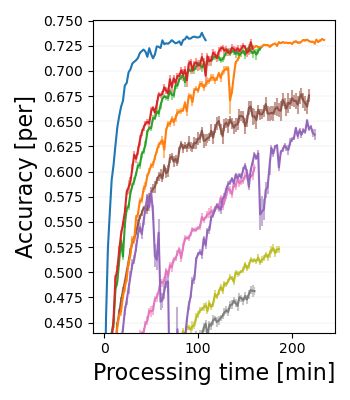
Asynchronous Decentralized Optimization with Implicit Stochastic Variance Reduction

5. Proposed algorithms (ECL-ISVR)                                                    P(r−1)/2
                                                                                =2      l=1     (Pu2l − u2l−1 )      (PRS).         (9)
As noted in Sec. 1, it is natural to assume that the primal-
dual formalism (ECL) and SVR must be related because                  In the next round (r + 1 is then even), the update is
both approaches aim to reduce gradient drift. More specif-                          P(r−1)/2
ically, the wi -update procedure in Alg. 1 is similar to the          AT z r+1,0 =2 l=1      (Pu2l+1−u2l )+2Pur (PRS). (10)
gradient modification of SVR in (3), as ηi ATi|j zi|j is added        Remembering that the ui|j represents the model variables,
to the stochastic gradient. If the gradient control variates of       (9) and (10) show that AT z in PRS is the cumulative sum
SVR can be represented by means of dual variables with op-            of model differences between nodes and it is updated every
timal ηi -selection in ECL, we can eliminate the ambiguities          two rounds.
in control variate implementation of SVR. Hence, the aim
of this section is to derive the SVR gradient modification            We now compare the results (9) and (10) to SVRG and
(3) by simply reformulating the update procedure in Alg. 1.           SAGA. There similar model differences between nodes with
                                                                      appropriate scaling are used to represent the global control
In Subsec. 5.1, we start with investigating the physical              variate c̄i = Ej,r,k [gj (wi )] (j ∈Ei ). To cancel out the effect
meaning of various terms (e.g., ATi|j zi|j ) and reformulate          of the step-size µ, the number of the inner loop   P iteration K,
the wi -update procedure to match that of SVR. This will              and that of connected nodes Ei , multiplying j∈Ei ATi|j zi|j
include optimal ηi -selection, thus solving (P1). After refor-        with −1/(µKEi ) is the optimal choice for PRS. Assuming
mulation, the wi -update procedure follows SVR, achieving             that r is an odd number, this results in
a stable variable update dynamics and additional model
                                                                           1
                                                                                  P        T    r,0
normalization will be unnecessary, (ρi = 0), thus halving              − µKE  i    j∈Ei Ai|j zi|j
the communication requirement and solving (P2). Our new                                  P(r−1)/2
                                                                            1
                                                                                                      2(u2l−1   − u2l
                                                                                  P
                                                                       = µKE        j∈Ei     l=1          i|j       j|i ) (PRS). (11)
algorithms, ECL-ISVR composed of PDMM-ISVR (PRS)                                i

and ADMM-ISVR (DRS), are summarized in Subsec. 5.2.                   Similarly to PRS, substituting (7) into the update rule of
5.1. The correspondence between ECL and SVR                           DRS (8) with initialization z 1,0 =0 results in
We first discuss some preliminaries needed for investigat-            AT z r+1,0 = 12 AT P(z r,0 − 2Aur ) + 12 AT z r,0
ing the terms in Alg. 1. The permutation matrix satisfies
                                                                      = 12 AT (I+P)z r,0 − 12 AT (PAPP+A)ur−1 −AT PAPPur
PP = I, furthermore AT A = I, and PAP = −A be-                                                 Pr−1
cause {Ai|j , Aj|i } = {I, −I}. The mixing matrix satifies            = 12 AT (I + P)z 1,0 + 21 l=1 (P − I)ul + Pur
JT J = Diag{[E1 I,..., EN I]}.                                             Pr−1
                                                                      = 21 l=1 (P − I)ul + Pur         (DRS),        (12)
To model the update lag of the variables resulting from asyn-
chronous communication (variables are exchanged once per              for any r. Although an offset Pur is added in (12), this can
K inner iterations with random timing for each edge as                be ignored as it is just a fraction that arises in the recursive
shown in Fig. 1) we define an additional variable to keep             formulation of model differences between nodes. It is ap-
track of the updates through the individual edges for the             propriate for DRS to selectP −1/(µKEi ) as scaling factor.
                       r,κ(i,j,r)                                     Then, multiplying with j∈Ei ATi|j zi|j results in
round as uri|j = wi                 ∈ Rm , where κ(i, j, r) denotes
the inner iteration index for communicating from the i-th                   1
                                                                                P          T    r+1,0
                                                                       − µKE  i   j∈Ei Ai|j zi|j
node to the j-th in round r. Since the dual variables are asso-             1
                                                                                P       Pr−1 1 l            l        r
ciated with the primal variables as in (7) and transmitted be-         = µKE  i   j∈Ei (     l=1 2 (ui|j − uj|i ) − uj|i ) (DRS). (13)
tween nodes by (8), it is natural to represent ATi|j zi|j ∈Rm         From (11) and (13), it is found that j∈Ei ATi|j zi|j with
                                                                                                                  P
considering the update lag by using uri|j . This variable
                                                                      appropriate scaling 1/(µKEi ) is associated with the global
can be stacked as u = [uT1 ,..., uTN ] ∈ REm composed of              control variates c̄i . However, difference between PRS and
ui =[uTi|Ei (1) ,..., uTi|Ei (Ei ) ]T ∈REi m .                        DRS exists, namely the primal model variables of the same
To investigate the physical meaning of ATi|j zi|j in Alg. 1,          round are used in DRS as (uli|j − ulj|i ), while those of a
we substitute the PRS update procedure (7) into (8) with              different round are used in PRS as (u2l−1          2l
                                                                                                               i|j − uj|i ). While
initialization z 1,0 = 0, with the replacement of Jw in (7)           the performance differences between PRS and DRS are
by u to model communication lags. The result is different             investigated in the experiments in Sec. 7, we expect the
when r is an odd number and when it is an even number.                convergence rate not to differ significantly since there are no
When r is an odd number, it results in                                essential differences in the physical meaning of the variables
                                                                      defined in (11) and those in (13).
AT z r,0 =AT P(z r−1,0 − 2Aur−1 )
                                                                      Since the existing terms in Alg. 1 are associated with the
         =AT P(z r−2,0 − 2Aur−2 ) − 2AT PAur−1
                       P(r−1)/2 T                                     global control variate, we would like to see if we can also
         =AT Pz 1,0 − 2 l=1    A (PAPPu2l +Au2l−1 )                   identify the local control variate ci = Er,k [gi (wi )] within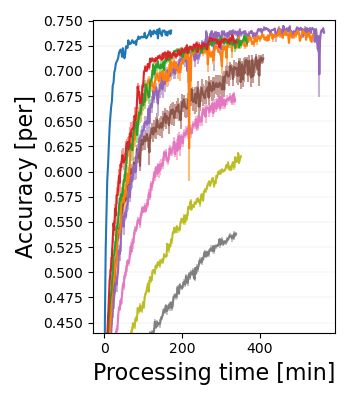
Asynchronous Decentralized Optimization with Implicit Stochastic Variance Reduction

ECL. To this purpose, let us reformulate the wi -update pro-          Algorithm 2 Proposed ECL-ISVR
cedure in Alg. 1 such that it matches with SVR’s update rule           1: . Set wi =wj (∼Norm), zi|j = 0, µ, xi , Ai|j
(3) with ρi = 0 to reduce the communication requirements:              2: for r ∈ {1, . . . , R} (Outer loop round) do
wir,k+1                                                                3:   for i ∈ N do
                                                                       4:      for k ∈ {1, . . . , K} (Inner loop iteration) do
=(wir,k −µgi (wir,k )+µηi           T    r,k
                            P
                               j∈EiAi|j zi|j )/(1+µηi Ei ) (14)        5:         . Stochastic gradient calculation
        µηi Ei
=(1− 1+µη        )(wir,k −µgi (wir,k ))+ 1+µη
                                           µηi     P       T    r,k    6:         gi (wi ) ← ∇fi (wi , χi )
            i Ei                              i Ei  j∈Ei Ai|j zi|j
                                                                       7:         . Update local primal and lifted dualP variables
= wir,k − µ[gi (wir,k ) + 1+µη
                            ηi                            r,k
                                    { j∈Ei(wir,k − ATi|j zi|j                     wi ← wi − µ[gi (wir,k ) + µKE  1
                                     P
                               i Ei
                                                              )        8:                                           i
                                                                                                                      {   j∈Ei

        − µEi gi (wir,k )}].                                (15)
                                                                                                          r,k
                                                                                          (wir,k − ATi|j zi|j ) − µEi gi (wir,k )}]
                                                                       9:         for j ∈ Ei do
Hereafter, we write Υi = 1/(1 + µηi Ei ) ∈ [0, 1] to simplify
                                                                      10:            yi|j ←zi|j − 2Ai|j wi
notation. SincePwi is recursively updated following (14),
                                                                      11:         end for
the term ηi Υi { j∈Ei(wi −ATi|j zi|j )−µEi gi (wi )} in (15)
                                                                      12:         . Procedure when communicated with j-th node
can be written as a summation of three terms T1 , T2 , and T3 ,
                                                                      13:         for j ∈ Eir,k (at random time) do
ηi Υi { j∈Ei(wir,k − ATi|j zi|j
                            r,k
                                ) − µEi gi (wir,k )=T1 +T2 +T3 ,
       P
                                                                      14:            communicate
                                                                                           (         j→i (yj|i )

where                                                                                         yj|i              (PDMM-ISVR)
                                                                      15:            zi|j ←   1        1
                                                                                              2 zi|j + 2 yj|i   (ADMM-ISVR)
         (r−1)K+k−1 1,0
 T1 =ηi Υi         wi ,                                (16)
                         r,k                     r,k−1                16:        end for
 T2 = −ηi Υi j∈Ei{ATi|j zi|j − µηi Ei Υi (ATi|j zi|j
            P
                                                       +              17:      end for
               r,k−2
     Υi ATi|j zi|j   +,...,+Υi
                                (r−1)K+k−1          1,0
                                             ATi|j zi|j )}, (17)      18:   end for
                                                                      19: end for
 T3 =−µηi Ei Υi {gi (wir,k )+Υi gi (wir,k−1 )+
                                (r−1)K+k
     Υ2i gi (wir,k−2 )+,..., +Υi        gi (wi1,0 )}.   (18)
When the number of update iterations is sufficient, T1 can
                                                               c̄r,k         1            T    r,k   1    T   r,k−1
                                                                                P
be ignored because T1 → 0. In T2 and T3 , the summation of       i = − µKEi         j∈Ei{Ai|j zi|j − K (Ai|j zi|j   +
geometric progression weight is included. Investigating the       1         r,k−2             1 (r−1)K+k−1 T        1,0
                                                             (1− K  )ATi|j zi|j   +,..,+(1− K   )            Ai|j zi|j  )},(24)
infinite sum of this geometric progression, it is guaranteed
to be one, independently of ηi -selection, as                  cr,k     1        r,k         1
                                                                 i = K {gi (wi ) + (1 − K )gi (wi
                                                                                                     r,k−1
                                                                                                           )+
                                         µηi Ei Υi
     µηi Ei Υi (1 + Υi +,...,+Υ∞
                               i )=       1−Υi       = 1.   (19) (1− K ) gi (wir,k−2 )+,..,+(1− K
                                                                     1 2                        1 (r−1)K+k
                                                                                                  )        gi (wi1,0 )}. (25)
This indicates that the weighted summation in (17) and (18)           We now have found the surprising fact that the gradient con-
is an implementation of the expectation computation over              trol variates of SVR are implicitly included in the primal-
both outer (r) and inner iterations (k) as                            dual formalism (ECL) by optimally selecting ηi as (22).
                               r,k
    T2 = −ηi Υi j∈Ei (ATi|j zi|j
                 P
                                   − Er,k [ATi|j zi|j ]), (20)        That is, SVR originates from the model-constrained mini-
                                                                      mization problem in (4).
    T3 = −Er,k [gi (wi )] = −ci ,                           (21)
                                                                      5.2. Update rules of ECL-ISVR
where the mean of T2 will be zero and the time constant in            The final algorithm forms for our ECL-ISVR are summa-
the expectation computation is larger when increasing ηi .            rized in Alg. 2, where wi -update procedure is obtained by
Since T3 corresponds to a local control variate as in (21),           substituting (22) into (15). Compared with ECL in Alg. 1,
ηi must be selected such that T2 is matched with the global           it is upgraded (i) to include the optimization of ηi , which
control variate. From (11) and (13), we can set the optimal           results in the wi -update procedure matching SVR and (ii)
ηi as ηi Υi =1/(µKEi ), and this results in                           to halve the communication requirement as only the lifted
                    ηi = 1/(µEi (K − 1)),                   (22)      dual variable are transmitted between connected nodes (this
                                                                      communication requirement is the same as DSGD).
where the number of inner loops is imposed to be K ≥ 2
                                                                      It remains an open question whether it is possible to recover
since ηi > 0. Then, (15) is reformulated such that it follows
                                                                      the data from yj|i since this variable reflects the statisti-
the SVR update rule (3):
                                                                      cal properties of the data. Since the lifted dual variable
     wir,k+1 = wir,k − µ{gi (wir,k ) + c̄r,k  r,k
                                         i − ci },          (23)      is basically an update difference of model variables as in
                                                                      (11) and (13), it will not be possible to estimate the data or
where the gradient control variates are given by substituting
                                                                      even the model variable without tracking of yj|i over a long,
(23) into (17) and (18) as
                                                                      continuous time, with the initial model value wi1,0 .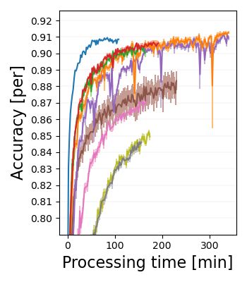
Asynchronous Decentralized Optimization with Implicit Stochastic Variance Reduction
                                                                                                                       Node #3
                                                                                (N1) Mul�plex ring      Node #2                       Node #4
  6. Convergence analysis of ECL-ISVR                                                       Node #1

  We conducted a convergence analysis for Alg. 2 for strongly
  convex, general convex, and non-convex cost functions. The                                                                                      Node #5
  detailed proofs are provided in the supplementary material.
                                                                                                      Node #8
                                                                                                                                      Node #6
  In our convergence analysis, we used the same mathematical                                                         Node #7
                                                                                                                                 Node #8
                                                                                                                                            Node #4
  techniques and proof strategies as the SCAFFOLD paper                         (N2) Random           Node #6
                                                                                                                  Node #1
  (Karimireddy et al., 2020).                                                               Node #3

  Proof sketch: We model the variable variance due to asyn-
  chronous communication lags in the supplementary material.
                                                                                                                                                 Node #7
  We combine these variances with the lemmas in the SCAF-                                               Node #5                  Node #2

  FOLD paper to complete our convergence analysis for Alg.
                                                                          Figure 2. Decentralized network composed of N =8 local nodes
  2. Note that difference between PDMM-ISVR and ADMM-
                                                                          with (N1) multiplex ring and (N2) random topologies
  ISVR is not considered because they just differs in model
                                                                          (T1) Fashion MNIST with a convex model: Fashion MNIST
  difference computation between connected nodes, as in (11)
                                                                          (Xiao et al., 2017) consists of 28 × 28 pixel of gray-scale
  and (13). The final results are given in the Theorem 1:
                                                                          images in 10 classes. The 60, 000 training samples are
  Theorem 1. Suppose that the functions {fi } satisfy (D1)                heterogeneously divided over N = 8 nodes. Each local node
  β-Lipschitz smooth and (D3) σ 2 -bounded variance. Then,                holds a different number of data and they are composed of
  in each of following cases with appropriate step-size setting,          8 randomly selected classes out of a total of 10 classes. The
  the output of ECL-ISVR (PDMM-ISVR and ADMM-ISVR)                        same 10, 000 test images are used on all nodes for evaluation.
  in Alg. 2 satisfies                                                     For the classification task, we use logistic regression with an
  Strongly convex: {fi } satisfies (D2) α-convex with α > 0,              affine transformation. The associated logistic loss function
                 1
  µ ∈ [0, min( 27βK    1
                    , 3αK )), R ≥ max( 27β    3
                                         2α , 2 ), then
                                                                          is convex.
          Emin                     α     1       σ2
                                                               (T2) Fashion MNIST with a non-convex model: The data
Ωcv ≤O             2
         Emin −1{αD0 exp(−min( 27βK   , 3K )R)+ αRK  (3+ 12
                                                          N )} , setting is the same as (T1). We applied a (non-convex)
  3
    where Ωcv = N1 i∈N E[(fi (wiR ) − fi (wi∗ ))], D02 =
                      P                                          ResNet-32 (He et al., 2016) with minor modifications. Since
   1
     P             1,0        ∗ 2            ∗        1,0 2      the statistics in mini-batch samples are biased in our hetero-
  N    i∈N (kfi (wi )−fi (wi )k + k∇fi (wi ) − E[ci ]k ),
  and Emin =min(Ei ) denotes the minimum number of edges         geneous data setting, group normalization (Wu & He, 2018)
  associated with a node and assumed to be Emin ≥2.              (1 group per 32 ch) is used instead of batch normalization
                                                                 (Ioffe & Szegedy, 2015) before each convolutional layer. As
  General convex: {fi } satisfies (D2) α-convex with α = 0,      a cost function, cross-entropy (CE) is used. wi is initialized
            1
  µ ∈ [0, 27βK ), R ≥ 1, then                                    by He’s method (He et al., 2015) with a common random
                                  q
                                             27βD02             seed.
        Ωcv ≤ O Emin { √σD0
                    Emin −1RKN
                                     3+ 12 +
                                      N       R     } .
                        1                                                 (T3) CIFAR-10 with a non-convex model: The CIFAR-10
  Non-convex: µ ∈ [0, 24βK ), R ≥ 1, then                                 data set consists of 32×32 color images in 10 object classes
                   √ q
         Ωnc ≤ O 23σ√ Q0      1+ 18
                                    +  3βQ0
                                            }  ,                          (Krizhevsky et al., 2009), where 50, 000 training images
                      RKN        N        R
                                      r,0
                                                                          are heterogeneously divided into N =8 nodes. Each local
  where Ωnc = N1 i∈N Ek∇fi (wi )k2 and
                     P
                                                              Q0    =     node holds 8 randomly selected data classes. For evaluation,
  1
    P           1,0        ∗
  N   i∈N (fi (wi ) − fi (w )).                                           the same 10, 000 test images are used for all nodes. CE
                                                                          with ResNet-32 using group normalization is used as a non-
  7. Numerical experiments                                                convex cost function.
  We evaluated the constructed algorithms by investigating                For all problem settings (T1)–(T3), squired L2 model nor-
  the learning curves for the case that statistically heteroge-           malization with weight 0.01 is added to the cost function.
  neous data subsets are placed at the local nodes. We aim to             The step-size µ = 0.002 and the mini-batch size 100 are
  identify algorithms that nearly reach the performance of the            used in all settings. Since the mini-batch samples are uni-
  reference case where all data are available on a single node.           formly selected from the unbalanced data subsets (8 out of
  7.1. Experimental setup                                                 10 classes), gradient drift will occur in all settings.
  Data set/models: We prepared the following three problem                Networks: To investigate the robustness in practical scenar-
  settings (T1)–(T3):                                                     ios (heterogeneous data, asynchronous/sparse communica-
                                                                          tion, and various network configurations), we prepared two
      3
        Further investigation is needed to provide a lower bound of       network settings composed of N =8 nodes, as in Fig. 2.
  Ωcv for finite R. In principle, the model variables {wiR } tend to be
  the same as the iteration R goes to ∞ due to the introduced control     (N1) Multiplex ring topology: Each node is connected with
  variants, which will eventually lead to nonnegativity of Ωcv .          its two neighboring nodes only (Ei =4, E =32).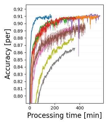
Asynchronous Decentralized Optimization with Implicit Stochastic Variance Reduction
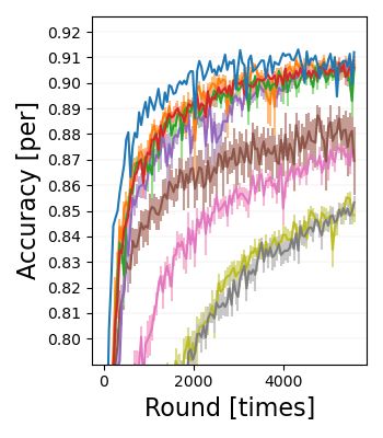
(T1)&(N1) (T1)&(N2) (T2)&(N1) (T2)&(N2) (T3)&(N1) (T3)&(N2)
Figure 3. Learning curves using test data set of (T1)-(T3) for (N1) multiplex ring and (N2) random topologies of Fig. 2. Node-averaged
classification accuracy is drawn as a solid line and one standard deviation is indicated by a light color.
(N2) Random topology: The number of edges for each In almost all settings, PDMM-ISVR (ECL-ISVR) per-
local node is non-homogeneous (Ei ∈ (2, 4), E = 20) and formed closest to the single-node reference scores and
identical over all experiments. second-best was ADMM-ISVR (ECL-ISVR). The perfor-
The communication between nodes was performed in an mance difference between them was slight. Their processing
asynchronous manner as shown in Fig. 1. The communica- time was almost the same as that of DSGD, but it is slower
tion for each edge is conducted once per K =8 local updates than the single-node reference due to the heterogeneous data
on average, with R=8, 800 rounds for (N1) and R=5, 600 division over the N nodes. Of the conventional algorithms,
rounds for (N2). the performance with PDMM-SGD (ECL) was better, but
its processing time was nearly 1.5 times that of DSGD.
Optimization algorithms: The proposed ECL-ISVR
This is caused by the doubled communication requirement
(PDMM-ISVR and ADMM-ISVR) in Alg. 2 is compared
issue. In addition, ADMM-SGD (ECL) was unstable in
with conventional algorithms, namely (1) DSGD, (2) Fed-
some cases, as shown in (T2)&(N2) and (T3)&(N2). This
Prox, (3) GT-SVR (implemented by GT-SAGA (Xin et al.,
may be caused by a non-optimal parameter choice {ηi , ρi }.
2020)), (4) D2 (Tang et al., 2018), and (5) ECL (PDMM-
√ GT-SVR takes the best score in (T1), however it did not
SGD and ADMM-SGD) in Alg. 1 with ηi = 3.0/ e, ρi =
reach the single-node reference scores in (T2) and (T3),
0.1. In addition, we prepared a reference model, which is a
even though the SVR technique was applied. This indicates
global optimization model trained by applying vanilla SGD
that our control variate implementation (24)-(25) provides
on a single node that has access to all data. The aim of all
robust performance in practical scenarios. FedProx, D2 , and
algorithms is to reach the score of the reference model.
DSGD did not work well, likely because of gradient drift.
Implementation: We constructed software that runs on a The proposed ECL-ISVR appears to be robust to network
server that has 8 GPUs (NVIDIA GeForce RTX 2080Ti) configurations as the network configuration does not affect
with 2 CPUs (Intel Xeon Gold 5222, 3.80 GHz). PyTorch performance significantly. In summary, the experiments
(v1.6.0) with CUDA (v10.2) and Gloo4 for node communi- confirm the effectiveness of the proposed ECL-ISVR.
cation was used. A part of our source code5 is available.
8. Conclusion
7.2. Experimental results
We succeeded in including the gradient control rules of SVR
Fig. 3 shows node-averaged classification accuracy learn- implicitly in the primal-dual formalism (ECL) by optimally
ing curves for the test data set/model (T1)–(T3) for both selecting ηi as (22). Through convergence analysis and
the multiplex ring (N1) and random (N2) topologies. The experiments using convex/non-convex models, it was con-
horizontal axis displays the number of rounds in the upper firmed that the proposed ECL-ISVR algorithms work well
row and the processing time in the lower row. While the in practical scenarios (heterogeneous data, asynchronous
processing time is the addition of (i) local node computation communication, arbitrary network configurations).
time for training/test data sets and (ii) communication time,
these are shown separately in the supplementary material. Acknowledgements
4 We thank Masahiko Hashimoto and Tomonori Tada for their
https://pytorch.org/docs/stable/distributed.html
5 help with the experiments.
https://github.com/nttcslab/ecl-isvr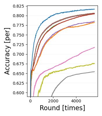
Asynchronous Decentralized Optimization with Implicit Stochastic Variance Reduction

References                                                       Jin, P. H., Yuan, Q., Iandola, F., and Keutzer, K. How
                                                                    to scale distributed deep learning?    arXiv preprint
Bauschke, H. H., Combettes, P. L., et al. Convex analysis
                                                                    arXiv:1611.04581, 2016.
  and monotone operator theory in Hilbert spaces, volume
  408. Springer, 2011.                                           Johnson, R. and Zhang, T. Accelerating stochastic gradient
                                                                   descent using predictive variance reduction. In Advances
Blot, M., Picard, D., Cord, M., and Thome, N. Gossip train-
                                                                   in Neural Information Processing Systems (NeurIPS), pp.
  ing for deep learning. arXiv preprint arXiv:1611.09726,
                                                                   315–323, 2013.
  2016.
                                                                 Kar, S. and Moura, J. M. Consensus+ innovations dis-
Chen, J. and Sayed, A. H. Diffusion adaptation strategies          tributed inference over networks: cooperation and sensing
  for distributed optimization and learning over networks.         in networked systems. IEEE Signal Processing Magazine,
  IEEE Transactions on Signal Processing, 60(8):4289–              30(3):99–109, 2013.
  4305, 2012.
                                                                 Karimireddy, S. P., Kale, S., Mohri, M., Reddi, S., Stich, S.,
Custers, B., Sears, A. M., Dechesne, F., Georgieva, I., Tani,      and Suresh, A. T. Scaffold: Stochastic controlled averag-
  T., and Van der Hof, S. EU personal data protection in           ing for federated learning. In International Conference
  policy and practice. Springer, 2019.                             on Machine Learning, pp. 5132–5143. PMLR, 2020.
Defazio, A., Bach, F., and Lacoste-Julien, S. SAGA: A            Krizhevsky, A., Hinton, G., et al. Learning multiple layers
  fast incremental gradient method with support for non-           of features from tiny images. 2009.
  strongly convex composite objectives. In Advances in
  Neural Information Processing Systems (NeurIPS), pp.           Li, T., Sahu, A. K., Zaheer, M., Sanjabi, M., Talwalkar, A.,
 1646–1654, 2014.                                                  and Smith, V. Federated optimization in heterogeneous
                                                                   networks. 1st Adaptive & Multitask Learning Workshop,
Douglas, J. and Rachford, H. H. On the numerical solu-             2019.
  tion of heat conduction problems in two and three space
 variables. Transactions of the American mathematical            Lian, X., Zhang, C., Zhang, H., Hsieh, C.-J., Zhang, W., and
 Society, 82(2):421–439, 1956.                                     Liu, J. Can decentralized algorithms outperform central-
                                                                   ized algorithms? A case study for decentralized parallel
Fenchel, W. On conjugate convex functions. Canadian                stochastic gradient descent. In Advances in Neural Infor-
  Journal of Mathematics, 1(1):73–77, 1949.                        mation Processing Systems (NeurIPS), pp. 5330–5340,
                                                                   2017.
Gabay, D. and Mercier, B. A dual algorithm for the solu-
  tion of nonlinear variational problems via finite element      Lim, W. Y. B., Luong, N. C., Hoang, D. T., Jiao, Y., Liang,
  approximation. Computers & mathematics with applica-             Y.-C., Yang, Q., Niyato, D., and Miao, C. Federated learn-
  tions, 2(1):17–40, 1976.                                         ing in mobile edge networks: a comprehensive survey.
                                                                   IEEE Communications Surveys & Tutorials, 2020.
He, K., Zhang, X., Ren, S., and Sun, J. Delving deep
  into rectifiers: Surpassing human-level performance on         Mao, Y., You, C., Zhang, J., Huang, K., and Letaief, K. B. A
  ImageNet classification. In Proceedings of the IEEE             survey on mobile edge computing: The communication
  International Conference on Computer Vision (ICCV), pp.         perspective. IEEE Communications Surveys & Tutorials,
 1026–1034, 2015.                                                 19(4):2322–2358, 2017.

He, K., Zhang, X., Ren, S., and Sun, J. Deep residual learn-     McMahan, B., Moore, E., Ramage, D., Hampson, S., and
  ing for image recognition. In Proceedings of the IEEE           y Arcas, B. A. Communication–efficient learning of deep
  Conference on Computer Vision and Pattern Recognition           networks from decentralized data. In Artificial Intelli-
  (CVPR), pp. 770–778, 2016.                                      gence and Statistics, pp. 1273–1282. PMLR, 2017.

Ioffe, S. and Szegedy, C. Batch normalization: Accelerating      Nesterov, Y. et al. Lectures on convex optimization, volume
   deep network training by reducing internal covariate shift.    137. Springer, 2018.
   arXiv preprint arXiv:1502.03167, 2015.
                                                                 Niwa, K., Harada, N., Zhang, G., and Kleijn, W. B. Edge-
Jiang, Z., Balu, A., Hegde, C., and Sarkar, S. Collaborative       consensus learning: Deep learning on p2p networks with
   deep learning in fixed topology networks. In Advances           nonhomogeneous data. In Proceedings of the 26th ACM
   in Neural Information Processing Systems (NeurIPS), pp.         SIGKDD International Conference on Knowledge Dis-
   5904–5914, 2017.                                                covery & Data Mining, pp. 668–678, 2020.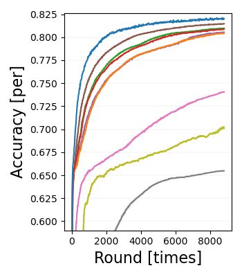
Asynchronous Decentralized Optimization with Implicit Stochastic Variance Reduction

Ormándi, R., Hegedüs, I., and Jelasity, M. Gossip learning   Xin, R., Khan, U. A., and Kar, S. Variance-reduced decen-
  with linear models on fully distributed data. Concurrency      tralized stochastic optimization with accelerated conver-
  and Computation: Practice and Experience, 25(4):556–           gence. IEEE Transactions on Signal Processing, 2020.
  571, 2013.
                                                               Zhang, G. and Heusdens, R. Distributed optimization using
Pathak, R. and Wainwright, M. J. Fedsplit: An algorith-          the primal-dual methomcd of multipliers. IEEE Trans-
  mic framework for fast federated optimization. 34th            actions on Signal and Information Processing over Net-
  Conference on Neural Inforamation Processing Systems           works, 4(1):173–187, 2017.
  (NeurIPS 2020), 2020.
                                                               Zhou, Z., Chen, X., Li, E., Zeng, L., Luo, K., and Zhang,
Peaceman, D. W. and Rachford, Jr, H. H. The numerical            J. Edge intelligence: Paving the last mile of artificial
  solution of parabolic and elliptic differential equations.     intelligence with edge computing. Proceedings of the
  Journal of the Society for industrial and Applied Mathe-       IEEE, 107(8):1738–1762, 2019.
  matics, 3(1):28–41, 1955.
Rajawat, K. and Kumar, C. A primal-dual framework for
  decentralized stochastic optimization. arXiv preprint
  arXiv:2012.04402, 2020.
Ram, S. S., Nedić, A., and Veeravalli, V. V. Distributed
  stochastic subgradient projection algorithms for convex
  optimization. Journal of optimization theory and appli-
  cations, 147(3):516–545, 2010.
Rockafellar, R. T. Convex analysis. Number 28. Princeton
  university press, 1970.
Ryu, E. K. and Boyd, S. Primer on monotone operator
  methods. Appl. Comput. Math, 15(1):3–43, 2016.
Sattler, F., Wiedemann, S., Müller, K.-R., and Samek, W.
  Robust and communication-efficient federated learning
  from non-iid data. IEEE Transactions on Neural Net-
  works and Learning Systems, 2019.
Sherson, T. W., Heusdens, R., and Kleijn, W. B. Derivation
  and analysis of the primal-dual method of multipliers
  based on monotone operator theory. IEEE Transactions
  on Signal and Information Processing over Networks, 5
  (2):334–347, 2018.
Shi, W., Cao, J., Zhang, Q., Li, Y., and Xu, L. Edge com-
  puting: Vision and challenges. IEEE Internet of Things
  Journal, 3(5):637–646, 2016.
Tang, H., Lian, X., Yan, M., Zhang, C., and Liu, J. D2 :
  decentralized training over decentralized data. arXiv
  preprint arXiv:1803.07068, 2018.
Wu, Y. and He, K. Group normalization. In Proceedings of
 the European Conference on Computer Vision (ECCV),
 pp. 3–19, 2018.
Xiao, H., Rasul, K., and Vollgraf, R. Fashion-mnist: a
  novel image dataset for benchmarking machine learning
  algorithms, 2017.
Xie, C., Koyejo, S., and Gupta, I. Asynchronous federated
  optimization. arXiv preprint arXiv:1903.03934, 2019.
You can also read