Fluctuations of finite-time Lyapunov exponents in an intermediate-complexity atmospheric model: a multivariate and large-deviation perspective ...
←
→
Page content transcription
If your browser does not render page correctly, please read the page content below
Nonlin. Processes Geophys., 26, 195–209, 2019
https://doi.org/10.5194/npg-26-195-2019
© Author(s) 2019. This work is distributed under
the Creative Commons Attribution 4.0 License.

Fluctuations of finite-time Lyapunov exponents in an
intermediate-complexity atmospheric model: a multivariate and
large-deviation perspective
Frank Kwasniok
Department of Mathematics, University of Exeter, Exeter, UK

Correspondence: Frank Kwasniok (f.kwasniok@exeter.ac.uk)

Received: 23 April 2018 – Discussion started: 2 May 2018
Revised: 7 July 2019 – Accepted: 8 July 2019 – Published: 31 July 2019

Abstract. The stability properties as characterized by              1   Introduction
the fluctuations of finite-time Lyapunov exponents around
their mean values are investigated in a three-level quasi-          The atmosphere is a high-dimensional non-linear chaotic dy-
geostrophic atmospheric model with realistic mean state and         namical system; its time evolution is characterized by sensi-
variability. Firstly, the covariance structure of the fluctuation   tivity to initial conditions (Lorenz, 1963; Kalnay, 2003). As a
field is examined. In order to identify dominant patterns of        consequence predictability is limited; small errors in the ini-
collective excitation, an empirical orthogonal function (EOF)       tial states progressively grow under the time evolution until
analysis of the fluctuation field of all of the finite-time Lya-    the forecast eventually becomes useless, that is, it is indistin-
punov exponents is performed. The three leading modes are           guishable from the invariant measure or climatology of the
patterns where the most unstable Lyapunov exponents fluc-           system. Understanding the structure of this inherent instabil-
tuate in phase. These modes are virtually independent of the        ity is key to improve forecasts at all timescales.
integration time of the finite-time Lyapunov exponents. Sec-           Sensitivity to initial conditions and perturbation growth in
ondly, large-deviation rate functions are estimated from time       non-linear dynamical systems are often quantified using Lya-
series of finite-time Lyapunov exponents based on the prob-         punov exponents (LEs; e.g. Eckmann and Ruelle, 1985; Ott,
ability density functions and using the Legendre transform          2002; Pikovsky and Politi, 2016). They describe the asymp-
method. Serial correlation in the time series is properly ac-       totic growth or decay of infinitesimal perturbations. A system
counted for. A large-deviation principle can be established         is chaotic if it has at least one positive Lyapunov exponent.
for all of the Lyapunov exponents. Convergence is rather            However, the predictability properties may vary substantially
slow for the most unstable exponent, becomes faster when            across state space. Finite-time (or local) Lyapunov exponents
going further down in the Lyapunov spectrum, is very fast for       (FTLEs) allow a characterization of the stability of a partic-
the near-neutral and weakly dissipative modes, and becomes          ular initial state with respect to a predefined prediction hori-
slow again for the strongly dissipative modes at the end of the     zon.
Lyapunov spectrum. The curvature of the rate functions at the          LEs have been calculated for various geophysical fluid
minimum is linked to the corresponding elements of the dif-         systems, ranging from highly truncated atmospheric mod-
fusion matrix. Also, the joint large-deviation rate function for    els (Legras and Ghil, 1985), to intermediate-complexity at-
the first and the second Lyapunov exponent is estimated.            mospheric models (Vannitsem and Nicolis, 1997; Schubert
                                                                    and Lucarini, 2015) and coupled atmosphere–ocean models
                                                                    (Vannitsem and Lucarini, 2016). A review has been pub-
                                                                    lished recently by Vannitsem (2017). Models tuned to real-
                                                                    istic conditions were found to possess quite a large number
                                                                    of positive LEs corresponding to a high-dimensional chaotic
                                                                    attractor.

Published by Copernicus Publications on behalf of the European Geosciences Union & the American Geophysical Union.
196                                                                 F. Kwasniok: Fluctuations of finite-time Lyapunov exponents

   The present paper investigates the fluctuations of FTLEs             where H is a scale height set to 8 km, and f0 is the Corio-
in an intermediate-complexity atmospheric model with real-              lis parameter at an average geographic latitude taken to be
istic mean state and variability. It focuses on two aspects that        45◦ N.
have found little attention in the context of geophysical fluid            The dissipative terms are given as follows:
systems thus far. Firstly, the covariance structure of the fluc-
                                                                        D1 = τN−1 R1,2
                                                                                   −2
                                                                                       (91 − 92 ) − kH ∇ 8 q̂1                          (5)
tuation field of the FTLEs is studied by means of a princi-
pal component (PC) or empirical orthogonal function (EOF)               D2 = − τN−1 R1,2
                                                                                     −2
                                                                                         (91 − 92 ) + τN−1 R2,3
                                                                                                            −2
                                                                                                                (92 − 93 )
analysis (Kuptsov and Politi, 2011). Secondly, we look at the
large-deviation behaviour of the FTLEs (Kuptsov and Politi,                    − kH ∇ 8 q̂2                                             (6)
2011; Laffargue et al., 2013; Johnson and Meneveau, 2015).              D3 = −τN−1 R2,3
                                                                                    −2
                                                                                        (92 − 93 ) − τE−1 ∇ 2 93 − kH ∇ 8 q̂3 .         (7)
A large-deviation principle links the FTLEs at long integra-
                                                                        They are Newtonian temperature relaxation with a radiative
tion times to the global LEs by providing a universal law for
                                                                        timescale of τN = 25 d, Ekman damping on the lowest level
the probability density of fluctuations of the FTLEs around
                                                                        with a spin-down timescale of τE = 1.5 d, and a strongly
the mean value. It can be expected to hold for Axiom A dy-
                                                                        scale-selective horizontal diffusion of vorticity and temper-
namical systems and, invoking the chaotic hypothesis, also
                                                                        ature. The q̂i is the time-dependent part of the potential vor-
for certain types of non-Axiom A systems. In particular, a
                                                                        ticity at level i, that is to say q̂i = qi −f −δi3 f0 h. The coeffi-
large-deviation law allows one to determine the probability
                                                                        cient of horizontal diffusion kH = τH−1 [nm (nm +1)]−4 is such
of very stable or very unstable atmospheric states.
                                                                        that harmonics of total wave-number nm = 21 are damped at
   The paper is organized as follows: in Sect. 2 the atmo-
                                                                        a timescale of τH = 1.5 d. The terms Si = Si (λ, µ) are dia-
spheric model is described; the methodology, which consists
                                                                        batic sources of potential vorticity which are independent of
of calculating LEs, the multivariate fluctuation analysis and
                                                                        time but spatially varying.
the large-deviation theory, is outlined in Sects. 3, 4 and 5;
                                                                           The model is considered on the Northern Hemisphere. The
the results are presented and discussed in Sect. 6; and some
                                                                        boundary condition of no meridional flow, vi (λ, 0) = 0, that
conclusions are drawn in Sect. 7.
                                                                        is to say vanishing stream function, 9i (λ, 0) = 0, is applied
                                                                        at the Equator on all three model levels. The horizontal dis-
2   The atmospheric model                                               cretization is spectral, triangularly truncated at total wave-
                                                                        number nm = 21. The number of degrees of freedom is 231
A quasi-geostrophic (QG) three-level model on the sphere,               for each level and N = 693 in total. The model is integrated
formulated in pressure coordinates, is used here as dynami-             in time using the third-order Adams–Bashforth scheme with
cal framework. The model is identical to that introduced by             a constant step size of 1 h.
Kwasniok (2007) except for the horizontal resolution and the               The variables of the QG model are listed in Table 1; the
coefficient of hyperviscosity. A very similar model was intro-          model parameters are listed in Table 2 with their dimensional
duced by Marshall and Molteni (1993). The dynamical equa-               and non-dimensional values.
tions are as follows:                                                      In order to get a model behaviour close to that of the
∂qi                                                                     real atmosphere, the forcing terms Si are determined from
     + J (9i , qi ) = Di + Si , i = 1, 2, 3,                  (1)       the European Centre for Medium-Range Weather Forecasts
 ∂t
where 9i and qi are the stream function and the potential               (ECMWF) reanalysis data by requiring that when comput-
vorticity at level i, respectively, and J denotes the Jacobian          ing potential vorticity tendencies for a large number of ob-
operator on the sphere. All variables are non-dimensional us-           served atmospheric fields, the average of these tendencies
ing the radius of the Earth as the unit of length and the inverse       must be zero (Roads, 1987); this is done in order for the en-
of the angular velocity of the Earth as the unit of time. The           semble of reanalysis data states to be representative of a sta-
three pressure levels are located at 250, 500 and 750 hPa. Po-          tistically stable long-term behaviour of the QG model. The
tential vorticity and the stream function are related by                timescale of horizontal diffusion τH is determined such that
                                                                        the slope of the kinetic energy spectrum at the truncation
               −2
q1 = ∇ 2 91 − R1,2 (91 − 92 ) + f                            (2)        level in the model matches that in the reanalysis data. See
       2       −2                 −2                                    Kwasniok (2007) for details on the parameter tuning proce-
q2 = ∇ 92 + R1,2   (91 − 92 ) − R2,3 (92 − 93 ) + f          (3)
                                                                        dure. The QG model exhibits a remarkably realistic mean
               −2
q3 = ∇ 2 93 + R2,3 (92 − 93 ) + f + f0 h,                    (4)        state and variability pattern of stream function and potential
                                                                        vorticity in a long-term integration (see Table 3).
where ∇ is the horizontal gradient operator, and f is
the Coriolis parameter. The Rossby deformation radii R1,2
and R2,3 have dimensional values of 575 and 375 km,                     3   Lyapunov exponents
respectively. The function h = h(λ, µ) represents a non-
dimensional topography which is related to the actual dimen-            We consider a non-linear autonomous dynamical system
sional topography of the Earth h∗ = h∗ (λ, µ) by h = h∗ /H ,            with state vector x = (x1 , . . ., xN )T governed by the evolu-

Nonlin. Processes Geophys., 26, 195–209, 2019                                     www.nonlin-processes-geophys.net/26/195/2019/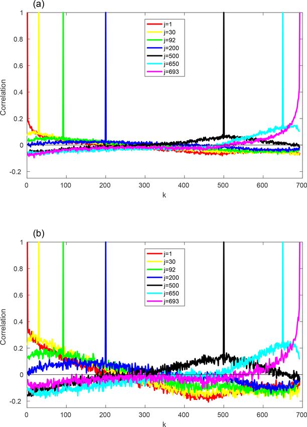
F. Kwasniok: Fluctuations of finite-time Lyapunov exponents                                                                               197

Table 1. Variables and fields in the QG model and their non-dimensionalization with the Earth’s radius a = 6.371 × 10⁶ m and the angular
velocity of the Earth  = 7.292 × 10⁻⁵ s−1 .

         Symbol                            Description                                               Unit        Non-dimensionalization
         t                                 Time                                                      s           −1
         λ (0 ≤ λ < 2π)                    Longitude (eastward)
         φ (0 ≤ φ ≤ π/2)                   Latitude
         µ = sin φ (0 ≤ µ ≤ 1)             Sine of latitude
         9i                                Stream function at level i                                m2 s−1      a2
         qi                                Potential vorticity at level i                            s−1
         q̂i                               Time-dependent part of potential vorticity at level i     s−1
         f = 2µ                            Coriolis parameter                                        s−1
         h                                 Topography of the Earth                                   m           H
         Si     p                          Diabatic forcing at level i                               s−2         2
         ui = − p1 − µ2 (∂9i /∂µ)          Zonal velocity (eastward)                                 m s−1       a
         vi = (1/ 1 − µ2 ) (∂9i /∂λ)       Meridional velocity (northward)                           m s−1       a

Table 2. Parameters in the QG model.

             Symbol     Description                                                 Dimensional value         Non-dimensional value
             R1,2       Rossby deformation radius between levels 1 and 2            575 km                    9.025 × 10⁻²
             R2,3       Rossby deformation radius between levels 2 and 3            375 km                    5.886 × 10⁻²
             τN         Timescale of temperature relaxation                         25 d                      50π
             τE         Timescale of Ekman damping                                  1.5 d                     3π
             τH         Timescale of horizontal diffusion at wave-number 21         1.5 d                     3π
                                                                                                              √
             f0         Coriolis parameter at 45◦ N                                 1.031 × 10⁻⁴ s−1            2
             H          Scale height                                                8 km

Table 3. Pattern correlation of various fields in the QG model with        where M is the resolvent matrix. If the system is ergodic,
the corresponding fields in ECMWF reanalysis data.                         then according to the theorem by Oseledets (1968) the limit
                                                                                                    1
                                                                           S = lim MT M
                                   q           q                                                2(t−t
                                                                                                         0)                               (11)
              Level      h9i i      h9i0 2 i       hq̂i0 2 i                    t→∞

              250 hPa     0.99         0.99         0.97                   exists and is the same for almost all initial conditions x 0 . The
              500 hPa     0.99         0.99         0.98                   (global) LEs are defined as
              750 hPa     0.96         0.97         0.94
                                                                           λj = log ωj , j = 1, . . ., N,                                 (12)
                                                                           where   {ωj }N
                                                                                        j =1are the positive eigenvalues of the matrix S.
tion equations                                                             The set of all LEs, usually presented in non-increasing order,
                                                                           is called the “Lyapunov spectrum”. The LEs are independent
dx                                                                         of the norm.
   = f (x).                                                       (8)         In order to characterize perturbation growth or decay over
dt                                                                                                                      (τ )
                                                                           a finite integration time τ the FTLEs 3j (x 0 ) are intro-
The linearized dynamics of a small perturbation δx are given               duced. There are three different definitions of FTLEs. One
as                                                                         can compute them by making reference to the backward, for-
                                                                           ward or covariant Lyapunov vectors – see e.g. Kuptsov and
d       ∂f                                                                 Parlitz (2012) for a review. In the limit of large integration
   δx =    δx.                                                    (9)
dt      ∂x                                                                 time τ , which is the main focus of the present study, all of the
                                                                           three definitions become more and more equivalent (Kuptsov
The propagation of the perturbation between time t0 with ini-              and Politi, 2011; Pazó et al., 2013). Here, we refer to the
tial state x 0 = x(t0 ) and time t (t > t0 ) can be written as             backward FTLEs as they are easiest to compute. They are
                                                                           calculated using the standard algorithm based on the Gram–
δx(t) = M(x 0 , t − t0 )δx(t0 ),                                 (10)      Schmidt orthogonalization (Shimada and Nagashima, 1979;

www.nonlin-processes-geophys.net/26/195/2019/                                           Nonlin. Processes Geophys., 26, 195–209, 2019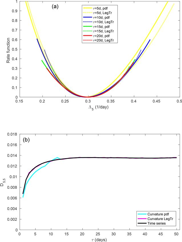
198                                                                 F. Kwasniok: Fluctuations of finite-time Lyapunov exponents

Benettin et al., 1980). An ensemble of N linearly indepen-              matrix D(τ ) defined as
dent perturbations is initialized and integrated forward in                                      T
                                                                         (τ )        (τ )       (τ )
time along with the non-linear model trajectory. A transient            D = 3 −λ 3 −λ                     τ
period is discarded for the trajectory to settle on the attrac-
tor of the system and for the perturbations to converge to                              τ L−1
                                                                                          X                       T
the backward Lyapunov vectors. Then, after every integration                        =         3(τ )
                                                                                                    − λ    3 (τ )
                                                                                                                  − λ   .            (17)
                                                                                        L α=0 α              α
time interval 1τ the perturbations are re-orthonormalized us-
ing a QR-decomposition performed via the Gram–Schmidt                   In the limit of large integration time τ we expect convergence
procedure. The FTLEs are obtained as                                    to the diffusion matrix D (Kuptsov and Politi, 2011; Pikovsky
                                                                        and Politi, 2016):
    (1τ )            (1τ )     1
3j          (x α ) = 3j,α =      log Rjj (tα , tα+1 ),
                              1τ                                        D = lim D(τ ) .                                              (18)
                                                                                    τ →∞
      α = 0, . . ., L − 1,                                  (13)
                                                                        The eigenvalues and eigenvectors of the symmetric, positive
where Rjj (tα , tα+1 ) are the diagonal elements of the upper           definite matrix D(τ ) are calculated:
triangular matrix R in the QR-decomposition resulting from                          (τ )        (τ ) (τ )
the integration between times tα and tα+1 . We have tα = t0 +           D(τ ) ej = νj ej .                                           (19)
                                      (τ )
α1τ and x α = x(tα ). The FTLEs 3j for larger integration
                                                                                                               (τ )
times τ = n1τ are obtained by averaging over n consecutive              The eigenvalues {νj }N j =1 are arranged in non-increasing or-
             (1τ )                                                      der. The eigenvectors form an orthonormal system:
values of 3j :
                                                                                                N
            n−1                                                          (τ )        (τ )
                                                                                                X            (τ ) (τ )
 (τ )     1X      (1τ )                                                 ej · ek =                       ej,i ek,i = δj k .           (20)
3j,α    =       3       , α = 0, . . ., L − 1.              (14)
          n i=0 j,α+i                                                                           i=1

                                                                        The fluctuation field of the FTLEs is expanded as
For all integration times τ , we keep time series of FTLEs of
                       (τ )
the same length L, {3j,α }L−1
                            α=0 , characterizing the stability of                              N
                                                                                                         (τ ) (τ )
                                                                                               X
the states     {x α }L−1
                     over the time horizon τ .                          3(τ )
                                                                         α −λ =                        yj,α ej                       (21)
                     α=0
                                                                                               j =1
   The FTLEs depend on the scalar product chosen in the
Gram–Schmidt orthogonalization procedure. Here, we use                                  (τ )          (τ )
                                                                        with yj,α = ej · (3(τ )
                                                                                           α − λ). The principal components
the total energy scalar product with its associated total energy             (τ )
norm (Ehrendorfer, 2000; Kwasniok, 2007). The dependence                {yj }Nj =1 are uncorrelated and their variance is given by the
of the FTLEs on the norm becomes increasingly weaker in                 corresponding eigenvalue:
the limit of large integration time τ .                                 D           E 1 L−1
   The FTLEs are related to the global LEs by                             (τ ) (τ )
                                                                                        X (τ ) (τ ) (τ )
                                                                         yj yk =            y y = ν j δj k .                         (22)
                                                                                      L α=0 j,α k,α
      (τ )
 lim 3 (x 0 ) = λj                                          (15)
τ →∞ j
                                                                        The steepness or complexity of the eigenvalue spectrum is
for almost all initial states x 0 and                                   characterized by the fraction of variance explained by the
                                                                                              (τ )
D       E                                                               principal component yj given as
   (τ )
 3j = λj                                                    (16)
                                                                                               (τ )
                                                                         (τ )
                                                                                   νj
for all τ , where h·i denotes an ensemble average over the              rj      = PN             (τ )
                                                                                                                                     (23)
attractor of the system which for ergodic systems can be es-                                k=1 νk
timated as a mean over a long time series.                              and the cumulative fraction of variance given as
                                                                               Pj      (τ )
                                                                         (τ )         νk
4     Multivariate fluctuation analysis                                 cj = Pk=1 N    (τ )
                                                                                            .                                        (24)
                                                                                  k=1 νk
The vector of global Lyapunov exponents is defined as
                                                                           As a possible further step, one may try to link the covari-
λ = (λ1 , . . ., λN )T and the fluctuation field as 3(τ ) − λ =

   (τ )               (τ )
                             T                                         ance structure of the FTLEs with investigations of the angles
  31 − λ1 , . . ., 3N − λN . We study the correlations be-              between the covariant Lyapunov vectors and the degree of
tween the fluctuations of the FTLEs; to do this, preferred              entanglement and interaction of the various unstable and sta-
patterns of collective excitation are extracted. A canonical            ble directions in tangent space (Yang et al., 2009). This is
approach is a principal component (PC) or empirical orthog-             related to the hyperbolicity and the inertial manifold of the
onal function (EOF) analysis based on the scaled covariance             system.

Nonlin. Processes Geophys., 26, 195–209, 2019                                               www.nonlin-processes-geophys.net/26/195/2019/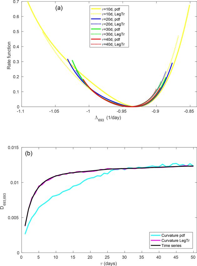
F. Kwasniok: Fluctuations of finite-time Lyapunov exponents                                                                   199

5        Large-deviation theory for FTLEs                         with the SCGF

Large-deviation theory (Kifer, 1990; Touchette, 2009) is a                        1          (τ )
                                                                  γj (θ ) = lim     log eτ θ3j .                              (32)
powerful approach from statistical physics for estimating the                τ →∞ τ
probability of rare events with many applications. It has re-
cently been applied to the behaviour of FTLEs at long in-         Introducing θ 0 = τ θ and then dropping the prime again we
tegration times (Kuptsov and Politi, 2011; Laffargue et al.,      get
2013; Johnson and Meneveau, 2015). In the following, large-
                                                                               1                    (τ )
                                                                                                  θ3j
deviation theory is briefly described in the form in which it     Ij (z) = lim sup θ z − log e              .            (33)
                                                                          τ →∞ τ θ∈R
is used in the present study.

5.1       Univariate theory                                       We expect convergence of the rate function Ij (z) as soon as
                                                                  the integration time τ is large enough for consecutive values
                                                                        (τ )
For a sequence of n identically distributed but not necessarily   of 3j taken over non-overlapping integration time inter-
independent random variables, {Xi }ni=1 , the sample mean                  (τ )          (τ )
                                                                  vals, 3j,α and 3j,α+n , to be independent. This is actually
              n
                                                                  an application of the block averaging method (Rohwer et al.,
           1X                                                     2015). Note, however, that convergence of the rate function
An =             Xi                                       (25)
           n i=1                                                  at a particular value of τ here does not guarantee that the
                                                                  probability density function is already in the large-deviation
is an unbiased estimator of and converges to the true mean,       limit at that value of τ .
hXi, as n → ∞. According to the Gärtner–Ellis theorem                The rate function Ij (z) has a unique zero and minimum at
(Touchette, 2009), if the scaled cumulant generating function     z∗ = λj , that is to say Ij (λj ) = 0 and Ij0 (λj ) = 0. The cur-
(SCGF)                                                            vature of the rate function at the minimum is linked to the
                                                                  diffusion matrix D as
                1    D      E
γ (θ ) = lim      log enθAn                               (26)
            n→∞ n                                                                        1            −1
                                                                  Ij00 (λj ) =              2  = Dj,j .                   (34)
exists and is differentiable everywhere, then An follows a                              (τ )
                                                                                  lim 3j − λj     τ
                                                                                  τ →∞
large-deviation principle,

p(An = z) ∼ exp[−nI (z)],                                 (27)    A second-order Taylor expansion of the rate function in the
                                                                  vicinity of λj ,
where the large-deviation rate function I (z) is independent of
                                                                          1
n and given as the Legendre–Fenchel transform of the SCGF:        Ij (z) ≈ Ij00 (λj )(z − λj )2 ,                             (35)
                                                                          2
I (z) = sup [θ z − γ (θ )].                               (28)
            θ∈R                                                   corresponds to a Gaussian probability density with mean λj
                                                                  and variance Dj,j /τ , recovering the central limit theorem
   The rate function I (z) is non-negative and strictly convex.   (CLT) as a limit case of large-deviation theory.
It has a unique zero and minimum at z∗ = hXi, that is to say
I (hXi) = 0 and I 0 (hXi) = 0. The curvature of the rate func-    5.2     Estimating the rate function
tion at the minimum is given as (Touchette, 2009)
                                                                  There are two ways of estimating the rate functions Ij (z)
    00                      1                                     from data: via the probability density function (cf., Eq. 30)
I (hXi) =                                  .              (29)
                   lim nh(An − hAn i)2 i                          or via the Legendre transform (cf., Eq. 33).
                  n→∞

   In view of Eq. (14), FTLEs immediately lend themselves         5.2.1    Probability density function approach
to large-deviation theory. For large integration time τ , one
would expect the probability density of the FTLE 3j to
                                                       (τ )       By inverting Eq. (30) we have
follow a large-deviation principle,                                                    1
                                                                                                (τ )
                                                                  Ij (z) = − lim         log p 3j = z .                       (36)
                                                                                  τ →∞ τ

      (τ )
p 3j = z ∼ exp[−τ Ij (z)],                               (30)
                                                                  We take a maximum likelihood approach for estimating the
                                                                                                             (τ )
where the large-deviation rate function Ij (z) is independent     rate function. The probability density of 3j is modelled as
of τ and given as

                                                                     (τ )
                                                                            1       h
                                                                                        (τ )
                                                                                             i
Ij (z) = sup [θ z − γj (θ )]                              (31)    p 3j = z = (τ ) exp −Uj (z)                                 (37)
            θ ∈R                                                            Zj

www.nonlin-processes-geophys.net/26/195/2019/                                     Nonlin. Processes Geophys., 26, 195–209, 2019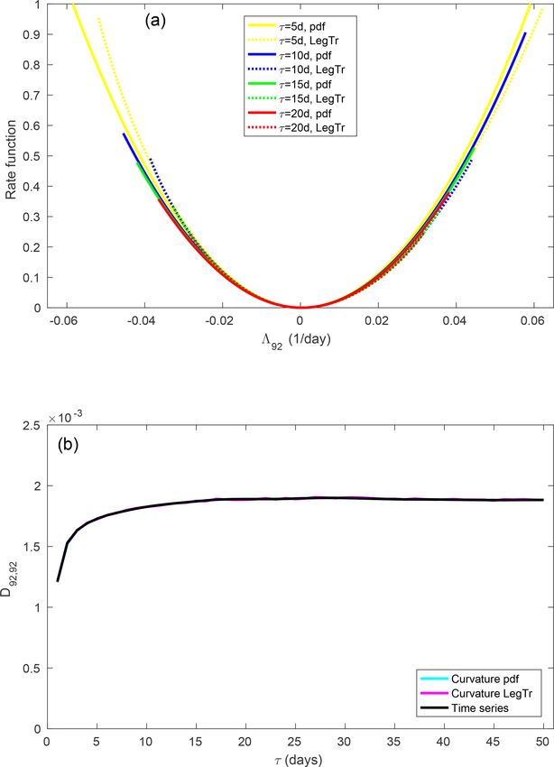
200                                                                                          F. Kwasniok: Fluctuations of finite-time Lyapunov exponents

with normalization constant                                                                      For each z, this is a convex optimization problem with a
                                                                                                 unique solution, if a solution exists. Rate functions obtained
                   Z∞
 (τ )
                             h
                                (τ )
                                     i                                                           via the Legendre transform method are guaranteed to be
Zj         =              exp −Uj (z) dz.                                             (38)       strictly convex with a unique zero and minimum at z∗ = λj .
                  −∞                                                                                Rate function estimates from the Legendre transform
                                                                                                 method converge as soon as τ = n1τ is large enough for suc-
                                          (τ )                                                                       (τ )
The potential function Uj (z) is expanded into a polynomial                                      cessive values of 3j over non-overlapping integration time
basis in standardized variables:                                                                             (τ )        (τ )
                                                                                                 intervals, 3j,α and 3j,α+n , to be independent. However, this
             M
                              !i                                                                 gives no indication of whether or not the probability den-
  (τ )           (τ ) z − λj
            X
Uj (z) =        βi               .                     (39)                                      sity function is actually already in the large-deviation limit.
                         (τ )
            i=1        σj                                                                        Therefore, here we consider both rate function estimates side
                                                                                                 by side.
                  (τ )                                                     (τ )
Here σj                  is the standard deviation of the FTLE 3j :
                                                                                                 5.3   Estimating the diffusion coefficients
                                                 "                        #1/2
                          2 1/2                  1 L−1
                                                       X  (τ )      2                          The diffusion coefficients Dj,j can be obtained from both
    (τ )             (τ )
σj         =        3j − λj         =                      3j,α − λj              .   (40)       rate function estimates as the inverse of the curvature at
                                                     L α=0
                                                                                                 the minimum (cf., Eq. 34). They can also be estimated
The parameter M determines the complexity of the model. In                                       directly from the time series of the FTLEs according to
order to have a normalizable probability density, we need M                                      Eq. (17). It can be shown that the estimates from the Leg-
                  (τ )                                 (τ )
to be even and βM > 0. The expansion coefficients {βi }M    i=1
                                                                                                 endre transform-based rate function and from the time se-
are determined by maximizing the likelihood function of the                                      ries are always the same; any differences just stem from the
        (τ )
data {3j,α }L−1
             α=0 . This is a convex optimization problem with
                                                                                                 error of the finite-difference approximation of the curvature
a unique maximum which is numerically stable to solve.                                           as the Legendre transform is not available in closed form.
Model selection is performed with the Bayesian information                                       For a Gaussian probability density model, that is M = 2 in
criterion.                                                                                       Eq. (39), the diffusion coefficient estimates from the proba-
   The estimate of the rate function is given as                                                 bility density-based rate function and from the time series are
                                                                                                 exactly the same; otherwise they are different.
                           1 h (τ )     (τ )
                                               i
Ij (z) = lim                  Uj (z) − Uj (z∗ ) ,                                     (41)       5.4   Multivariate theory
                      τ →∞ τ

where z∗ denotes the position of the minimum of the poten-                                       The large-deviation analysis can be extended to a multivari-
                (τ )
tial function Uj (z). Note that, for finite τ , we do not nec-                                   ate approach (Kuptsov and Politi, 2011; Johnson and Mene-
                ∗
essarily have z = λj as the mode of the probability density                                      veau, 2015). Let 3(τ ) now denote the column vector of any
      (τ )                                                                                       K-dimensional subset of the N FTLEs and λ the correspond-
of 3j may be different from its mean if the distribution is
skewed; however, we always have z∗ → λj as τ → ∞. One                                            ing vector of global LEs. We have 1 ≤ K ≤ N , where K = N
would now estimate Ij (z) from the probability density func-                                     corresponds to the full system and K = 1 recovers the uni-
           (τ )                                                                                  variate analysis. For large integration time τ , the joint prob-
tion of 3j for various large values of τ and look for con-
                                                                                                 ability density function of the K FTLEs would then follow a
vergence.
                                                                                                 large-deviation principle,
   The maximum likelihood method tends to provide very
smooth and convex rate functions although convexity is not                                       p 3(τ ) = z ∼ exp[−τ I (z)],                                (43)
strictly guaranteed. It clearly improves on earlier work (e.g.
Johnson and Meneveau, 2015) using histogram or kernel                                            where the joint large-deviation rate function I (z) is indepen-
density estimates for the probability density and treating the                                   dent of τ and given as the multivariate Legendre–Fenchel
normalization constant only in the Gaussian approximation.                                       transform
                                                                                                              1       h          D T (τ ) Ei
5.2.2             Legendre transform approach                                                    I (z) = lim sup θ T z − log eθ 3            .              (44)
                                                                                                         τ →∞ τ
                                                                                                                θ ∈RK

Alternatively, the rate functions Ij (z) can be determined                                          The joint rate function I (z) is non-negative and strictly
by numerically implementing the Legendre transform of                                            convex. It has a unique zero and minimum at z∗ = λ, that is
Eq. (33) (Rohwer et al., 2015) with the moment generating                                        to say I (λ) = 0 and ∂I /∂zj = 0 at z = λ. The Hessian ma-
function estimated by the sample mean over the time series:                                      trix of the joint rate function at the minimum is linked to the
                                                                                                 diffusion matrix D as
                          1 L−1

           (τ )             X θ3(τ )                                                              ∂ 2I
    eθ3j              =         e j,α .                                               (42)                       = Qj,k = (D−1 )j,k ,                       (45)
                          L α=0                                                                  ∂zj ∂zk   z=λ

Nonlin. Processes Geophys., 26, 195–209, 2019                                                              www.nonlin-processes-geophys.net/26/195/2019/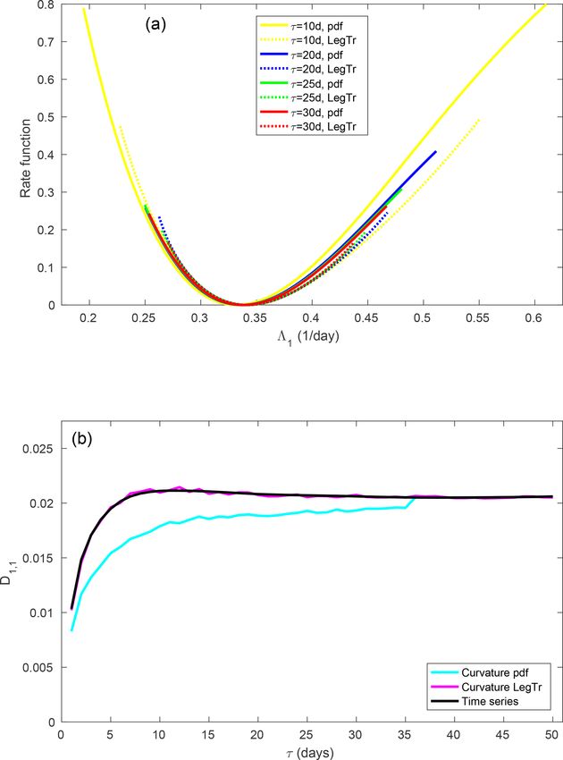
F. Kwasniok: Fluctuations of finite-time Lyapunov exponents                                                                     201

where D denotes the K × K part of the diffusion matrix cor-         moment generating function estimated as the sample mean
responding to the K retained FTLEs. A second-order Taylor           over the time series:
expansion of the joint rate function in the vicinity of λ,          D T (τ ) E 1 L−1
                                                                                 X T (τ )
       1                                                             eθ 3 =          e θ 3α .                                   (52)
I (z) ≈ (z − λ)T Q(z − λ),                                  (46)               L α=0
       2
                                                                    Again, this is a convex optimization problem and rate func-
corresponds to a multivariate Gaussian probability density
                                                                    tions obtained from the Legendre transform method are guar-
with mean λ and covariance matrix (τ Q)−1 , recovering the
                                                                    anteed to be strictly convex with a unique zero and minimum
central limit theorem (CLT).
                                                                    at z∗ = λ.
5.5     Estimating the joint rate function
                                                                    5.6    Estimating the diffusion matrix
There are again two ways of estimating the joint rate func-
                                                                    The diffusion matrix D (or the part of it corresponding to
tion from the time series of FTLEs: via the probability den-
                                                                    the K considered FTLEs) can be obtained from both joint
sity function (cf., Eq. 43) or via the Legendre transform (cf.,
                                                                    rate function estimates as the inverse of the Hessian matrix
Eq. 44).
                                                                    at the minimum (cf., Eq. 45). It can also be estimated directly
5.5.1    Probability density function approach                      from the time series of the FTLEs as given in Eq. (17). The
                                                                    estimates from the Legendre transform-based joint rate func-
By inverting Eq. (43) we get                                        tion and from the time series are always the same, apart from
                                                                    errors in the finite-difference approximation of the second
                1
                                                                    derivatives. The diffusion matrix estimates from the proba-
I (z) = − lim     log p 3(τ ) = z .                         (47)
           τ →∞ τ                                                   bility density-based joint rate function and from the time se-
                                                                    ries are the same if the model in Eq. (50) is a multivariate
The probability density of 3(τ ) is modelled as
                                                                    Gaussian probability density; otherwise they are different.
            1       h           i                                    The different methods for estimating the rate function and
p 3(τ ) = z = (τ ) exp −U (τ ) (z)                          (48)    the diffusion matrix in the univariate and the multivariate
             Z
                                                                    case are summarized in Tables 4 and 5.
with normalization constant                                            In high-dimensional systems it is usually too ambitious a
                                                                    task to determine I (z) beyond the Gaussian approximation
       Z     h          i
Z = exp −U (τ ) (z) d K z.
 (τ )
                                                            (49)    for the full system. Here, we restrict ourselves to the bivariate
         RK                                                         case K = 2.

The potential function U (τ ) (z) is expanded into suitable
multinomial basis functions as                                      6     Results
               J
               X      (τ )                                          6.1    Lyapunov exponents
U (τ ) (z) =         βi φi (z)                              (50)
               i=1                                                  Time series of FTLEs of the QG model of length L = 25 000
subject to appropriate conditions to ensure a normalizable          with a basic integration time 1τ = 1 d are generated as de-
                                                   (τ )
probability density. The expansion coefficients {βi }Ji=1 are       scribed in Sect. 3. The (global) LEs are calculated as
                                                     ) L−1
determined from the time series of the FTLEs {3(τ α }α=0 via               1 L−1
                                                                             X (1τ )
maximum likelihood which is a convex optimization prob-             λj =         3   .                                          (53)
lem with a unique solution.                                                L α=0 j,α
  The estimate of the joint rate function is
                                                                       Figure 1 displays the Lyapunov spectrum of the QG
            1 h (τ )               i
                                                                    model. There are 91 positive LEs. The largest LE is estimated
I (z) = lim    U (z) − U (τ ) (z∗ ) ,                       (51)
       τ →∞ τ                                                       as λ1 = 0.342 d−1 , corresponding to an e-folding time of per-
where z∗ denotes the position of the minimum of the po-             turbation growth of 2.9 d which appears to be realistic for the
tential function U (τ ) (z) which for finite τ is not necessarily   real atmosphere. The spectrum starts off quite steep and then
equal to λ.                                                         flattens at the near-zero exponents. For example, there are
                                                                    69 LEs between 0.05 and −0.05 d−1 . The spectrum becomes
5.5.2    Legendre transform approach                                steeper again at the trailing very stable exponents. Overall,
                                                                    there is a continuous spectrum of timescales with no clear
Alternatively, the joint rate function I (z) can be determined      timescale separation. This is in accordance with previous re-
via the multivariate Legendre transform of Eq. (44) with the        sults for QG models (Vannitsem and Nicolis, 1997; Schubert

www.nonlin-processes-geophys.net/26/195/2019/                                   Nonlin. Processes Geophys., 26, 195–209, 2019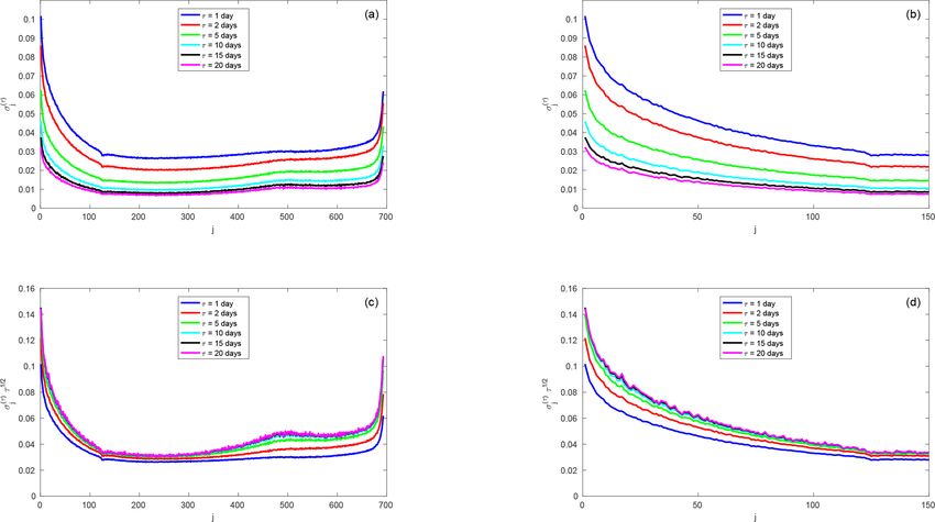
202                                                                      F. Kwasniok: Fluctuations of finite-time Lyapunov exponents

Table 4. Methods for estimating the rate function.

                              Probability density                                Legendre transform
                                              h                i                                                       (τ )

               Univariate
                                                  (τ )  (τ )
                              Ij (z) = lim τ1 Uj (z) − Uj (z∗ )                  Ij (z) = lim τ1 sup θz − log L1 PL−1 eθ3j,α
                                        τ →∞                                             τ →∞                     α=0
                                                                                               θ ∈R
                                                                                                                1 PL−1 eθ T3(τ )
                                                h                        i                             h                          i
               Multivariate   I (z) = lim τ1 U (τ ) (z) − U (τ ) (z∗ )           I (z) = lim τ1 sup θ T z − log L  α=0
                                                                                                                            α
                                     τ →∞                                               τ →∞
                                                                                               θ ∈RK

Table 5. Methods for estimating the diffusion matrix.

                        Probability density           Legendre transform                 Time series
                                                                                                      PL−1  (τ )     2
                         −1                            −1                                           τ
         Univariate     Dj,j = Ij00 (z∗ )             Dj,j = Ij00 (λj )                  Dj,j = lim L  α=0 3j,α − λj
                                                                                               τ →∞
                                            2                                2

         Multivariate   (D−1 )j,k = ∂z∂ ∂z
                                        I             (D−1 )j,k = ∂z∂ ∂z
                                                                      I                             τ PL−1 3(τ ) − λ
                                                                                         Dj,k = lim L                    3
                                                                                                                          (τ )
                                                                                                                               − λ
                                       j k z=z∗                      j k z=λ                   τ →∞    α=0   j,α    j     k,α      k

                                                                                 increase again towards the end of the Lyapunov spectrum
                                                                                 with a particularly sharp increase for the most stable expo-
                                                                                 nents at the very end of the spectrum. This is in line with sim-
                                                                                 ilar findings in simple spatially extended systems (Kuptsov
                                                                                 and Politi, 2011; Pazó et al., 2013) as well as in a QG
                                                                                 atmosphere–ocean model (Vannitsem and Lucarini, 2016).
                                                                                                                       (τ )
                                                                                    The scaled standard deviation σj τ 1/2 shows clear con-
                                                                                 vergence for all of the exponents at τ = 10–15 d, that is to
                                                                                 say the scaled variance converges to the diagonal elements
                                                                                 Dj,j of the diffusion matrix D. Convergence is reached at
                                                                                 about τ = 10 d for almost all of the exponents; it is particu-
                                                                                 larly fast for the near-neutral and the weakly dissipative ex-
                                                                                 ponents where it is already reached at τ = 5–10 d.
                                                                                    There is a kink-like feature at j ≈ 125, separating regions
                                                                                 with different slopes of the standard deviation. It is possible
                                                                                 that this is linked to a distinction of the covariant Lyapunov
                                                                                 vectors into interacting “physical modes” and hyperbolically
                                                                                 separated “isolated modes” (Yang et al., 2009). But this cer-
                                                                                 tainly needs further investigation.

                                                                                 6.2   Multivariate fluctuation analysis

                                                                                 Figure 3 shows the explained variance and the cumulative
                                                                                 explained variance of the principal components of the scaled
                                                                                 Lyapunov fluctuations. There are three leading modes, then
Figure 1. (a) Lyapunov spectrum of the QG model. (b) Close-up                    the eigenvalue spectrum sharply flattens off. The fraction of
of (a).
                                                                                 variance explained by the leading modes increases with in-
                                                                                 creasing integration time τ . Going from τ = 1 to τ = 20 d,
                                                                                 the variance explained by the first principal component in-
and Lucarini, 2015) and is probably because QG equations                         creases from just below 5 % to more than 12 %, and the vari-
are scale-filtered equations.                                                    ance explained by the second principal component increases
                                           (τ )
   Figure 2 shows the standard deviation σj of the fluctu-                       from about 2 % to more than 4 %. However, due to the flat-
ations of the FTLEs around their mean values (Eq. 40). The                       ness of the bulk of the eigenvalue spectrum, even in the dif-
standard deviation monotonically decreases with increasing                       fusion limit a substantial number of modes is necessary to
integration time τ for all exponents. The fluctuations are                       explain large parts of the fluctuation variance. The eigen-
largest for the leading LEs and then quickly decrease. They                      value spectrum is still not fully converged at τ = 20 d. It is

Nonlin. Processes Geophys., 26, 195–209, 2019                                              www.nonlin-processes-geophys.net/26/195/2019/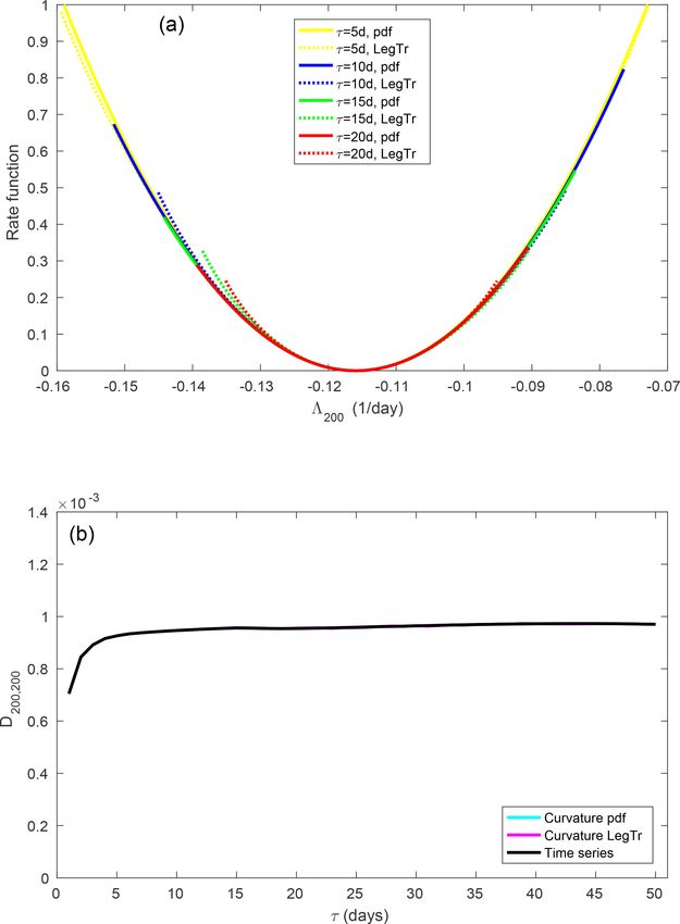
F. Kwasniok: Fluctuations of finite-time Lyapunov exponents                                                                              203

                                   (τ )                                                                    (τ )
Figure 2. (a) Standard deviation σj       of the FTLEs. (b) Close-up of (a). (c) Scaled standard deviation σj τ 1/2 of the FTLEs. (d) Close-up
of (c).

Figure 3. (a) Variance of the principal components of the finite-time Lyapunov fluctuations. (b) Fraction of variance. (c) Cumulative fraction
of variance. (d) Close-up of (c).

www.nonlin-processes-geophys.net/26/195/2019/                                           Nonlin. Processes Geophys., 26, 195–209, 2019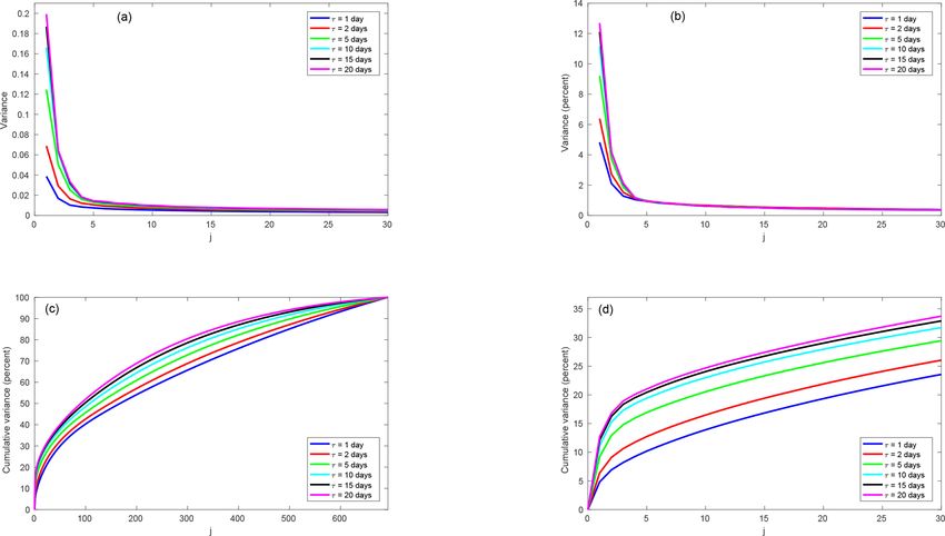
204                                                                  F. Kwasniok: Fluctuations of finite-time Lyapunov exponents

                                                                                                             (τ )        (τ )
                                                                         Figure 5. Correlation of the FTLEs 3j      and 3k      for (a) τ = 1 d
                                                                         and (b) τ = 15 d.

                                                                         Lyapunov spectrum. In the second EOF, the leading FTLEs
                                                                         again fluctuate in phase; here, this encompasses about the
Figure 4. (a) First, (b) second and (c) third normalized empirical       first 40 exponents. Then there is some negative correlation
orthogonal function (EOF) of the finite-time Lyapunov fluctuations       with the weakly dissipative exponents and substantial pos-
(cf., Eq. 20).                                                           itive correlation with the strongly dissipative exponents at
                                                                         the end of the Lyapunov spectrum. The third EOF has the
                                                                         very stable exponents at the end of the spectrum fluctuating
not completely clear what the reason for this is. There may              in phase and the most unstable exponents fluctuating in phase
be some indication that the off-diagonal elements of the dif-            with each other, out of phase with the dissipative ones.
fusion matrix converge slightly more slowly than the diago-                 Complementary to the EOF analysis, Fig. 5 shows the cor-
nal elements. But there is probably also a finite sample size            relation of selected FTLEs with each of the other FTLEs for
effect. With increasing τ , the time series of the FTLEs con-            τ = 1 and τ = 15 d. The pattern of the correlations is the
tain less and less uncorrelated information and fail to fully            same for both integration times but the amplitudes are very
sample the high-dimensional covariance matrix which leads                low for τ = 1 d and build up at larger integration times. This
to an overestimation of the variance of the leading principal            is in line with the results from the EOF analysis. The FTLEs
components.                                                              have predominantly positive correlations with neighbouring
   In Fig. 4 the three leading EOFs are displayed. The modes             exponents; these are strongest for the most unstable and the
are largely independent of the integration time τ and have               most stable exponents and weaker in between. There are also
converged at about τ = 10 d. The first EOF shows a pattern               some relatively weak long-range correlations across the Lya-
where all of the leading FTLEs fluctuate in phase. This in-              punov spectrum.
corporates all of the positive exponents and extends to the
weakly dissipative ones. Then there is some negative corre-
lation with the dissipative exponents in the second half of the

Nonlin. Processes Geophys., 26, 195–209, 2019                                     www.nonlin-processes-geophys.net/26/195/2019/
F. Kwasniok: Fluctuations of finite-time Lyapunov exponents 205
Figure 6. Order of the model for the probability density function of
(τ )
the FTLE 3j .
6.3 Large-deviation analysis
6.3.1 One-dimensional approach
We now investigate whether the fluctuations of the FTLEs
obey a large deviation principle. As representative examples
we look at the first and the fifth exponent as two strongly
unstable modes, at the zero exponent, at a weakly dissi-
pative exponent and at the smallest, most stable exponent.
The large-deviation rate function is estimated as described
in Sect. 5 from the probability density function and via the
Legendre transform for various values of τ . The correspond-
ing element Dj,j of the diffusion matrix is calculated from
the curvature of the two estimates of the rate function and
directly from the time series of the FTLEs. Figure 7. (a) Large-deviation rate function of the first FTLE. (b) El-
To model the probability density of the FTLEs two dif- ement D1,1 of the diffusion matrix.
ferent choices for the potential function in Eq. (39) are
considered here: M = 2, this is to say a Gaussian prob-
ability density, and M = 4, a fourth-order polynomial. In even more pronounced than those for the first exponent and
view of the high degree of correlation in the time series detectable up to an integration time as large as τ = 49 d. For
of the FTLEs, particularly for large τ , model selection the first and the last exponent, at small integration times τ
is performed here as follows. For τ = n1τ , the time se- it may be possible to even switch to the higher-order model
(τ )
ries of the FTLEs, {3j,α }L−1 α=0 , are sub-sampled into n dis- M = 6 but this is not our concern here.
joint time series with non-overlapping integration time inter- Figure 7 shows the results of the large-deviation analysis
(τ ) (τ ) (τ )
vals, {3j,m , 3j,m+n , 3j,m+2n , . . .}, for m = 0, . . ., n − 1. The for the first FTLE. Convergence to a large-deviation princi-
length of the sub-sampled time series is the largest integer L0 ple is observed. At τ = 10 d and even visible at τ = 20 d the
such that m + (L0 − 1)n ≤ L − 1. The two probability den- maximum of the probability density is still shifted away from
sity models are fitted separately on the n sub-sampled time the mean; nevertheless, some convergence among the proba-
series and model selection is based on the average Bayesian bility density-based estimates of the rate function is reached
information criterion. Then the selected model is fitted on the at about τ = 20 d. The Legendre transform-based estimates
whole time series. already give a consistent picture from τ = 10 d. Good con-
Figure 6 displays the order of the model for the probability vergence is also observed for the corresponding element of
density of the selected FTLEs as a function of the integra- the diffusion matrix.
tion time τ . The leading unstable exponents exhibit strong For the fifth FTLE, a similar picture can be seen (Fig. 8)
non-Gaussianity. For the first exponent, it is detectable up to but convergence is markedly faster than for the first FTLE.
τ = 35 d; for the fifth exponent, it is less pronounced and vis- The probability density-based estimates are very consistent
ible only up to τ = 12 d. The zero exponent shows only very from τ = 10–15 d; note that the model for the probability
mild non-Gaussianity which is visible for τ = 1 and τ = 2 d. density jumps from fourth-order to Gaussian for the higher
The weakly dissipative exponent has Gaussian behaviour at values of τ . The Legendre transform already gives close
all values of τ . The smallest, strongly dissipative exponent agreement for the rate function from τ = 5 d.
again displays marked deviations from Gaussianity; these are
www.nonlin-processes-geophys.net/26/195/2019/ Nonlin. Processes Geophys., 26, 195–209, 2019206 F. Kwasniok: Fluctuations of finite-time Lyapunov exponents
Figure 8. (a) Large-deviation rate function of the fifth FTLE. (b) El-
ement D5,5 of the diffusion matrix. Figure 9. (a) Large-deviation rate function of the 92th FTLE.
(b) Element D92,92 of the diffusion matrix.
For the zero exponent (Fig. 9), convergence is again Table 6. Correlation length lj
(1τ )
of the time series of the FTLE
markedly faster than for both positive exponents. A large- (1τ )
3j with 1τ = 1 d.
deviation principle can already be established from about
τ = 10 d, and the two different estimates of the rate function
are close together. The estimates of the diffusion coefficient j 1 5 92 200 693
all coincide. (1τ )
lj 2.07 2.10 1.61 1.38 3.25
For the fully Gaussian 200th FTLE (Fig. 10), convergence
is even faster. A large-deviation principle is valid from τ =
5 d and all of the estimates of the rate function are in almost (τ )
perfect agreement. The estimates of the diffusion coefficient FTLEs. The correlation length of the FTLE 3j is defined
show corresponding behaviour. as
For the smallest, most dissipative exponent (Fig. 11), the ∞
(τ ) (τ )
X
convergence to a large-deviation principle is very slow, even lj = 1 + 2 ρj,i , (54)
slower than for the first, most unstable exponent. A large- i=1
deviation principle is valid from about τ = 30 d, and the Leg- (τ ) (τ )
endre transform method gives reliable estimates of the rate where ρj,i is the autocorrelation of the FTLE 3j at
function from τ = 10 to 20 d. Also, the convergence of the lag i. Note that a lag of 1 here refers to two consecu-
diffusion coefficient is markedly slow. The estimate from the tive but non-overlapping integration time intervals of length
(τ )
non-Gaussian probability density is initially too low and con- τ , that is to say ρj,i is the autocorrelation at lag i of
(τ )
verges at about τ = 25 d. the sub-sampled time series of 3j as introduced above
The different speeds of convergence to a large-deviation for the model selection of the probability density model,
(τ ) (τ ) (τ )
principle for the different FTLEs can be understood from {3j,m , 3j,m+n , 3j,m+2n , . . .}, for m = 0, 1, . . ., n − 1. There
the degrees of serial correlation and non-Gaussianity of the are n of these which can be used to generate n estimates of
Nonlin. Processes Geophys., 26, 195–209, 2019 www.nonlin-processes-geophys.net/26/195/2019/F. Kwasniok: Fluctuations of finite-time Lyapunov exponents 207
Figure 10. (a) Large-deviation rate function of the 200th FTLE. Figure 11. (a) Large-deviation rate function of the 693th FTLE.
(b) Element D200,200 of the diffusion matrix. (b) Element D693,693 of the diffusion matrix.
fusion limit and convergence occurs immediately after cor-
(τ )
lj and then take the average. The definition of the corre- relation decay; otherwise it is further delayed, generally the
lation length of Eq. (54) occurs naturally in the formulation longer the delay the larger the departure from Gaussianity.
of the CLT for dependent random variables (e.g. Billings- Table 6 gives the correlation length of the selected FTLEs
(1τ ) (1τ )
ley, 1995) under the assumption of a Markov process that 3j at the basic integration time 1τ = 1 d. Note that lj
is sufficiently mixing. Now consider two integration times does not allow one to directly calculate the value of τ at
τ1 = n1 1τ and τ2 = n2 1τ with n1 ≤ n2 and n0 = n2 /n1 be- which convergence to a large-deviation principle occurs but
ing an integer for simplicity; one could consider a continu- it gives an impression of the timescales of temporal correla-
ous integration time τ in the limit 1τ → 0. The variances of tion and how they differ for the different FTLEs. Overall,
(τ ) 2 (τ ) 2 (τ )
h i h i
(τ ) (τ )
3j 1 and 3j 2 are linked as σj 2 = σj 1 lj 1 /n0 , and temporal correlation is not very pronounced for all of the
FTLEs, but the correlation length varies by a factor of 2.35
the two estimates of the diffusion coefficient, as calculated
from the shortest to the longest. The rapid convergence to a
from the time series or the Legendre transform, are linked as
(τ ) (τ ) (τ ) large-deviation principle for the zero and weakly dissipative
Dj,j2 = Dj,j1 lj 1 . This holds in the limit n0 → ∞, otherwise
exponents is in line with their short correlation length and
(τ )
lj 1 needs to be replaced with a counterpart that takes only almost Gaussian distribution. For the first and the last expo-
a finite number of lags into account and also contains some nent convergence is delayed beyond what is expected from
correction terms. Convergence to a large-deviation principle the somewhat larger correlation length due to the strong non-
is limited by serial correlation of the FTLEs. Convergence to Gaussianity .
the diffusion limit, that is to the Gaussian approximation of
the large-deviation regime, can certainly not be expected be- 6.3.2 Two-dimensional approach
fore the serial correlations have decayed, that is to say when
(τ )
lj ≈ 1. If the distribution of the FTLEs is Gaussian or close As an example of a multivariate large-deviation analysis,
to Gaussian the large-deviation limit is equivalent to the dif- Fig. 12 shows the joint large-deviation rate function of the
www.nonlin-processes-geophys.net/26/195/2019/ Nonlin. Processes Geophys., 26, 195–209, 2019208 F. Kwasniok: Fluctuations of finite-time Lyapunov exponents
Figure 12. Joint large-deviation rate function of the first two FTLEs as estimated from the joint probability density for (a) τ = 10 d, (b) τ =
15 d and (c) τ = 25 d; and with the Legendre transform for (d) τ = 10 d, (e) τ = 15 d and (f) τ = 25 d. Black dots indicate the global LEs
(λ1 , λ2 ); and red dots in panels (a), (b) and (c) indicate the maximum of the joint probability density. (g) Elements D1,1 (solid), D2,2
(dashed) and D1,2 (dotted) of the diffusion matrix as estimated from the curvature of the probability density-based rate function (cyan), from
the curvature of the Legendre transform-based rate function (magenta) and from the time series of the FTLEs (black).
first two FTLEs, 31 and 32 . The estimates of the diffusion 7 Conclusions
coefficients D1,1 , D2,2 and D1,2 are also shown. The poten-
tial function for the joint probability density is chosen as The statistical properties of the fluctuations of FTLEs were
!i−j !j investigated in a three-level quasi-geostrophic atmospheric
M X
i model with realistic mean state and variability. The Lya-
X (τ ) z 1 − λ1 z2 − λ2
U (τ ) (z1 , z2 ) = βi,j (τ ) (τ )
, punov spectrum of the model has almost 100 positive LEs
i=1 j =0 σ1 σ2
and displays no clear timescale separation.
(55) A principal component analysis of the fluctuations of the
FTLEs around their mean values was performed. The scaled
where the order of the model is fixed a priori at M = 4. covariance matrix of the fluctuations is converged to the lim-
The joint rate function displays markedly non-Gaussian be- iting diffusion matrix at about τ = 15 d. There are substantial
(τ ) (τ )
haviour and some dependence between 31 and 32 . Con- correlations among the different FTLEs. The first three em-
vergence to a large-deviation principle is mainly reached at pirical orthogonal functions are patterns where the leading
τ = 15 d, as can be seen from the probability density-based positive FTLEs fluctuate together in phase. These modes are
estimates of the joint rate function. The estimates from the largely independent of the integration time τ .
Legendre transform are in agreement and already indicate the A large-deviation principle can be established for all of
joint rate function at τ = 10 d. The elements of the diffusion the FTLEs. The convergence to the large-deviation limit is
matrix are well estimated overall with detailed convergence slightly slow for the most unstable and the most stable FTLEs
being somewhat slow in accordance with the univariate anal- and very fast in between. Convergence to the diffusion limit,
ysis for the first FTLE. The estimate of the off-diagonal ele- that is to the Gaussian approximation of the large-deviation
ment D1,2 is particularly good. regime, is generally faster. Also a joint large-deviation rate
function for the first and the second FTLE was successfully
estimated beyond the Gaussian approximation. Good corre-
spondence was found between the curvature of the rate func-
tions at the minimum and the corresponding elements of the
diffusion matrix.
Nonlin. Processes Geophys., 26, 195–209, 2019 www.nonlin-processes-geophys.net/26/195/2019/F. Kwasniok: Fluctuations of finite-time Lyapunov exponents 209
Two different methods for estimating the large-deviation Kifer, Y.: Large deviations in dynamical systems and stochastic pro-
rate functions from the data were discussed: an approach cesses, T. Am. Math. Soc., 321, 505–524, 1990.
via the probability density function and an approach using Kuptsov, P. V. and Parlitz, U.: Theory and computation of covariant
the Legendre transform. The Legendre transform method ap- Lyapunov vectors, J. Nonlinear Sci., 22, 727–762, 2012.
pears to be generally superior for finding the rate function Kuptsov, P. V. and Politi, A.: Large-deviation approach
to space-time chaos, Phys. Rev.Lett., 107, 114101,
as (i) convergence occurs at a smaller value of the integra-
https://doi.org/10.1103/PhysRevLett.107.114101, 2011.
tion time τ where more independent data are available and Kwasniok, F.: Reduced atmospheric models using dynamically mo-
(ii) it yields diffusion coefficients fully consistent with their tivated basis functions, J. Atmos. Sci., 64, 3452–3474, 2007.
direct estimation from the data. Nevertheless, both methods Laffargue, T., Lam, K.-D. N. T., Kurchan, J., and Tailleur, J.: Large
should be considered side by side as the probability density deviations of Lyapunov exponents, J. Phys. A-Math. Theor., 46,
approach allows one to monitor if/when the probability den- 254002, https://doi.org/10.1088/1751-8113/46/25/254002, 2013.
sity function has actually reached the large-deviation regime. Legras, B., and Ghil, M.: Persistent Anomalies, Blocking, and Vari-
ations in Atmospheric Predictability, J. Atmos. Sci., 42, 433–471,
1985.
Data availability. The data and codes relating to this paper are Lorenz, E. N.: Deterministic Nonperiodic Flow, J. Atmos. Sci., 20,
available upon request from the author. They are not publicly ac- 130–141, 1963.
cessible, as they were created solely for the purpose of this research Marshall, J. and Molteni, F.: Toward a dynamical understanding
study. of planetary-scale flow regimes, J. Atmos. Sci., 50, 1792–1818,
1993.
Oseledets, V. I.: A multiplicative ergodic theorem, Characteristic
Competing interests. The author declares that they have no conflict Ljapunov exponents of dynamical systems, Transactions of the
of interest. Moscow Mathematical Society, 19, 179–210, 1968.
Ott, E.: Chaos in Dynamical Systems, Cambridge University Press,
Cambridge, 2002.
Pazó, D., López, J. M., and Politi, A.: Universal scaling of
Special issue statement. This article is part of the special is-
Lyapunov-exponent fluctuations in space-time chaos, Phys. Rev.
sue “Numerical modeling, predictability and data assimilation in
E, 87, 062909, https://doi.org/10.1103/PhysRevE.87.062909,
weather, ocean and climate: A special issue honoring the legacy of
2013.
Anna Trevisan (1946–2016)”. It is not associated with a conference.
Pikovsky, A. and Politi, A.: Lyapunov Exponents, Cambridge Uni-
versity Press, Cambridge, 2016.
Roads, J. O.: Predictability in the extended range, J. Atmos. Sci.,
Acknowledgements. The author would like to thank the three 44, 3495–3527, 1987.
anonymous reviewers for their comments which helped improve the Rohwer, C. M., Angeletti, F., and Touchette, H.: Convergence
presentation and clarity of the paper. of large-deviation estimators, Phys. Rev. E, 92, 052104,
https://doi.org/10.1103/PhysRevE.92.052104, 2015.
Schubert, S. and Lucarini, V.: Covariant Lyapunov vectors of a
Review statement. This paper was edited by Juan Manuel Lopez quasi-geostrophic baroclinic model: Analysis of instabilities and
and reviewed by three anonymous referees. feedbacks, Q. J. Roy. Meteorol. Soc., 141, 3040–3055, 2015.
Shimada, I. and Nagashima, T.: A Numerical Approach to Ergodic
Problem of Dissipative Dynamical Systems, Prog. Theor. Phys.,
61, 1605–1616, 1979.
Touchette, H.: The large deviation approach to statistical mechanics,
References Phys. Rep., 478, 1–69, 2009.
Vannitsem, S.: Predictability of large-scale atmospheric motions:
Benettin, G., Galgani, L., Giorgilli, A., and Strelcyn, J.-M.: Lya- Lyapunov exponents and error dynamics, Chaos, 27, 032101,
punov characteristic exponents for smooth dynamical systems https://doi.org/10.1063/1.4979042, 2017.
and for Hamiltonian systems: a method for computing all of Vannitsem, S. and Lucarini, V.: Statistical and Dynamical Proper-
them, Part 1: Theory, Meccanica, 15, 9–20, 1980. ties of Covariant Lyapunov Vectors in a Coupled Atmosphere-
Billingsley, P.: Probability and Measure, 3rd edn., Wiley, New York, Ocean Model – Multiscale Effects, Geometric Degeneracy,
1995. and Error Dynamics, J. Phys. A-Math. Theor., 49, 224001,
Eckmann, J. and Ruelle, D.: Ergodic theory of chaos and strange https://doi.org/10.1088/1751-8113/49/22/224001, 2016.
attractors, Rev. Mod. Phys., 57, 617–656, 1985. Vannitsem, S. and Nicolis, C.: Lyapunov Vectors and Error Growth
Ehrendorfer, M.: The total energy norm in a quasigeostrophic Patterns in a T21L3 Quasigeostrophic Model, J. Atmos. Sci., 54,
model, J. Atmos. Sci., 57, 3443–3451, 2000. 347–361, 1997.
Johnson, P. L. and Meneveau, C.: Large-deviation joint statistics of Yang, H.-L., Takeuchi, K. A., Ginelli, F., Chaté, H., and Radons,
the finite-time Lyapunov spectrum in isotropic turbulence, Phys. G.: Hyperbolicity and the Effective Dimension of Spatially
Fluids, 27, 085110, https://doi.org/10.1063/1.4928699, 2015. Extended Dissipative Systems, Phys. Rev. Lett., 102, 074102,
Kalnay, E.: Atmospheric Modeling, Data Assimilation, and Pre- https://doi.org/10.1103/PhysRevLett.102.074102, 2009.
dictability, Cambridge University Press, Cambridge, 2003.
www.nonlin-processes-geophys.net/26/195/2019/ Nonlin. Processes Geophys., 26, 195–209, 2019You can also read