The Increased Likelihood in the 21st Century for a Tropical Cyclone to Rapidly Intensify When Crossing a Warm Ocean Feature-A Simple Model's ...

Page created by Jeanne Hart
 
CONTINUE READING
The Increased Likelihood in the 21st Century for a Tropical Cyclone to Rapidly Intensify When Crossing a Warm Ocean Feature-A Simple Model's ...
atmosphere

Article
The Increased Likelihood in the 21st Century for a Tropical
Cyclone to Rapidly Intensify When Crossing a Warm Ocean
Feature—A Simple Model’s Prediction
Leo Oey

                                          Forrestal Campus, Princeton University, Princeton, NJ 08544, USA; lyo@alumni.princeton.edu

                                          Abstract: A warm ocean feature (WOF) is a blob of the ocean’s surface where the sea-surface
                                          temperature (SST) is anomalously warmer than its adjacent ambient SST. Examples are warm coastal
                                          seas in summer, western boundary currents, and warm eddies. Several studies have suggested that
                                          a WOF may cause a crossing tropical cyclone (TC) to undergo rapid intensification (RI). However,
                                          testing the “WOF-induced RI” hypothesis is difficult due to many other contributing factors that can
                                          cause RI. The author develops a simple analytical model with ocean feedback to estimate TC rapid
                                          intensity change across a WOF. It shows that WOF-induced RI is unlikely in the present climate when
                                          the ambient SST is .29.5 ◦ C and the WOF anomaly is .+1 ◦ C. This conclusion agrees well with the
                                          result of a recent numerical ensemble experiment. However, the simple model also indicates that
                                          RI is very sensitive to the WOF anomaly, much more so than the ambient SST. Thus, as coastal seas
         
                                   and western boundary currents are warming more rapidly than the adjacent open oceans, the model
Citation: Oey, L. The Increased
                                          suggests a potentially increased likelihood in the 21st century of WOF-induced RIs across coastal
Likelihood in the 21st Century for a      seas and western boundary currents. Particularly vulnerable are China’s and Japan’s coasts, where
Tropical Cyclone to Rapidly Intensify     WOF-induced RI events may become more common.
When Crossing a Warm Ocean
Feature—A Simple Model’s                  Keywords: rapid intensification; typhoons; tropical cyclones; warm ocean features; coastal seas;
Prediction. Atmosphere 2021, 12, 1285.    western boundary currents; warm eddies; western North Pacific; China and Japan coasts
https://doi.org/10.3390/
atmos12101285

Academic Editors: Ziqian Wang,            1. Introduction
Lin Chen, Shang-Min Long and
                                               A tropical cyclone (TC) is said to undergo rapid intensification (RI) when its maximum
Gen Li
                                          10-m wind increases by more than 15.4 m/s in 1 day [1]. RI may be due to TC internal
Received: 19 August 2021
                                          dynamics, environmental factors, and a combination [2–16]. Often, storms that have
Accepted: 30 September 2021
                                          undergone RI develop into major storms (Category 3 and above) [17,18]. They are therefore
Published: 2 October 2021                 of interest to researchers and forecasters.
                                               By supplying heat and moisture to the atmosphere, ocean, and coupled ocean feed-
Publisher’s Note: MDPI stays neutral      back play a significant role in TC intensity change [19–21]. Some studies suggested that
with regard to jurisdictional claims in   RI may be triggered when a TC crosses a warm ocean feature (WOF) [12,22–29]. The
published maps and institutional affil-   WOF may be a warm eddy, a western boundary current, or a summertime coastal shelf
iations.                                  sea. It has an anomalously warmer sea-surface temperature (SST) than the ambient sea.
                                          We define WOF-induced RI when the RI triggered as a TC crosses a WOF. In practice,
                                          however, isolating and identifying WOF-induced RI is challenging due to the simultaneous
                                          existence of other factors cited above. Oey and Huang [30] designed numerical ensemble
Copyright: © 2021 by the author.
                                          experiments to eliminate other potential RI-causing environmental factors and isolate the
Licensee MDPI, Basel, Switzerland.        WOF-induced intensity change. They conducted twin experiments and showed statistically
This article is an open access article    indistinguishable RI occurrences between the experiments with and without the WOF.
distributed under the terms and           They then used a strip-down version of the analytical model presented here to support
conditions of the Creative Commons        their numerical findings.
Attribution (CC BY) license (https://          In this manuscript, we extend and provide complete details of the analytical model.
creativecommons.org/licenses/by/          The analytical model includes ocean feedback and estimates the WOF-induced intensity
4.0/).

Atmosphere 2021, 12, 1285. https://doi.org/10.3390/atmos12101285                                       https://www.mdpi.com/journal/atmosphere
The Increased Likelihood in the 21st Century for a Tropical Cyclone to Rapidly Intensify When Crossing a Warm Ocean Feature-A Simple Model's ...
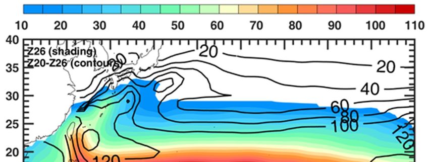
Atmosphere 2021, 12, x FOR PEER REVIEW                                                                                                      2 of 15

Atmosphere 2021, 12, 1285                                                                                                      2 of 15
                                        In this manuscript, we extend and provide complete details of the analytical model.
                                  The analytical model includes ocean feedback and estimates the WOF‐induced intensity
                                  change and RI. The model shows that ocean feedback decreases intensity change, neces‐
                                  sitatingand
                                 change     a warmer
                                                RI. TheWOF
                                                         modelanomaly    for ocean
                                                                shows that   a TC to    developdecreases
                                                                                     feedback     RI. We provide    observations
                                                                                                            intensity             and
                                                                                                                      change, neces-
                                  conclude    that WOF‐induced     RI is unlikely   under  the present   background
                                 sitating a warmer WOF anomaly for a TC to develop RI. We provide observations and     and WOF   SSTs
                                  in the tropics
                                 conclude          and subtropics.
                                             that WOF-induced      RIHowever,
                                                                     is unlikelyWOFs
                                                                                   undercan
                                                                                          the potentially   play an increasingly
                                                                                              present background      and WOF SSTssig‐
                                  nificant
                                 in         role in
                                    the tropics     triggering
                                                  and           RIsHowever,
                                                       subtropics.  as these SSTs,
                                                                              WOFs   particularly   the WOF
                                                                                       can potentially   play SST, continue tosignif-
                                                                                                              an increasingly  rise in
                                  a warming
                                 icant  role in climate.
                                                triggering RIs as these SSTs, particularly the WOF SST, continue to rise in a
                                 warming climate.
                                  2. The Model
                                 2. The Model
                                  2.1. The Problem
                                 2.1. The Problem
                                        A tropical cyclone (TC) translates westward along the negative x-axis at a constant
                                  speedAU tropical  cyclone (TC) translates westward along the negative x-axis at a constant
                                            h. Across x = 0, the SST (T) changes by δTW due to a WOF:
                                 speed Uh . Across x = 0, the SST (T) changes by δTW due to a WOF:
                                                                         T = To              x ≥ 0,
                                                                      T = T0               x ≥ 0,                                   (1)
                                                                                                                                  (1)
                                                                          == T
                                                                             To0 ++δT
                                                                                    δTWw x < x > 0.0. We
                                                                                            We focus
                                                                                                   focus onon the
                                                                                                               the redpoint
                                                                                                                    redpointshortly
                                                                                                                               shortlyafter
                                                                                                                                          afterthe
                                                                                                                                                 the
                                 crossing    under     the  direct  path of the storm’s   core  or  eyewall,   where
                                   crossing under the direct path of the storm's core or eyewall, where SST changes,   SST  changes,    and  ocean
                                                                                                                                                and
                                 feedback      can mostcan
                                   ocean feedback           influence   intensity [19,31,32].
                                                                 most influence     intensity The      goal is to
                                                                                                  [19,31,32].     calculate
                                                                                                                The   goal isthetochange     in the
                                                                                                                                     calculate   the
                                 maximum          wind
                                   change in the maximum (δV  m ) and  estimate  the  (δT   ,
                                                                       wind (δVm) andWestimateT 0 )-combination     where   a WOF-induced
                                                                                                        the (δTW, To)‐combination where          RIa
                                 isWOF‐induced
                                    possible. The analysis         is independent
                                                        RI is possible.              of where
                                                                          The analysis           the redpointofis,where
                                                                                          is independent            provided    it is in theis,
                                                                                                                           the redpoint       WOF
                                                                                                                                                pro‐
                                 and    the direct    path   of the  storm’s  core.
                                   vided it is in the WOF and the direct path of the storm’s core.

                                  Figure1.1.AAtropical
                                 Figure         tropical  cyclone
                                                       cyclone  (TC)(TC) translates
                                                                      translates    westward
                                                                                 westward        at a constant
                                                                                            at a constant       Uh across
                                                                                                          Uh across         x = 0a onto
                                                                                                                    x = 0 onto     warmaocean
                                                                                                                                          warm
                                  ocean feature
                                 feature          (WOF)SST
                                         (WOF) where       where   SST increases
                                                              increases  by δTW .by
                                                                                  TheδTcircles
                                                                                        W. The circles depict the TC wind from weak, e.g.,
                                                                                               depict the TC wind from weak, e.g., 18 m/s
                                  18the
                                 in  m/s  in the
                                        outer     outer
                                               circle    circle ofL radius
                                                      of radius            L to the maximum
                                                                    to the maximum                in the inner‐most
                                                                                      in the inner-most    ‘core’. As 'core'. As the
                                                                                                                       the storm      storm ap‐
                                                                                                                                   approaches,
                                  proaches, wind at the redpoint strengthens from weak to the maximum over a time ~ L/Uh shortly
                                 wind at the redpoint strengthens from weak to the maximum over a time ~L/Uh shortly after the
                                  after the storm crosses into the WOF. The goal is to calculate the increased wind δVm due to the
                                 storm crosses into the WOF. The goal is to calculate the increased wind δVm due to the coupled
                                  coupled response of the WOF and ocean cooling.
                                 response of the WOF and ocean cooling.
                                  2.2.Intensity
                                 2.2.  IntensityChange
                                                ChangeDue
                                                       Duetotothe
                                                               theWOF:
                                                                   WOF:The
                                                                         the WOF-Induced
                                                                             WOF-Induced RI   RI
                                        TheTC
                                       The  TCexperiences
                                                experiencesaawarmer
                                                               warmerSSTSSTasasititcrosses
                                                                                    crossesxx==0.0.The
                                                                                                    Thewarmer
                                                                                                         warmerSSTSSTincreases
                                                                                                                      increasesthe
                                                                                                                                the
                                  wind,   which  we can  estimate  using the  maximum      potential   intensity (MPI) theory
                                 wind, which we can estimate using the maximum potential intensity (MPI) theory [19]. We       [19].
                                  Wethe
                                 use   useempirical
                                           the empirical
                                                    formform
                                                          givengiven  by DeMaria
                                                                 by DeMaria          and Kaplan
                                                                              and Kaplan     [33]: [33]:
                                                                               Vm = A + B eC(T‐30).                                             (2)
                                                                             Vm = A + B eC(T-30) .                                             (2)

                                 Here, Vm (m/s) is the maximum wind, the SST T is in ◦ C, and A, B, and C are empirical
                                 coefficients. DeMaria and Kaplan [33] limit the applicability of Equation (2) to T ≤ 30 ◦ C.
                                 However, later extensions using higher-resolution data suggest no such limit [6,34,35]. The
The Increased Likelihood in the 21st Century for a Tropical Cyclone to Rapidly Intensify When Crossing a Warm Ocean Feature-A Simple Model's ...
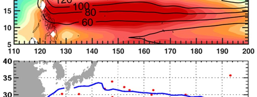
Atmosphere 2021, 12, 1285                                                                                               3 of 15

                            change in the maximum wind, δVm , due to a change in SST, δT, i.e., the WOF-induced
                            intensity change, is:
                                                                          
                                            δVm = s δT + s C δT2 /2 + 0 δT3 ; s(T) = (∂Vm /∂T) 0 ,           (3)

                            where (..)|0 means evaluation at the ambient state T0 , and s is the slope of Vm in the T-space.
                            Partial derivatives are a reminder that (A, B, C) may not depend on T alone. We assume
                            the increased intensity occurs within one day of the storm crossing x = 0 and define WOF-
                            induced RI when δVm ≥ 15.4 m/s. The vast majority (85%) of RI events occur in storms
                            that translate faster than ~3 m/s [36]. The assumption is reasonable since the time for the
                            TC core to cross a WOF of typical size 100–200 km [30] is one day or less. By definition,
                            V0 . Vm , where V0 is the maximum wind of the TC approaching the WOF. We will see that
                            δV0 . δVm (see Section 2.3.6 below). Therefore, the above RI criterion “δVm ≥ 15.4 m/s” is
                            more easily satisfied than the conventional RI criterion “δV0 ≥ 15.4 m/s”. In other words,
                            if the model predicts RI to be unlikely in the present climate, as will be shown to be the
                            case, using the conventional criterion leads to the same conclusion.

                            2.3. Ocean Feedback
                                 The increased δVm in the WOF (the red point) increases ocean mixing and up-
                            welling [37,38], hence SST cooling, δT0 < 0, which reduces δVm . The reduced δVm modifies
                            the amount of cooling, which further changes the δVm , in a coupled manner.

                            2.3.1. Assumptions
                                  We assume an ocean with no horizontal variation. For example, the SST front at x = 0
                            is fixed and has no dynamics. Vertical mixing then predominantly controls the SST cooling
                            under super-critically translating storms when Uh /c > 1, where c is the ocean’s mode-1
                            baroclinic phase speed [39]. In the tropical and subtropical oceans, c ≈ 2.5 ~ 3 m/s [40,41].
                            Thus, we require that Uh exceeds ~3 m/s. Then we may neglect the contribution to SST
                            cooling from horizontal processes, such as upwelling and mixing due to breaking near-
                            inertial internal waves [42]. For Uh ≥ 3 m/s and a typical TC core’s diameter of 100–200 km
                            (e.g., ref. [43]), a point in the storm’s path remains influenced by the maximum wind stress
                                                                                                                             ◦
                            curl for at most 8–18 hours. This time is less than the inertial time > 1 day (for latitudes < 28 )
                            required for wind curl-driven upwelling to establish and contribute significantly to SST
                            cooling [39,44]. It is also less than the time required for near-inertial internal waves to
                            develop and contribute to mixing [45,46]. As mentioned before, global TC observations
                            also show that most RI events occur in storms with Uh > 3 m/s [6,36], providing a further
                            incentive to focus on these storms. The one-dimensional model underestimates cooling
                            for slow storms with Uh . 3 m/s. Additional SST cooling due to horizontal processes
                            mentioned above can be more significant for slow storms. However, as will become
                            apparent, any additional cooling can only weaken the TC intensity and not change our
                            conclusions. The one-dimensional model then provides an upper-bound intensity change.

                            2.3.2. Two-Layer Ocean
                                 We divide the ocean into two active layers of thicknesses, h1 and h2 . Layer 1 consists of
                            warm water of a uniform temperature T1 and density $1 from sea-surface z = 0 to z = −h1 .
                            Layer 2 consists of cooler water of uniform temperature T2 (< T1 ) and density $2 (> $1 ) from
                            z = −h1 to z = −(h1 + h2 ) (a third layer below extending to the ocean bottom is assumed to
                            be inactive). Suppose the wind adiabatically mixes the two layers into a single layer, the
                            uniform density and temperature after mixing (subscript ’mix’) are weighted averages of
                            layers 1 and 2:

                                      $mix = ($2 h2 + $1 h1 )/(h1 + h2 ),        Tmix = (T2 h2 + T1 h1 )/(h1 + h2 ),       (4)
The Increased Likelihood in the 21st Century for a Tropical Cyclone to Rapidly Intensify When Crossing a Warm Ocean Feature-A Simple Model's ...
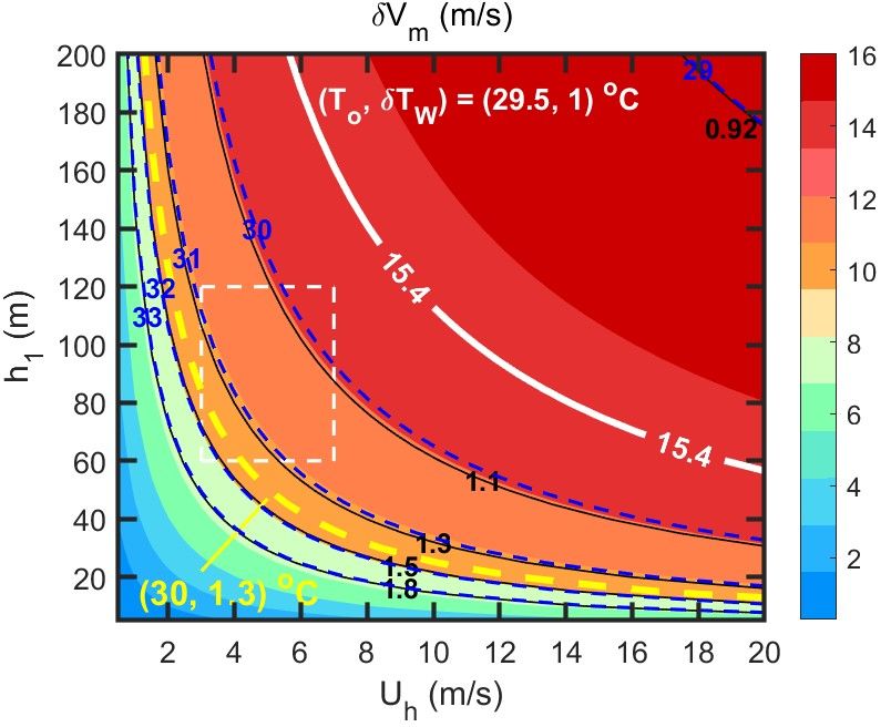
Atmosphere 2021, 12, 1285                                                                                                     4 of 15

                            expressing mass and heat conservations. The SST after mixing is:

                                                   Tmix = T1 + δT,                      δT = −[h2 /(h1 + h2 )] ∆T,               (5)

                            where ∆T = T1 − T2 (> 0) is the differenced temperature of the two original layers. The
                            corresponding differenced density ∆$ = $1 − $2 (< 0):

                                                                         ∆$/$0 = −α ∆T,                                          (6)

                            where $0 is the reference seawater density ≈ 1025 kg/m3 , and α = (∂$/∂T)/$0 is the thermal
                            expansion coefficient of seawater, ≈ 3×10⁻⁴ K−1 at the sea surface with SST ≈ 28 ◦ C and
                            salinity ≈35 psu.

                            2.3.3. Potential Energy
                                 Wind work raises the potential energy (PE) of the fluid by mixing it. Equating the
                            raised PE = PE|mix − PE|2layers to wind work yields a formula relating the wind to density
                            (and temperature). Thus, since
                                                                   Z 0                         Z −h
                                                                                                    1
                                                   PE2layers =                $1 g zdz0 +                 $2 g zdz0 ,            (7)
                                                                       − h1                     −h1 −h2

                            and                                                Z 0
                                                             PEmix =                         $mix g zdz0 ,                       (8)
                                                                                   −h1 −h2

                            we obtain
                                             PE = −(g/2) ∆$ h2 h1 = (g/2) α $0 ∆T h2 h1                            (J/m2 ).      (9)

                            2.3.4. Wind Energy
                                 The wind power on the ocean is $a Cd V3 in J/(m2 ·s), the scalar product of the surface
                            drag $a Cd |V|V and wind V, neglecting the ocean current. Here, $a is the air density, Cd
                            is the drag coefficient, and V = |V| the wind speed. Due to the TC’s size, the redpoint
                            (Figure 1) experiences the wind and SST cooling hours or days before the storm arrives,
                            depending on Uh . Oey et al. [37] observed this ahead-of-storm SST cooling in buoy
                            measurements in the Caribbean Sea before the arrival of Hurricane Wilma (2005). Therefore
                            the wind energy for mixing at the redpoint is:
                                                                              Z P                  
                                                           WE = γ                   $a Cd V3 dt J/m2 .                         (10)
                                                                               0

                                  Here, the mixing efficiency γ takes into account that only a fraction of the wind work
                            goes into mixing, and P = L/Uh , where L ≈ storm’s radius. The integral is from t = 0 when
                            the outer-most circle of weak TC wind influences the redpoint to t = P when the TC center
                            arrives (one could formally transform the integral by setting x = −Uh t + L + xredpoint but
                            thinking in “t” is more straightforward). We neglect the contribution from the generally
                            even weaker, non-TC wind before the TC’s outer-most circle arrives. We also assume that
                            after time t = P, SST cooling at the redpoint will not affect intensity. For t > P, the TC center
                            has passed the redpoint. Thus, ignoring the short distance across the back half of the eye,
                            ocean cooling in the TC’s wake has a minor further impact on intensity.

                            2.3.5. Wind-Induced SST Cooling
                                  Set PE = WE, and use (5) to yield:
                                                                   P
                                                        Z                       h            i h      
                                                                                    3g                   2
                                          Tmix   = T1 − γ              $a Cd V dt /     α$0 h2 h1              .               (11)
                                                               0                     2               h2 + h1
The Increased Likelihood in the 21st Century for a Tropical Cyclone to Rapidly Intensify When Crossing a Warm Ocean Feature-A Simple Model's ...
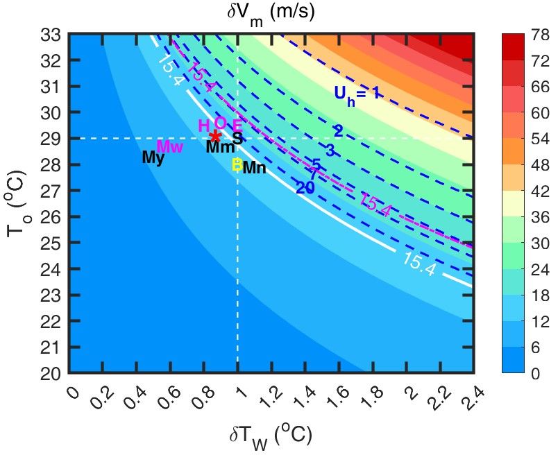
Atmosphere 2021, 12, 1285                                                                                              5 of 15

                            Piecewise continuous formulae of V are available [43] to evaluate the integral. To obtain
                            simple formulae, we choose to model V as a simple rise and fall as the TC passes the point:

                                                  V = V0 sin[πt/(2P)],           V0 = maximum wind,                     (12)

                            Thus, ignoring the rapid wind change with two maxima as the TC center passes. Because of
                            integration, the exact form is not crucial. Using Equation (12) in Equation (11), we obtain:
                                                                                h g 
                                                             4      L      $a        3
                                                                                                       i
                                           Tmix = T1 −                          γCd V0 /         α h h1 ,           (13)
                                                            3π     Uh      $0                 2

                            where h = h1 + h2 . Equation (13) gives the cooled SST the arriving TC sees at a point ahead
                            of the TC path, including the redpoint. The SST cooling (= Tmix − T1 ) is inversely related
                            to Uh and h1 . It shows that a slower storm sees a cooler SST than a faster one, and a thicker
                            upper warm layer is less susceptible to cooling than a thinner one.

                            2.3.6. Coupling
                                Focusing on the redpoint, as the TC crosses into the WOF, we assume that its maximum
                            wind V0 changes while its temporal functional form remains unchanged:

                                                                δV ≈ δV0 sin[πt/(2P)].                                  (14)

                            This is a good approximation since the redpoint is only a short distance into the WOF. We
                            can then use Equation (11) to relate the change in SST due to a change in the wind. Taking
                            δ of Equation (11) and evaluating the integral (or taking δ of Equation (13)):

                                                               δT0 = −δV0 FT                                            (15)
                                                                      
                                                          8   L     $a
                                                   FT =                 Cd V20 /[gα h h1 ].                             (16)
                                                          π   Uh    $0
                            The special notation δT0 (with subscript ‘o’) is used instead of δTmix , as a reminder that it is
                            the ocean cooling caused by increased δV0 as the TC crosses into the WOF. At the redpoint,
                            the total SST change is the sum of the warmer SST due to the WOF and cooling due to
                            ocean mixing:
                                                              δTredpoint = δTW + δT0 .                                 (17)
                                 The V0 refers to the incoming TC that translates into the WOF. To close the model (i.e.,
                            to couple), one needs to relate δV0 to δVm , where δVm depends on SST from Equation (3).
                            A reasonable assumption is that δV0 /δVm is proportional to V0 /Vm , and we set the propor-
                            tionality to one for simplicity. The assumption is equivalent to letting V0 be proportional to
                            Vm , such that their ratio is approximately invariant, as the data and analysis of [6,33–35]
                            suggest. Thus:
                                                             δV0 = µ δVm , µ = V0 /Vm ≤ 1.                           (18)
                            The µ is .0.5 for V0 . 50 m/s and tropical/subtropical SST & 28 ◦ C (Figure 2) (in Oey and
                            Huang [30], we set δV0 = δVm , i.e., µ =1, which overestimates the cooling, although their
                            conclusions remain unchanged).
                                Setting δT = δTredpoint and using Equations (15)–(18) in Equation (3) yields a quadratic
                            equation for δVm . Both roots are positive, but the smaller root is physically plausible:
                                                                         q
                                                         δVm = [µ2 −         µ22 − 4µ1 µ3 ]/[2µ1 ]                      (19)

                                                   µ1 = sC(µFT )2 /2, µ2 = 1 + (1 + CδTW )sµFT ,
                                                   µ3 = sδTW (1 + CδTW /2).
                            Taylor’s expansion in small FT shows that the solution tends to Equation (3) without ocean
                            cooling as FT ~ 0.
The Increased Likelihood in the 21st Century for a Tropical Cyclone to Rapidly Intensify When Crossing a Warm Ocean Feature-A Simple Model's ...
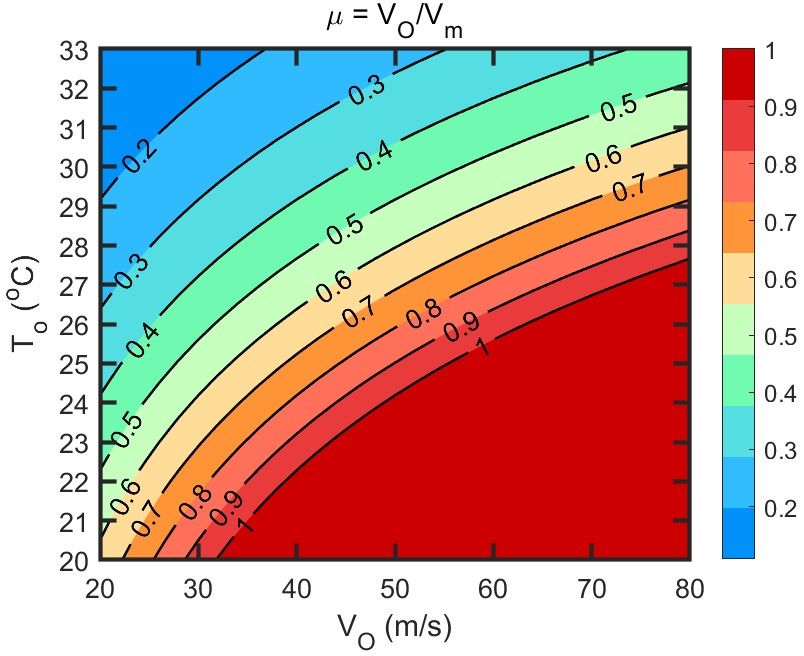
Atmosphere 2021, 12, 1285                                                                                                                   6 of 15
 Atmosphere 2021, 12, x FOR PEER REVIEW                                                                                                      6 of 15

                                  Figure2.2.Plot
                                 Figure      Plotof
                                                  ofµμ==VV0O/V
                                                            /Vmm..

                                       Although Equation (19) will be used in the plots, we can more easily see the effect of
                                 oceanSetting
                                         feedback                                  2 ) term in Equation (3). The solution is:
                                                   δTby   dropping
                                                       = δT redpoint andtheusing
                                                                            O(δTEquations        (15)–(18) in Equation (3) yields a quadrat‐
                                  ic equation for δVm. Both roots are positive, but the smaller root is physically plausible:
                                                                     δVm = s(T0 )δTW /[1 + s(T0 )µFT ],                                       (20)
                                                                      δV = [μ − μ − 4μ μ ]/[2μ ]                                                (19)
                                 where s(T0 ) is a reminder that it depends on the ambient SST T0 .
                                                                          μ = sC(μF ) /2 , μ = 1 + (1 + CδT )sμF ,
                                 2.3.7. Values of Parameters              μ = sδT (1 + CδT /2).
                                  Taylor's expansion in small FT shows that the solution tends to Equation (3) without
                                       We use the following values of the model parameters:
                                  ocean cooling as FT ~ 0.                                                              ◦ C−1 for western North
                                 A = 15.69    (2758) m/s,
                                        Although             B = 98.03
                                                      Equation            (74.03)
                                                                    (19) will  be m/s,
                                                                                   usedand      C =plots,
                                                                                            in the   0.1806we (0.1903)
                                                                                                                 can more    easily see the effect
                                 Pacific
                                  of ocean(North    Atlantic),
                                              feedback           from Zeng
                                                          by dropping       theet  al. [6]
                                                                                O(δT         (Xu et
                                                                                        2) term   in al. [35]), see
                                                                                                     Equation     (3).Equation (2); is:
                                                                                                                       The solution
                                 L = 200 km, the TC’s radial scale (roughly to ~18 m/s) [40];
                                 $a /$0 = 10−3 , the ratio of air δV         = s(T )´δT
                                                                       to seawater             /[1 + s(T )´μF ],
                                                                                        densities;                                              (20)
                                    = 0.02,s(T
                                 γwhere      see  below;
                                               o) is a reminder that it depends on the ambient SST To.
                                 Cd = 2 × 10⁻³ , the drag coefficient at high wind speeds [47];
                                 g2.3.7. m/s2 , the
                                    = 10 Values        Earth’s gravity;
                                                   of Parameters
                                            10−the
                                      3 × use
                                 α = We          4 K−1 , seawater’s thermal expansion coefficient [39];
                                                     following values of the model parameters:
                                 hA1 and   h2 (2758)
                                     = 15.69   are chosen
                                                        m/s, Bto=be    from
                                                                    98.03     the surface
                                                                           (74.03)   m/s, and  toCthe   26 ◦ C (0.1903)
                                                                                                    = 0.1806                    −zwestern
                                                                                                                isotherm°Cz−1=for  26 , and North
                                                                                                                                            from
                                                                                                                                               ◦
                                   = −z26(North
                                 zPacific            20 ◦ C isotherm
                                             to the Atlantic),            z =  − z    . The
                                                                   from Zeng et20al. [6] (Xu  h  ≈  h
                                                                                               1 et al.  ≈ 100   m  in the RI region
                                                                                                      2 [35]), see Equation (2);       (10~25    N)
                                 in
                                  L the  tropical
                                     = 200  km, the and   subtropical
                                                       TC’s   radial scalewestern
                                                                             (roughly North    Pacific
                                                                                          to ~18   m/s)(Figure
                                                                                                          [40]; 3).
                                  ρa/ρo = 10−3, the ratio of air to seawater densities;
                                  γ = 0.02, see below;
                                  Cd = 2´10−3, the drag coefficient at high wind speeds [47];
                                  g = 10 m/s2, the Earth’s gravity;
                                  α = 3´10−4 K−1, seawater’s thermal expansion coefficient [39];
The Increased Likelihood in the 21st Century for a Tropical Cyclone to Rapidly Intensify When Crossing a Warm Ocean Feature-A Simple Model's ...
Atmosphere 2021, 12, x FOR PEER REVIEW                                                                                                      7 of 15

Atmosphere 2021, 12, 1285
                                h1 and h2 are chosen to be from the surface to the 26 °C isotherm z = −Z26, and from    z=
                                                                                                                     7 of 15
                                −Z26 to the 20 °C isotherm z = −Z20. The h1  h2 ≈ 100 m in the RI region (10~25 N) in the
                                                                                                                 °

                                tropical and subtropical western North Pacific (Figure 3).
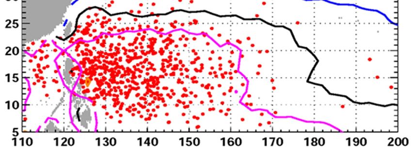
                                 Figure 3. Top:
                                           Top: mean
                                                 meanZ26
                                                       Z26(=(=hh1 )1)and
                                                                      andZ20-Z26
                                                                           Z20‐Z26(=(=h2h,2contours)
                                                                                           , contours)(m) from
                                                                                                        (m)     thethe
                                                                                                             from    EN4 reanalysis
                                                                                                                       EN4          [46].[46].
                                                                                                                            reanalysis     Bottom:
                                                                                                                                               Bot‐
                                tom:  RI locations
                                 RI locations as redasdots
                                                       red dots     [15] from
                                                            [15] from          IBTrACS
                                                                          IBTrACS           (https://www.ncdc.noaa.gov/ibtracs/
                                                                                     (https://www.ncdc.noaa.gov/ibtracs/             accessed
                                                                                                                                  accessed     onon
                                                                                                                                                  1
                                1October
                                   October  2021)
                                          2021)   and
                                                and    SST
                                                     SST     contours
                                                         contours      26,26,
                                                                           28,28,
                                                                              29, 29,  30 ◦30
                                                                                  andand        °C (blue,
                                                                                             C (blue,     black,
                                                                                                      black,     magenta,
                                                                                                             magenta,   and and orange).
                                                                                                                            orange).  OnlyOnly
                                                                                                                                             a fewa
                                few
                                 30◦ C30°C  contours
                                       contours       exist to
                                                exist close   close   to the Philippines’
                                                                the Philippines’               eastern
                                                                                    eastern coast.   Thecoast. The
                                                                                                          period     period is 1992–2015
                                                                                                                  is 1992–2015               June–
                                                                                                                               June–September.
                                September.
                                Choosing γ:
                                Choosing
                                      Givenγ: Z26 and Z20 as a slowly-varying background ocean state, one can calculate the
                                      Given ZδT(Z
                                SST cooling     26 and, Z20 ,as
                                                    26     20 Ua h ,slowly‐varying
                                                                     V0 ; γ) (Equationbackground
                                                                                          (13)) along aocean    state,
                                                                                                          storm’s      one
                                                                                                                   track     canγcalculate
                                                                                                                          with     serving asthe
                                                                                                                                               a
                                SST coolingHere
                                parameter.     δT(Zwe26, Zuse
                                                           20, U h, VEN4
                                                                the   O; γ) data
                                                                             (Equation
                                                                                  as the 13)   along
                                                                                           ocean       a storm's
                                                                                                   state  given astrack  with γ
                                                                                                                    monthly       servingfrom
                                                                                                                                analysis    as a
                                parameter.
                                1900          Here we
                                      to the present      useWe
                                                        [48].   thecalculate
                                                                     EN4 data   Uhasand
                                                                                      theVocean    state location
                                                                                            0 at a track  given asusing
                                                                                                                     monthly     analysisoffrom
                                                                                                                            the average      the
                                1900 to the
                                present   andpresent
                                               previous  [48].  Wevalues.
                                                            day’s     calculate
                                                                              WeU   h and
                                                                                  then      VO atγato
                                                                                         choose       track
                                                                                                        yieldlocation   usingthat
                                                                                                               SST cooling     the reasonably
                                                                                                                                    average of
                                the present
                                matches    theand   previous
                                                observed      andday's     values.
                                                                    full ocean      We then
                                                                                 model’s        choose
                                                                                             cooling   in γtwo
                                                                                                             to yield  SST cooling
                                                                                                                TCs: Typhoon          that
                                                                                                                                   Nuri     rea‐
                                                                                                                                         (2008)
                                sonably
                                and Typhoonmatches   the observed
                                                 Soudelor     (2015). We andpreviously
                                                                              full oceanconducted
                                                                                            model's cooling
                                                                                                        detailedinanalyses
                                                                                                                   two TCs:and Typhoon    Nuri
                                                                                                                                   SST cooling
                                simulations
                                (2008)        for these typhoons
                                        and Typhoon         Soudelorusing       theWe
                                                                          (2015).   Princeton
                                                                                        previouslyoceanconducted
                                                                                                         model (POM)       [16,49,50].
                                                                                                                     detailed          We find
                                                                                                                                 analyses   and
                                that γcooling
                                SST     = 0.02 gives   reasonably
                                                simulations       for good
                                                                       theseagreements
                                                                               typhoons usingbetween        and SST cooling
                                                                                                     theδTPrinceton             from GHRSST
                                                                                                                       ocean model      (POM)
                                observationWe
                                [16,49,50].    and  POM
                                                  find   that(Figure
                                                               γ = 0.024). gives
                                                                            The γreasonably
                                                                                   = 0.02 is within
                                                                                                 goodthe    range cited
                                                                                                         agreements       in the literature
                                                                                                                       between     δT and SSTfor
                                strong boundary
                                cooling   from GHRSSTstirring    at high buoyancy
                                                              observation     and POM   Reynolds
                                                                                            (Figurenumber
                                                                                                      4). The [51–54].
                                                                                                               γ = 0.02 is within the range
                                cited in the literature for strong boundary stirring at high buoyancy Reynolds number
                                [51–54].
Atmosphere 2021, 12, 1285                                                                                                                    8 of 15
here 2021, 12, x FOR PEER REVIEW                                                                                                       8 of 15

                             Figure 4. Comparisons
                 Figure 4. Comparisons                of theSST
                                          of the analytical  analytical
                                                                coolingSST  cooling
                                                                        (with        (with
                                                                               γ = 0.02)   γ =GHRSST
                                                                                         with  0.02) with GHRSST
                                                                                                        (Group      (Group
                                                                                                                for High    for HighSea Surface
                                                                                                                         resolution
                 Temperature, https://www.ghrsst.org/ accessed on 1 October 2021) and three-dimensional POM simulatedand
                             resolution Sea   Surface  Temperature,   https://www.ghrsst.org/    accessed  on 1  October  2021)   cooling along
                             three‐dimensional POM simulated cooling along the daily track of Typhoons Nuri [49,50] and
                 the daily track of Typhoons Nuri [49,50] and Soudelor [16]. Note that due to interpolation GHRSST tends to underestimate
                             Soudelor [16]. Note that due to interpolation GHRSST tends to underestimate TC‐induced SST
                 TC-induced SST cooling [49]. For Nuri, the discrepancy on Day 3 is due to the storm crossing the warm Kuroshio in the
                             cooling [49]. For Nuri, the discrepancy on Day 3 is due to the storm crossing the warm Kuroshio in
                 Luzon Strait,
                             thewhich
                                 Luzonthe  simple
                                        Strait,   model
                                                which thepoorly
                                                           simplerepresents.
                                                                  model poorly represents.

                              3. Results        3. Results
                                  We describe theWe  describeWOF‐induced
                                                  modeled     the modeled WOF-induced       intensity
                                                                             intensity change         change δV
                                                                                               δVm, focusing      m ,on
                                                                                                               first  focusing
                                                                                                                        the    first on the
                                           western   North  Pacific’s typhoons   since these have  the largest  intensity
                              western North Pacific's typhoons since these have the largest intensity changes. Then,      changes.    Then,
                                           however,   we will comment    on the North  Atlantic’s
                              however, we will comment on the North Atlantic's hurricanes.        hurricanes.

                                              3.1. δVm with No Ocean Feedback
                              3.1 δVm with no Ocean Feedback
                                                     Figure 5 (color shading) shows δVm without ocean feedback as a function of δTW
                                    Figure 5 (color shading) shows δVm without ocean                    feedback as a function of δTW
                                              and T0 . Mathematically, it is equivalent to the maximum possible increased intensity as
                              and To. Mathematically, it is equivalent to the maximum possible increased intensity as
                                              the storm enters the WOF at an infinite translation speed U . There is then little time for
                              the storm enters the WOF at an infinite translation speed Uh. There is thenh little time for
                                              ocean mixing by the wind to cool the sea surface. It is also the δVm when the TC crosses
                              ocean mixing by the wind to cool the sea surface. It is also the δVm when the TC crosses
                                              onto a shallow warm sea where the entire water column is well-mixed. The white line
                              onto a shallow warm sea where the entire water column is well‐mixed. The white line
                                              shows the corresponding δVm = 15.4 m/s separating the (δTW , T0 ) on the upper right
                              shows the corresponding δVm = 15.4 m/s separating the (δTW, To) on the upper right
                                              where a WOF-induced RI is possible from the lower-left where RI is unlikely. Figure 5 uses
                              where a WOF‐induced           RI is possible from the lower‐left where RI is unlikely. Figure 5
                                              V0 = 30 m/s as a representative example. Most observed RIs develop when the TC is in the
                              uses Vo = 30 m/s   as a representative
                                              tropical    storm (TS) or example.
                                                                            CategoriesMost      observed
                                                                                           1–2 stages        RIs develop when
                                                                                                        [15,17,18,30,36].    However,the TCtheisδVm = 15.4 m/s
                              in the tropical line
                                               storm    (TS)   or  Categories      1–2  stages  [15,17,18,30,36].     However,
                                                    in this plot and Figure 6, hence the inferences derived from it are independent the  δV  m =
                                                                                                                                                          of V0
                              15.4 m/s line in   this   plot  and    Figure     6, hence   the  inferences      derived   from   it  are
                                              since the line is for the asymptotic limit of zero ocean cooling. The present climatologicalinde‐
                              pendent of Vo since
                                              SST (T  the) in
                                                           line
                                                              theisRI
                                                                    forregion
                                                                        the asymptotic
                                                                                 is 28–29.5 limit   of zero
                                                                                             ◦ C (Figure    3).ocean  cooling. The
                                                                                                                The composite           present mean eddy’s
                                                                                                                                   (1993–2015)
                                                       0
                              climatological SST
                                              SST anomaly
                                                     (To) in theis +0.3 C [55], but δTW in individual WOFs can reach +1(1993–
                                                                     RI  region
                                                                          ◦        is 28–29.5   °C   (Figure    3). The   composite       ◦ C [15,16,24,27]. For
                              2015) mean eddy's     SST anomaly
                                              reference,               is +0.3 lines
                                                             white dashed        °C [55],  but δTthe
                                                                                       indicate    W in individual WOFs can reach +1
                                                                                                       present climate’s (δTW , T0 ) = (1, 29) ◦ C. As the
                              °C [15,16,24,27].majority
                                                 For reference,
                                                            (~85%)white
                                                                     of RIsdashed
                                                                               occur forlines
                                                                                           Uhindicate
                                                                                               . 7 m/sthe      present
                                                                                                           [6,36],       climate’s
                                                                                                                    the result       (δTW, that
                                                                                                                                suggests     To) RIs triggered
                              = (1, 29) °C. Asby
                                               thethe
                                                    majority     (~85%)     of  RIs  occur  for U h ≲  7  m/s   [6,36], the  result   suggests
                                                        WOF alone are unlikely to be frequent occurrences in the present climate. In other
                              that RIs triggered   by the
                                              words,          WOF
                                                         factors      alone
                                                                   other   thanareWOF
                                                                                    unlikely
                                                                                          alonetomore
                                                                                                  be frequent      occurrences
                                                                                                         likely trigger    the RIsinobserved
                                                                                                                                       the pre‐ in the present
                              sent climate. Inclimate.
                                                 other words,       factors
                                                           See Section 3.3.    other  than   WOF     alone   more    likely  trigger    the RIs
                              observed in the present climate. See section 3.3.

                              3.2 δVm with Ocean Feedback
                                   In Equation (20), the "s ´ δTW" is the MPI estimate of the WOF‐induced intensifica‐
                              tion. The "s ´ μFT" (> 0) is the coupling term that includes the contribution (FT) from
                              ocean cooling caused by the mixing of surface and subsurface water by the translating
                              storm. The formula shows that ocean cooling always reduces δVm. Since FT is inversely
                              related to Uh and h1 (see Equation 16), the ocean cools more for slower storms, a thinner
                              upper warm layer, or both, which then reduces δVm. For very deep h1, FT ~ 0, and ocean
                              feedback is negligible. Ocean feedback is also weak for very fast storms since there is lit‐
Atmosphere 2021, 12, x FOR PEER REVIEW                                                                                                       9 of 15

Atmosphere 2021, 12, 1285        tle time for the wind to mix the upper ocean, and the feedback to the storm is negligible.
                                                                                                                    9 of 15
                                 In either case, the intensification is due to the WOF alone and becomes the upper‐bound
                                 MPI estimate: δVm = s ´ δTW.

                                  Figure5.5. Color
                                 Figure       Color shading:
                                                     shading: western
                                                                western North
                                                                           North Pacific’s
                                                                                 Pacific’s δVδVmmfor
                                                                                                   forUUh ==
                                                                                                          h
                                                                                                            ∞∞(i.e., nono
                                                                                                                 (i.e.,  ocean feedback)
                                                                                                                           ocean          as TC
                                                                                                                                  feedback)       en‐
                                                                                                                                              as TC
                                  counters   a  WOF   with  δT W warmer than the ambient To; white line is δVm = 15.4 m/s. Blue dashed
                                 encounters a WOF with δTW warmer than the ambient T0 ; white line is δVm = 15.4 m/s. Blue
                                  lines are 15.4 m/s with ocean feedback for various Uh. White dashed lines mark To = 29 °C and δTW
                                 dashed lines are 15.4 m/s with ocean feedback for various Uh . White dashed lines mark T0 = 29 ◦ C
                                  = 1 °C. Letters are observed RI TCs: Bansi (2015; pre‐RI intensity (pRIi) Cat.2) [28], Earl (2010; pRIi
                                 and δTW = 1 ◦ C. Letters are observed RI TCs: Bansi (2015; pre-RI intensity (pRIi) Cat.2) [28], Earl
                                  Cat.1) [27], Harvey (2017; pRIi TS) [29], Maemi (2003; pRIi Cat.1) and Maon (2004; pRIi Cat.1) [24],
                                 (2010;
                                  ManyipRIi    Cat.1)
                                           (2013;     [27],
                                                   pRIi  TS)Harvey    (2017; pRIi
                                                              [12], Matthew       TS) [29],
                                                                                (2016;  pRIiMaemi
                                                                                               Cat.1) (2003;  pRIi Cat.1)
                                                                                                        [56], Opal    (1995;and
                                                                                                                             pRIiMaon  (2004;
                                                                                                                                   Cat.1)  [22],pRIi
                                                                                                                                                 and
                                 Cat.1)  [24],(2015;
                                  Soudelor     ManyipRIi
                                                       (2013;
                                                          TS)pRIi
                                                               [16].TS)
                                                                      The[12],
                                                                           red Matthew
                                                                               asterisk is(2016;
                                                                                            their pRIi
                                                                                                  mean. Cat.1)
                                                                                                           The [56],  Opal (1995;
                                                                                                               Uh ranges    from 3pRIi
                                                                                                                                    (Mn)Cat.1)
                                                                                                                                          to 8.5[22],
                                                                                                                                                 m/s
                                 and
                                  (O).Soudelor
                                       The magenta(2015;  pRIi
                                                       line     TS)
                                                            is δV m =[16].
                                                                       15.4The
                                                                            m/s red asterisk
                                                                                for the        is their(no
                                                                                        N Atlantic       mean.
                                                                                                            oceanThe    Uh ranges
                                                                                                                    feedback).  Thefrom
                                                                                                                                    model3 (Mn)
                                                                                                                                            uses γto=
                                 8.5 m/s
                                  0.02, h1 (O).
                                           = h2 The
                                                = 100magenta
                                                       m and Vline   is δV
                                                                 O = 30    m = 15.4 m/s for the N Atlantic (no ocean feedback). The model
                                                                        m/s.
                                 uses γ = 0.02, h1 = h2 = 100 m and V0 = 30 m/s.
                                         The blue dashed lines in Figure 5 show the δVm = 15.4 m/s contours obtained from
                                 3.2.
                                  the δV  m with Ocean
                                        solution         Feedback
                                                  with ocean    feedback for different Uh. (The plot is for the solution 19, alt‐
                                        In Equation  (20), the “s
                                  hough the quadratic correction   × δTWis” small:
                                                                            is the MPI estimate
                                                                                   5–10%         of the WOF-induced
                                                                                           less cooling).              intensification.
                                                                                                           Ocean cooling    at finite Uh
                                 The   “s  ×  µF
                                  shifts the 15.4 ” (> 0) is the  coupling   term  that includes  the  contribution
                                                 T m/s line rightward and upward, meaning ocean feedback Tmakes      (F  ) from it
                                                                                                                                 ocean
                                                                                                                                    even
                                 cooling    caused  by the mixing   of surface   and subsurface
                                  harder for WOF‐induced RI to develop under the present climate.water  by the translating  storm.  The
                                 formula shows that ocean cooling always reduces δVm . Since FT is inversely related to Uh
                                 and
                                  3.3. hObserved
                                         1 (see Equation   (16)),
                                                  RIs in the      the ocean
                                                             Present  Climatecools more for slower storms, a thinner upper warm
                                 layer, or both, which then reduces δVm . For very deep h1 , FT ~ 0, and ocean feedback is
                                         Figure 5 plots the (δTW, To) points of nine TCs whose RIs may be related to WOFs
                                 negligible. Ocean feedback is also weak for very fast storms since there is little time for the
                                  (source references in the caption). We only include Tropical Cyclone Bansi for compari‐
                                 wind to mix the upper ocean, and the feedback to the storm is negligible. In either case,
                                  son since the empirical MPI used is not for the South Indian Ocean. The magenta line
                                 the intensification is due to the WOF alone and becomes the upper-bound MPI estimate:
                                  shows the 15.4 m/s using Xu et al.'s [35] empirical MPI coefficients for the North Atlan‐
                                 δVm = s × δTW .
                                  tic. We use it to assess the four Atlantic hurricanes (E, H, Mw, and O). The magenta line
                                        The blue dashed lines in Figure 5 show the δVm = 15.4 m/s contours obtained from
                                  shifts slightly rightward and upward relative to the western North Pacific line (white)
                                 the solution with ocean feedback for different Uh . (The plot is for the solution 19, although
                                  because the Atlantic's slope ∂Vm/∂T is less steep (roughly 0.8:1). The 9‐TCs' mean (δTW,
                                 the quadratic correction is small: 5–10% less cooling). Ocean cooling at finite Uh shifts the
                                  To) are (0.87, 28.8) °C (red asterisk), and the mean Uh is 5.2 m/s. The plot shows that none
                                 15.4 m/s line rightward and upward, meaning ocean feedback makes it even harder for
                                  of the TCs' rapid intensifications was WOF‐induced. Typhoon Soudelor is the only
                                 WOF-induced RI to develop under the present climate.
Thus, δVm is ~5 times more sensitive to δTW than To (the sensitivity difference is some‐
                             what reduced by ocean feedback (the O(sμFT) term) especially when h1 or Uh or both are
                             small). Thus a 1 °C change in To takes only ~0.2 °C change in δTW to effect the same in‐
                             tensity change. For example, Figure 6 shows that a 0.3 °C (0.5 °C) change of δTW from 1
Atmosphere 2021, 12, 1285    to 1.3 °C (1.5 °C) increases the likelihood for WOF‐induced RIs as the region where
                                                                                                               10 ofδV
                                                                                                                     15m
                             > 15.4 m/s sweeps across more than 60% (95%) of the box. The effect is the same as a 1.5
                             °C (2.5 °C) change in To from 29.5 to 31 (32) °C.

                             Figure6.6.Western
                            Figure      WesternNorth
                                                  NorthPacific’s
                                                          Pacific’sδVδV
                                                                      mmasasa afunction
                                                                                 function ofof
                                                                                             UhUand
                                                                                                 h and
                                                                                                     h1hfor
                                                                                                         1 for
                                                                                                             (T(T    , δT
                                                                                                                0 , oδT WW      (29.5,1)1)◦ C
                                                                                                                          ) )==(29.5,       oC (shading
                                                                                                                                              (shading
                             and white    15.4 m/s‐line).  Other  lines  are  15.4   m/s  for blue  dashed:   T o = 29, 30, 31, 32, 33◦ oC at fixed
                            and white 15.4 m/s-line). Other lines are 15.4 m/s for blue dashed: T0 = 29, 30, 31, 32, 33 C at fixed
                             δTW== 11◦oC;
                            δT         C; black:
                                           black:δT
                                                  δTW == 0.92,
                                                         0.92, 1.1,
                                                               1.1,1.3,
                                                                    1.3,1.5,
                                                                         1.5,1.8
                                                                               1.8◦ C
                                                                                    oC at fixed To = 29.5 oC; yellow: (To, δTW) = (30, 1.3) oC.
                                                                                      at fixed T0 = 29.5 ◦ C; yellow: (T0 , δTW ) = (30, 1.3) ◦ C.
                               W                    W
                             The white dashed box shows the 3 ≤ Uh ≤ 7 m/s and 60 ≤ h1 ≤ 120 m region where RI events are fre‐
                            The white dashed box shows the 3 ≤ Uh ≤ 7 m/s and 60 ≤ h1 ≤ 120om region where RI events are
                             quently observed. The model uses γ = 0.02 and VO = 30 m/s. Add 3 C ◦to To to apply the plot to the
                            frequently observed. The model        uses γ = 0.02 and V = 30 m/s. Add 3 C to T to apply the plot to
                             Atlantic hurricanes, i.e., 29.5 oC becomes 32.5 oC, 300oC becomes 33 oC, etc. 0
                            the Atlantic hurricanes, i.e., 29.5 ◦ C becomes 32.5 ◦ C, 30 ◦ C becomes 33 ◦ C, etc.
                                   One may
                            3.3. Observed   RIsquestion  the suitability
                                                in the Present Climate of using the empirical MPI relationship (Equation
                             2.2) based on present climate's data to make future inferences. In the absence of data, it
                                  Figure 5 plots the (δT , T0 ) points of nine TCs whose RIs may be related to WOFs
                             is, of course, impossible toWaddress     this with absolute certainty. However, we can make
                            (source references in the caption). We only include Tropical Cyclone Bansi for comparison
                             some reasonable deductions that the empirical relation will remain valid, at least into the
                            since the empirical MPI used is not for the South Indian Ocean. The magenta line shows
                             21st century. First, the theoretical MPI critically depends on the saturation mixing ratio,
                            the 15.4 m/s using Xu et al.’s [35] empirical MPI coefficients for the North Atlantic. We
                             which varies exponentially with SST according to the Clausius–Clapeyron relationship
                            use it to assess the four Atlantic hurricanes (E, H, Mw, and O). The magenta line shifts
                             [63,64]. Thus, the exponential form of the empirical MPI relationship is likely to remain
                            slightly rightward and upward relative to the western North Pacific line (white) because
                             valid
                            the      in the future.
                                 Atlantic’s  slope ∂VSecond,   any numerical change in the empirical MPI is likely to be
                                                       m /∂T is less steep (roughly 0.8:1). The 9-TCs’ mean (δTW , T0 ) are
                             'slow'.28.8)
                            (0.87,    Evidence   of asterisk),
                                          ◦ C (red  the slow change
                                                               and theismean
                                                                         that the exponent
                                                                               Uh is 5.2 m/s.coefficient
                                                                                               The plot C   remains
                                                                                                          shows thatstable
                                                                                                                     none de‐
                                                                                                                           of
                            the TCs’ rapid intensifications was WOF-induced. Typhoon Soudelor is the only stormC
                             spite  the  different periods  and  regions  in the four cited studies. In  the North Atlantic,
                            that crosses the white 15.4 m/s-line. However, ocean cooling at Uh = 5.5 m/s would also
                            render a WOF-induced RI unlikely in Soudelor. Instead, Oey and Lin [16] argued that
                            weakened environmental vertical wind shear < 4 m/s contributes to the storm’s RI [5].
                            They also suggested that weak vertical wind shears may have contributed to the RIs in
                            Hurricane Opal [57] and Typhoon Maemi [16]. These results show that for WOF-induced
                            RIs to develop, the WOF and ambient SST would have to be warmer than the present-day
                            T0 ≈ 28–29.5 ◦ C and δTW . 1 ◦ C. Thus, as stated before, RIs triggered by the WOF alone
                            are unlikely to be frequent occurrences in the present climate. Oey and Huang [30] arrived
                            at this same conclusion in numerical experiments designed to isolate the WOF-induced
                            intensity change. They found that although WOF increases intensity, the intensification
                            is insufficient to trigger more RIs. Consequently, the number of RIs is not statistically
Atmosphere 2021, 12, 1285                                                                                          11 of 15

                            significantly different between ensemble simulations with and without the WOF included
                            in the model.

                            4. Discussion
                                  Three of the four listed typhoons in Figure 5 are close to the white 15.4 m/s-line.
                            Thus, they are close to a “tipping point or line”, meaning that slight increases in T0 or
                            δTW or both may potentially foster more RIs. We use the simple model to project how
                            WOF-induced RIs may evolve as the Earth’s climate warms. The SST trend is +0.1 ◦ C
                            per decade in the western North Pacific, but two times higher in the Philippines Sea
                                             ◦
                            (latitudes . 20 N) [58–60]. Similar warming trends occur in the Atlantic. At these rates
                            and assuming that SST continues to rise [61], T0 would reach 30–31 ◦ C near the end of the
                            21st century.
                                  SSTs in coastal seas and western boundary currents show higher rates of warming
                            trends [60,62]. Along the western North Pacific rim and US southern and eastern shelves,
                            coastal SST trends reach +0.4 ◦ C per decade in summer [62], approximately two times
                            higher than the adjacent open seas. The value is consistent with a recent estimate of |∇SST|
                            trends of more than +0.2 ◦ C/100 km/decade) across China’s and Japan’s coastal shelves,
                            the northern Gulf of Mexico, the US south-mid-Atlantic, as well as across the Kuroshio and
                            the Gulf Stream [60]. At these rates, the corresponding δTW |Coast and δTW |WBC would
                            reach 1.2–1.8 ◦ C or more near the end of the 21st century. The trend of δTW |Eddy for
                            mesoscale eddies is harder to estimate. In the western North Pacific, Martínez-Moreno
                            et al. [60] show an increasing |∇SST| trend of +0.02 ◦ C/(100 km/decade) for eddies north
                            of 20 ◦ N, but a decreasing trend of −0.04 ◦ C/(100 km/decade) south of 20 ◦ N. The trends
                            in tropical and subtropical North Atlantic are similarly weakly decreasing. However, these
                            values for δTW |Eddy are weaker with larger uncertainty than the trends of δTW |Coast or
                            δTW |WBC .
                                  Figure 6 (color shading) shows δVm as a function of Uh and h1 for T0 = 29.5 ◦ C and
                            δTW = 1 ◦ C near their upper limits in the western North Pacific in the present climate. The
                            white line shows the corresponding δVm = 15.4 m/s separating the (Uh , h1 ) space on the
                            upper right where a WOF-induced RI is possible from the lower-left where RI is unlikely.
                            Ocean cooling is inversely related to h1 or Uh (Equations (15) and (16)). There is more (less)
                            cooling as the upper layer gets thinner (thicker), or the storm translates slower (faster), or
                            both. As a result, the atmospheric response is a weaker (stronger) δVm (Equation (3)). The
                            white dashed box encloses the RI region’s Z26 range (60–120 m; Figure 3) and the Uh range
                            (3–7 m/s; [36]), where the majority of RI events occur. Thus, as discussed before, one sees
                            that WOF-induced RIs in the present climate T0 . 29.5 ◦ C and δTW = 1 ◦ C are unlikely.
                                  Blue dashed lines show the sensitivity of intensity change to ambient SST at a fixed
                            δTW = 1 ◦ C. These 15.4 m/s lines shift left and down as the T0 increases, sweeping across the
                            white dashed box. For example, for a future T0 = 30 ◦ C, WOF-induced RIs can occur over
                            the small northeast corner of the box Uh > 5.5 m/s and Z26 > 95 m. When T0 = 31 (32) ◦ C,
                            the likelihood for WOF-induced RIs substantially increases as the region where δVm > 15.4
                            m/s now occupies 60% (95%) of the box.
                                  Black lines show the sensitivity of intensity change to WOF’s anomaly at a fixed
                            T0 = 29.5 ◦ C. Note that the dependency of δVm on h1 or Uh is unchanged, and one can
                            always find T0 and δT  W pair
                                                          for
                                                             which
                                                                   the blue dashed and black lines coincide. However,
                            from Equation (20), ∂δV      m
                                                     ∂δTW /
                                                               ∂δVm
                                                                ∂T0    ≈ 1/(δTW C) + 0(sµFT ), where C ≈ 0.18 ◦ C−1 (see
                            Section 2.2). Thus, δVm is ~5 times more sensitive to δTW than T0 (the sensitivity difference
                            is somewhat reduced by ocean feedback (the O(sµFT ) term) especially when h1 or Uh or
                            both are small). Thus a 1 ◦ C change in T0 takes only ~0.2 ◦ C change in δTW to effect the
                            same intensity change. For example, Figure 6 shows that a 0.3 ◦ C (0.5 ◦ C) change of δTW
                            from 1 to 1.3 ◦ C (1.5 ◦ C) increases the likelihood for WOF-induced RIs as the region where
                            δVm > 15.4 m/s sweeps across more than 60% (95%) of the box. The effect is the same as a
                            1.5 ◦ C (2.5 ◦ C) change in T0 from 29.5 to 31 (32) ◦ C.
Atmosphere 2021, 12, 1285                                                                                              12 of 15

                                  One may question the suitability of using the empirical MPI relationship (Equation (2))
                            based on present climate’s data to make future inferences. In the absence of data, it is, of
                            course, impossible to address this with absolute certainty. However, we can make some
                            reasonable deductions that the empirical relation will remain valid, at least into the 21st
                            century. First, the theoretical MPI critically depends on the saturation mixing ratio, which
                            varies exponentially with SST according to the Clausius–Clapeyron relationship [63,64].
                            Thus, the exponential form of the empirical MPI relationship is likely to remain valid in the
                            future. Second, any numerical change in the empirical MPI is likely to be ‘slow’. Evidence
                            of the slow change is that the exponent coefficient C remains stable despite the different
                            periods and regions in the four cited studies. In the North Atlantic, C = 0.1813, 0.1813,
                            and 0.1903 for the data from 1962–1992, 1981–2003, and 1988–2014, respectively [33–35],
                            while C = 0.1806 for the 1981–2003 data for the western North Pacific [6]. Zeng et al. [34]
                            made a similar argument when noting that the C they obtained was identical to DeMaria
                            and Kaplan’s [33] using an earlier dataset. Finally, in the simple model, the most critical
                            parameter is the slope s on the T-space. Based on the three analysis periods for the
                            North Atlantic hurricanes [33–35], s appears to be increasing. The s = 10.12, 11.71, and
                            14.09 m/s ◦ C−1 for the 1962–1992, 1981–2003, and 1988–2014 data. We do not know the
                            statistical significance of this increase. However, as long as this parameter is non-decreasing
                            with time, the model would not overpredict WOF-induced RIs.
                                  Rapid intensifications may become more frequent and storms more powerful as the
                            planet warms [65]. Our simple model also predicts this as the likelihood for RI increases
                            with increased ambient SST. Moreover, the greater sensitivity of RI to WOF anomaly
                            suggests more powerful landfalling TCs as storms cross warmer coastal seas and western
                            boundary currents. The simple model indicates that Western North Pacific coastlines:
                            China and Japan, are particularly vulnerable. Wada [12] already suggests such a possibility
                            with Typhoon Manyi crossing the warm Kuroshio south of Japan.

                            5. Conclusions
                                  This study presents a simple analytical model with ocean feedback of tropical cyclones’
                            rapid intensity change induced by warm ocean features (WOF). The model indicates that
                            WOF-induced rapid intensification (RI) is unlikely in the present climate. We provide
                            evidence of this inference using observations from nine TCs that developed RIs. We show
                            that the observed RIs have parameters below the model’s RI threshold. In other words, in
                            the present climate, other environmental and internal dynamical factors likely contributed
                            to the RIs observed in these TCs. The inference is in excellent agreement with the conclusion
                            of a recent numerical study [30].
                                  On the other hand, the simple model shows that WOF-induced RI is very sensitive
                            to the WOF’s anomalous amplitude, five times more sensitive than the background SST.
                            Thus, as coastal seas and western boundary currents continue to warm in the 21st century,
                            the model suggests an increased likelihood for RIs near the coasts, China and Japan
                            in particular. Future work may seek to show evidence of this prediction by analyzing
                            landfalling TCs. This model prediction that WOF-induced RI by increased δTW |Coast or
                            δTW |WBC

                            Funding: This research received no external funding.
                            Institutional Review Board Statement: Not applicable.
                            Informed Consent Statement: Not applicable.
                            Data Availability Statement: The observational data presented in this study are available from the
                            cited public links and references, IBTrACS (https://www.ncdc.noaa.gov/ibtracs/ accessed on 1
                            October 2021), and GHRSST (https://www.ghrsst.org/ accessed on 1 October 2021).
                            Acknowledgments: I thank the three reviewers for their inputs.
Atmosphere 2021, 12, 1285                                                                                                           13 of 15

                                  Conflicts of Interest: The author declares no conflict of interest. The funders had no role in the design
                                  of the study; in the collection, analyses, or interpretation of data; in the writing of the manuscript, or
                                  in the decision to publish the results.

                                  Appendix A. Symbols and Abbreviations
                                    A, B, C          Coefficients of the empirical MPI
                                    c                Ocean’s mode-1 baroclinic phase speed
                                    Cd               Drag coefficient
                                    FT               Factor expressing the effect of TC-induced SST cooling (Equation (16)); the term
                                                     “sµFT ” couples TC’s δVm to ocean cooling
                                    g                Earth’s gravity
                                    h 1 & h2         Depths of the ocean’s upper and lower layers, i.e. before mixing
                                    L                TC’s radius
                                    P                = L/Uh , time taken for the TC to traverse its radius (i.e. half its size)
                                    PE               Raised potential energy, PE after mixing minus before mixing
                                    PE|2layers       Ocean 2-layer system’s potential energy before mixing
                                    PE|mix           Ocean 1-layer system’s potential energy after mixing
                                    s                slope of Vm on the T-space: (∂Vm /∂T)|0
                                    t                a general variable for time
                                    T                a general variable for SST
                                    T1 and T2        Uniform temperatures of the ocean’s upper and lower layers before mixing
                                    Tmix             Uniform temperature after mixing
                                    T0               Ambient (i.e. background) SST (Figure 1)
                                    Uh               TC translation speed
                                    V                = |V| wind speed of the wind vector V
                                    Vm               MPI maximum wind
                                    V0               Maximum wind of the TC approaching the WOF
                                    WE               Wind energy
                                    x&z              Horizontal and vertical axes, z = 0 at the sea surface
                                    Z26 & Z20        Depths of the ocean’s 26 ◦ C and 20 ◦ C isotherms
                                    α                thermal expansion coefficient of seawater ≈ 3×10⁻⁴ K−1 at SST ≈ 28 ◦ C
                                    $a               Air density
                                    $0               Reference seawater density ≈ 1025 kg/m3
                                    $1 and $2        Uniform densities of ocean’s upper and lower layers before mixing
                                    $mix             Uniform seawater density after mixing
                                    δT               = Tmix − T1 (< 0), the SST cooling due to TC (Equation (13)); used also as the
                                                     usual mathematical notation of “Change in T” (e.g. Equation (3))
                                    δT0              < 0, ocean cooling caused by increased δV0 as the TC crosses into the WOF
                                    δTW              The WOF’s SST anomaly (> 0); i.e. total WOF’s SST = T0 + δTW (Figure 1)
                                    ∆T               = T1 − T2 (> 0), the temperature difference between upper and lower layers
                                    ∆$               = $1 − $2 (< 0), the density difference between upper and lower layers
                                    δVm              Change in MPI maximum wind (m/s) due to change in SST, see Equation (2)
                                    δV0              Change in TC’s maximum wind as it crosses over the WOF
                                    γ                Mixing efficiency (~ fraction of the wind work that goes into mixing)
                                    µ                Ratio of TC wind to MPI wind = V0 /Vm ≤ 1
                                    µ1 , µ2 , µ3     Coefficient variables used in the model solution (19)
                                    MPI              Maximum Potential Intensity
                                    POM              Princeton Ocean Model
                                    RI               Rapid Intensification
                                    SST              Sea Surface Temperature
                                    TC               Tropical Cyclone
                                    TS               Tropical Storm
                                    WOF              Warm Ocean Feature

References
1.    Kaplan, J.; DeMaria, M. Large-scale characteristics of rapidly intensifying tropical cyclones in the North Atlantic basin. Weather
      Forecast. 2003, 18, 1093–1108. [CrossRef]
Atmosphere 2021, 12, 1285                                                                                                            14 of 15

2.    Montgomery, M.T.; Nguyen, S.V.; Smith, R.K.; Persing, J. Do tropical cyclones intensify by WISHE? Q. J. R. Meteorol. Soc. 2009,
      135, 1697–1714. [CrossRef]
3.    Doyle, J.D.; Moskaitis, J.R.; Feldmeier, J.W.; Ferek, R.J.; Beaubien, M.; Bell, M.M.; Cecil, D.L.; Creasey, R.L.; Duran, P.; Elsberry,
      R.L.; et al. A view of tropical cyclones from above. BAMS 2017, 2113–2134. [CrossRef]
4.    Chen, X.; Zhang, J.A.; Marks, F.D. A thermodynamic pathway leading to rapid intensification of tropical cyclones in shear.
      Geophys. Res. Lett. 2019, 46, 9241–9251. [CrossRef]
5.    Paterson, L.A.; Hanstrum, B.N.; Davidson, N.E.; Weber, H.C. Influence of Environmental Vertical Wind Shear on the Intensity of
      Hurricane-Strength Tropical Cyclones in the Australian Region. Mon. Weather Rev. 2005, 133, 3644–3660. [CrossRef]
6.    Zeng, Z.; Wang, Y.; Wu, C.C. Environmental dynamical control of tropical cyclone intensity—An observational study. Mon. Wea.
      Rev. 2007, 135, 38–59. [CrossRef]
7.    Kaplan, J.; DeMaria, M.; Knaff, J.A. A revised tropical cyclone rapid intensification index for the Atlantic and eastern North
      Pacific basins. Weather Forecast. 2010, 25, 220–241. [CrossRef]
8.    Hendricks, E.A.; Peng, M.S.; Fu, B.; Li, T. Quantifying environmental control on tropical cyclone intensity change. Mon. Weather
      Rev. 2010, 138, 3243–3271. [CrossRef]
9.    Wu, L.; Su, H.; Fovell, R.G.; Wang, B.; Shen, J.T.; Kahn, B.H.; Hristova-Veleva, S.M.; Lambrigtsen, B.H.; Fetzer, E.J.; Jiang, J.H.
      Relationship of environmental relative humidity with North Atlantic tropical cyclone intensity and intensification rate. Geophys.
      Res. Lett. 2012, 39, L20809. [CrossRef]
10.   Soloviev, A.V.; Lukas, R.; Donelan, M.A.; Haus, B.K.; Ginis, I. The air-sea interface and surface stress under tropical cyclones. Sci.
      Rep. 2014, 4, 5306. [CrossRef]
11.   Soloviev, A.V.; Lukas, R.; Donelan, M.A.; Haus, B.K.; Ginis, I. Is the state of the air-sea interface a factor in rapid intensification
      and rapid decline of tropical cyclones? J. Geophys. Res. Oceans. 2017, 122, 10–174. [CrossRef]
12.   Wada, A. Unusually rapid intensification of Typhoon Man-yi in 2013 under preexisting warm-water conditions near the Kuroshio
      front south of Japan. J. Oceanogr. 2015, 71, 131–156. [CrossRef]
13.   Donelan, M.A. On the decrease of the oceanic drag coefficient in high winds. J. Geophys. Res. Oceans 2017, 123, 1485–1501.
      [CrossRef]
14.   Chen, X.; Wang, Y.; Zhao, K. Synoptic flow patterns and large-scale characteristics associated with rapidly intensifying tropical
      cyclones in the South China Sea. Mon. Weather Rev. 2015, 143, 64–87. [CrossRef]
15.   Zhang, L.; Oey, L. Young ocean waves favor the rapid intensification of tropical cyclones-a global observational analysis. Mon.
      Weather Rev. 2019, 147, 311–328. [CrossRef]
16.   Oey, L.; Lin, Y. The Influence of Environments on the Intensity Change of Typhoon Soudelor. Atmosphere 2021, 12, 162. [CrossRef]
17.   Kossin, J.P.; Olander, T.L.; Knapp, K.R. Trend analysis with a new global record of tropical cyclone intensity. J. Clim. 2013, 26,
      9960–9976. [CrossRef]
18.   Lee, C.-Y.; Tippett, M.K.; Sobel, A.H.; Camargo, S.J. Rapid intensification and the bimodal distribution of tropical cyclone intensity.
      Nat. Commun. 2016, 7, 10625. [CrossRef] [PubMed]
19.   Emanuel, K.A. Thermodynamic control of hurricane intensity. Nature 1999, 401, 665–669. [CrossRef]
20.   Schade, L.R.; Emanuel, K.A. The ocean’s effect on the intensity of tropical cyclones: Results from a simple coupled atmosphere–
      ocean model. J. Atmos. Sci. 1999, 56, 642–651. [CrossRef]
21.   Emanuel, K.; DesAutels, C.; Holloway, C.; Korty, R. Environmental control of tropical cyclone intensity. J. Atmos. Sci. 2004, 61,
      843–858. [CrossRef]
22.   Shay, L.K.; Goni, G.J.; Black, P.G. Effects of a warm oceanic feature on Hurricane Opal. Mon. Weather Rev. 2000, 128, 1366–1383.
      [CrossRef]
23.   Hong, X.; Chang, S.W.; Raman, S.; Shay, L.K.; Hodur, R. The interaction between Hurricane Opal (1995) and a warm core ring in
      the Gulf of Mexico. Mon. Wea. Rev. 2000, 128, 1347–1365. [CrossRef]
24.   Lin, I.I.; Wu, C.C.; Emanuel, K.; Lee, I.H.; Wu, C.R.; Pun, I.F. The interaction of Supertyphoon Maemi (2003) with a warm ocean
      eddy. Mon. Weather Rev. 2005, 133, 2635–2649. [CrossRef]
25.   Ali, M.M.; Jagadeesh, P.V.; Jain, S. Effects of eddies on Bay of Bengal cyclone intensity. Eos Trans. Am. Geophys. Union 2007, 88,
      93–95. [CrossRef]
26.   Mainelli, M.; DeMaria, M.; Shay, L.K.; Goni, G. Application of oceanic heat content estimation to operational forecasting of recent
      Atlantic category 5 hurricanes. Weather Forecast. 2008, 23, 3–16. [CrossRef]
27.   Jaimes, B.; Shay, L.K.; Uhlhorn, E.W. Enthalpy and momentum fluxes during Hurricane Earl relative to underlying ocean features.
      Mon. Weather Rev. 2015, 143, 111–131. [CrossRef]
28.   Mawren, D.; Reason, C.J.C. Variability of upper-ocean characteristics and tropical cyclones in the South West Indian Ocean. J.
      Geophys. Res. Oceans 2017, 122, 2012–2028. [CrossRef]
29.   Potter, H.; DiMarco, S.F.; Knap, A.H. Tropical Cyclone Heat Potential and the Rapid Intensification of Hurricane Harvey in the
      Texas Bight. J. Geophys. Res. Oceans. 2019, 124, 2440–2451. [CrossRef]
30.   Oey, L.; Huang, S.M. Can a warm ocean feature caus a typhoon to intensify rapidly? Atmosphere 2021, 12, 797. [CrossRef]
31.   Riehl, H. Some relations between wind and thermal structure of steady state hurricanes. J. Atmos. Sci. 1963, 20, 276–287.
      [CrossRef]
32.   Gray, W.M. Global view of the origin of tropical disturbances and storms. Mon. Wea. Rev. 1968, 96, 669–700. [CrossRef]
Atmosphere 2021, 12, 1285                                                                                                              15 of 15

33.   DeMaria, M.; Kaplan, J. Sea surface temperature and the maximum intensity of Atlantic tropical cyclones. J. Clim. 1994, 7,
      1325–1334. [CrossRef]
34.   Zeng, Z.; Chen, L.; Wang, Y. An observational study of environmental dynamical control of tropical cyclone intensity in the
      Atlantic. Mon. Weather Rev. 2008, 136, 3307–3322. [CrossRef]
35.   Xu, J.; Wang, Y.; Tan, Z. The relationship between sea surface temperature and maximum intensification rate of tropical cyclones
      in the North Atlantic. J. Atmos. Sci. 2016, 73, 4979–4988. [CrossRef]
36.   Zhang, L.; Oey, L. An observational analysis of ocean surface waves in tropical cyclones in the western North Pacific Ocean. J.
      Geophys. Res. Oceans 2019, 124, 184–195. [CrossRef]
37.   Oey, L.Y.; Ezer, T.; Wang, D.P.; Fan, S.J.; Yin, X.Q. Loop current warming by Hurricane Wilma. Geophys. Res. Lett. 2006, 33, L08613.
      [CrossRef]
38.   Oey, L.Y.; Ezer, T.; Wang, D.P.; Yin, X.Q.; Fan, S.J. Hurricane-induced motions and interaction with ocean currents. Cont. Shelf Res.
      2007, 27, 1249–1263. [CrossRef]
39.   Price, J.F. Upper Ocean Response to a Hurricane. J. Phys. Oceanogr. 1981, 11, 153–175. [CrossRef]
40.   Chelton, D.B.; de Szoeke, R.A.; Schlax, M.G.; El Naggar, K.; Siwertz, N. Geographical variability of the first-baroclinic Rossby
      radius of deformation. J. Phys. Oceanogr. 1998, 28, 433–460. [CrossRef]
41.   Xu, F.H.; Oey, L.Y. Seasonal SSH variability of the Northern South China Sea. J. Phys. Oceanogr. 2015, 45, 1595–1609. [CrossRef]
42.   Gill, A.E. Atmosphere-Ocean Dynamics; Academic Press: Cambridge, MA, USA, 1982; p. 662.
43.   Holland, G.J.; Belanger, J.I.; Fritz, A. A revised model for radial profiles of hurricane winds. Mon. Weather Rev. 2010, 138,
      4393–4401. [CrossRef]
44.   Chiang, T.L.; Wu, C.R.; Oey, L.Y. Typhoon Kai-Tak: A perfect ocean’s storm. J. Phys. Oceanogr. 2011, 41, 221–233. [CrossRef]
45.   Kunze, E. Near-inertial wave propagation in geostrophic shear. J. Phys. Oceanogr. 1985, 15, 544–565. [CrossRef]
46.   Oey, L.Y.; Inoue, M.; Lai, R.; Lin, X.H.; Welsh, S.E.; Rouse, L.J., Jr. Stalling of near-inertial waves in a cyclone. Geophys. Res. Lett.
      2008, 35, L12604. [CrossRef]
47.   Powell, M.D.; Vickery, P.J.; Reinhold, T.A. Reduced drag coefficient for high wind speeds in tropical cyclones. Nature 2003, 422,
      279–283. [CrossRef] [PubMed]
48.   Good, S.A.; Martin, M.J.; Rayner, N.A. EN4: Quality controlled ocean temperature and salinity profiles and monthly objective
      analyses with uncertainty estimates. J. Geophys. Res. Oceans 2013, 118, 6704–6716. [CrossRef]
49.   Sun, J.; Oey, L.Y. The influence of ocean on Typhoon Nuri (2008). Mon. Weather Rev. 2015, 143, 4493–4513. [CrossRef]
50.   Sun, J.; Oey, L.Y.; Chang, R.; Xu, F.; Huang, S.M. Ocean response to typhoon Nuri (2008) in western Pacific and South China Sea.
      Ocean. Dyn. 2015, 65, 735–749. [CrossRef]
51.   Etemad-Shahidi, A.; Imberger, J. Anatomy of turbulence in a narrow and strongly stratified estuary. J. Geophys. Res. 2002, 107,
      3070. [CrossRef]
52.   Bouffard, D.; Boegman, L.A. Diapycnal diffusivity model for stratified environmental flows. Dyn. Atmos Oceans 2013, 61, 14–34.
      [CrossRef]
53.   Monismith, S.G.; Koseff, J.R.; White, B.L. Mixing efficiency in the presence of stratification: When is it constant? Geophys. Res. Lett.
      2018, 45, 5627–5634. [CrossRef]
54.   Smyth, W.D. Marginal instability and the efficiency of ocean mixing. J. Phys. Oceanogr. 2020, 50, 2141–2150. [CrossRef]
55.   Sayol, J.M. On the Complexity of Upper Ocean Mesoscale Dynamics. Ph.D Thesis, IMEDEA(CSIC-UIB), Majorca, Spain, 2016; p.
      178.
56.   Balaguru, K.; Foltz, G.R.; Leung, L.R.; Hagos, S.M.; Judi, D.R. On the use of ocean dynamic temperature for hurricane intensity
      forecasting. Weather Forecast. 2018, 33, 411–418. [CrossRef]
57.   Bozart, L.E.; Velden, C.S.; Bracken, W.D.; Molinari, J.; Black, P.G. Environmental influences on the rapid intensification of
      Hurricane Opal (1995) over the Gulf of Mexico. Mon. Weather Rev. 2000, 128, 322–352. [CrossRef]
58.   Oliver, E.C.J. Mean warming not variability drives marine heatwave trends. Clim. Dyn. 2019, 53, 1653–1659. [CrossRef]
59.   Seager, R.; Cane, M.; Henderson, N.; Lee, D.E.; Abernathey, R.; Zhang, Z. Strengthening tropical Pacific zonal sea surface
      temperature gradient consistent with rising greenhouse gases. Nat. Clim. Chang. 2019, 9, 517–522. [CrossRef]
60.   Martinez-Moreno, J.; Hogg, A.; England, M.H.; Constantinou, N.C.; Kiss, A.E.; Morrison, A.K. Global changes in oceanic
      mesoscale currents over the satellite altimetry record. Nat. Clim. Chang. 2021, 11, 397–403. [CrossRef]
61.   Flato, G.; Marotzke, J.; Abiodun, B.; Braconnot, P.; Chou, S.C.; Collins, W.; Cox, P.; Driouech, F.; Emori, S.; Eyring, V.; et al.
      Evaluation of climate models. In IPCC Report Chapter 9; Cambridge University Press: Cambridge, UK; New York, NY, USA, 2013.
62.   Lima, F.P.; Wethey, D.S. Three decades of high-resolution coastal sea surface temperatures reveal more than warming. Nat.
      Commun. 2012, 3, 704. [CrossRef] [PubMed]
63.   Emanuel, K.A. The theory of hurricanes. Annu. Rev. Fluid Mech. 1991, 23, 179–196. [CrossRef]
64.   Lighthill, J. Ocean spray and the thermodynamics of tropical cyclones. J. Engr. Math. 1999, 35, 11–42. [CrossRef]
65.   Kossin, J.P.; Knapp, K.R.; Olander, T.L.; Velden, C.S. Global increase in major tropical cyclone exceedance probability over the
      past four decades. Proc. Natl. Acad. Sci. USA 2020, 117, 11975–11980. [CrossRef] [PubMed]
You can also read