A Short-Term Air Quality Control for PM10 Levels - MDPI
←
→
Page content transcription
If your browser does not render page correctly, please read the page content below
electronics
Article
A Short-Term Air Quality Control for PM10 Levels
Claudio Carnevale *,† , Elena De Angelis † , Franco Luis Tagliani † , Enrico Turrini *,†
and Marialuisa Volta †
 Department of Industrial and Mechanical Engineering, University of Brescia, 15-25121 Brescia, Italy;
 e.deangelis@unibs.it (E.D.A.); f.tagliani006@unibs.it (F.L.T.); marialuisa.volta@unibs.it (M.V.)
 * Correspondence: claudio.carnevale@unibs.it (C.C.); enrico.turrini@unibs.it (E.T.)
 † These authors contributed equally to this work.

    Received: 20 July 2020; Accepted: 26 August 2020; Published: 1 September 2020

    Abstract: In this work, the implementation and test of an integrated assessment model (IAM) to
    aid governments to define their short term plans (STP) is presented. The methodology is based on
    a receding horizon approach where the forecasting model gives information about a selected air
    quality index up to 3 days in advance once the emission of the involved pollutants (control variable)
    are known. The methodology is fully general with respect to the model used for the forecast and the
    air quality index; nevertheless, the selection of these models must take into account the peculiarities
    of the pollutants to be controlled. This system has been tested for particulate matter (PM10 ) control
    over a domain located in Northern Italy including the highly polluted area of Brescia. The results
    show that the control system can be a valuable asset to aid local authorities in the selection of suitable
    air quality plans.

    Keywords: air quality control; forecasting system; control system

1. Introduction
     In recent years, exposure to high particulate matter PM10 concentrations has become one of
the most relevant environmental problems [1] due to its known negative impacts on human health,
ranging from pulmonary to cardio-vascular diseases [2,3]. Like other pollutants as nitrogen oxides
and ozone, the formation and accumulation of PM10 is driven by nonlinear phenomena occurring in
atmosphere, including chemical reactions, physical transformation and thermodynamic equilibrium,
thus making the evaluation of planning decisions extremely complex [4]. For this reason, a number of
studies concerning the impact of emission control strategies have been performed [5–8]. Because of this
complexity, international, national, regional and local authorities need tools to support the decision
makers in taking their decisions [9]. Based on the problem they should tackle, these tools can be
divided into:

•      Monitoring Tools: to support the authorities in the evaluation of the current concentration levels
       in a defined area. They include tools related to the management of data from regional networks
       and novel/personal networks supported by low cost technology [10,11] and modelling tools able
       to integrate the gridded evaluation of the current state of the atmosphere with virtually any kind
       of available measurement [12,13];
•      Forecasting Tools: to perform pollutant level forecasts in specific points or areas. These include
       statistical models [14], usually giving information on monitoring station locations, deterministic grid
       models [15,16] or models implementing a mixed approach [17] trying to integrate both the
       previous approaches;
•      Planning/Management Tools: to support decision makers in the selection of suitable air
       quality control actions for a certain domain [18,19]. The most recent approaches allow to

Electronics 2020, 9, 1409; doi:10.3390/electronics9091409                      www.mdpi.com/journal/electronics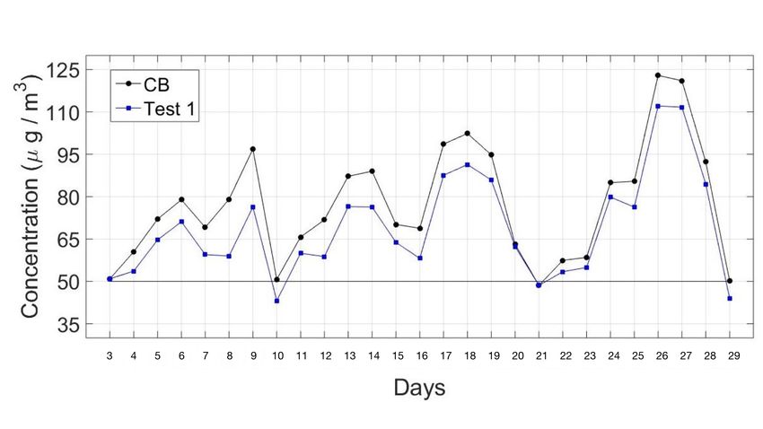
Electronics 2020, 9, 1409                                                                            2 of 17

      take into account both air quality levels and emission abatement costs using cost-effectiveness
      and/or multi-objective approaches [20–23]. They are also referred to as integrated assessment
      models (IAMs).

      This work is mainly focused on the introduction of a management tool for short-term policies
definition. This is a quite challenging task as in literature a series of IAMs has been described,
treating the problem in the long-term period and, for this reason, considering the atmosphere always
in a steady-state condition for the control problem solution [20,23–25].
      In this study, the implementation of a short-term integrated assessment model based on a receding
horizon technique is proposed. This approach can be used in two different configurations:

•     Scenario Mode: evaluation of the impact of a single set of actions on air quality;
•     Optimization Mode: selection of a set of (optimal) actions.

      The main advance with respect to literature is that considering the short-term (up to few days)
control problem means that the strong non-linearity of the system, and in particular its dynamics,
should be considered in control development. Moreover, to the authors knowledge, this is the first
time the receding horizon technique [26] is used for the development of air quality control.
      The implemented system has been tested on a domain in Northern Italy including Brescia city and
its surroundings, an area often affected by high PM10 (and other pollutants) concentrations, trying to
find an optimal set of actions to satisfy the PM10 concentration daily limits, minimizing, at the same
time, the application cost.

2. Methodology
    The short term IAM developed in this work is similar, in principles and structure, to existing long
term ones (Figure 1). In this figure, it is possible to identify the two key elements that are needed in an
IAM: a controller and a model, constituted by the comprehensive air quality model with eXtensions
(CAMx) model, optimal interpolation and correction factor (CF) blocks.

                                     Figure 1. Overall System Scheme.

     The choice of the CAMx [27] deterministic chemical transport model has been influenced by
the fact that short-term forecasting is driven by the dynamic of the phenomena involved and it is
usually strongly affected by uncontrollable variables, such as wind speed and precipitation rate.
These facts make the use of surrogate models less appealing due to their ability to represent with good
performances only the steady state of pollutants in atmosphere [28].
     Furthermore, to increase the model performance, a reanalysis technique based on an optimal
interpolation (OI) algorithm has been implemented. This allows to cope with input uncertainties
and approximation in the modelling of the different phenomena considered the model. In practice,
OI computes a correction factor (CF) by processing the last available measurements and model output
to improve forecast accuracy. Since in our case the last available measurements usually date back
to the day before the CTM forecast run, the only option is to hold the correction factor along the
prediction horizon.
Electronics 2020, 9, 1409                                                                                     3 of 17

     The controller has the goal to find a set of optimal emission abatement measures to be applied,
with respect to two main objectives: an air quality index and a cost index [29].

2.1. Problem Formulation
     Due to the nature of the involved phenomena, the control laws for the short-term air quality
control problem can be considered as a sequence of decisions taken by a (national, regional and/or
local) authority. In this work, the problem has been formalized through a multiple input, nonlinear
receding horizon control technique [26] where the control law ui acting on the horizon [i, i + N − 1],
with length N, is expressed as a sequence of M decisions (input):

                                    ui = {u1,i , ..., u M,i , ..., u1,i+ N −1 , .., u M,i+ N −1 }                (1)

    At each time step i an optimal control problem has to be solved and the first step of the solution
sequence ui is applied:

                                                                 i + N −1
                            min VN ( xk , ui , ·) = min
                              ui                            ui
                                                                   ∑        V ( xk , u1,k , ..., u M,k , ·)
                                                                   k =i
                            s. t.                                                                                (2)
                            xk+1 = f ( xk , uk , ·)              k = i, ..., i + N − 1
                             i
                            u ∈U

where:

•     VN is the objective function to be minimized, i.e., the sum of the objective functions V computed
      for each step. In this work, it includes both an air quality index and a cost index;
•     f ( xk , uk , ·) is the air quality model, allowing to estimate the evolution of the concentration of
      different pollutants in the atmosphere as a function of the concentration values computed at
      previous steps, the input controlled variable (emissions) and the uncontrolled ones (meteorology);
•     xk is the state of the system, i.e., the concentration of each species in each cell of the
      computational domain;
•     ui is the control sequence, as defined in Equation (1);
•     U is the feasible control set.

2.2. Control Sequence
     The control sequence ui represents the application of the different short term actions (STAs)
considered in the problem. The actions that can be included in the problem are short term abatement
measures that authorities/decision makers may implement to reduce atmospheric pollutant emissions.
In this work STAs are always binary (i.e., the action can be fully applied or not applied at all).
     STAs are defined in terms of:

•     Abatement factor: percentage emission reduction resulting from the application of an action
      on a domain cell. This factor depends on where the measure is applied, due to the presence
      of different drivers (emission activities) in different locations, i.e., wood burning reduction and
      traffic limitations do not have the same effect if applied in city centres or rural areas.
•     Application map: the area of application of an action. In order to keep considering uk as
      a binary value array, if a measure is applied on different areas, it will be considered as two
      separate measures.
•     Cost: implementing an STA has a cost that can be expressed both as a monetary or a social
      disappointment cost.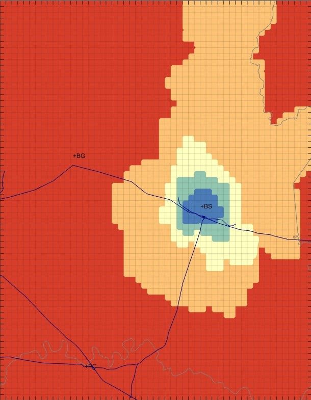
Electronics 2020, 9, 1409                                                                                                      4 of 17

     The pollutant emissions over the domain D are then a function of the control sequence ui
according to:
                                             d,p
                               Ed,p (ui ) = E0     1 − e f f (ui , p, d)                  (3)

where:

•     Ed,p is the emission value of pollutant p at cell d e D.
        d,p
•     E0 is the initial condition of the emission value, without the application of any of the abatement
      measures studied.
•     e f f is the effectiveness of the abatement measures applied for the control law ui , it represents how
      much the measures manage to reduce the given pollutant p at cell d.

2.3. Objective Function
     In Europe, in a typical short-term air quality management problem, a decision authority has
the task to keep the daily concentrations of a number of pollutants below the European Directive
thresholds, trying to minimize the impacts on the people affected by the application of the abatement
measures. A modelling system designed to solve this problem must take into account both these
aspects. Therefore, the objective function has to be composed by two functions to be minimized
simultaneously: the number of concentration exceedances and the monetary/social cost to implement
the emission abatement actions.
     In general, the objective function V (·) at time i will be expressed as:
                                                      "                #
                                                 i      Γ ( x k , ui )
                                       V ( xk , u ) =                                             (4)
                                                        Ω ( x k , ui )

where Γ and Ω are two real scalar functions allowing to compute the air quality index and the control
action cost over the chosen horizon.
     These values depend on the concentrations computed through the model, on the level of
application of the different actions and on the social costs of each single action.

2.4. Air Quality Forecast
     The most consistent way to proceed to define the function f that models the dynamic of the
pollutants in atmosphere consists in the use of full chemical transport models, allowing to threat all
the physical and chemical phenomena involved in emission, transport, accumulation and removal of
chemical species.
     In this work, the CAMx model [27] has been applied. CAMx is an open source chemical transport
model, based on Fortran source code, describing the physical and chemical phenomena involved in
the formation of pollutants solving the mass-balance Equation (5):

          ∂C
                 =     f Xtransport (·) + f Ytransport (·) + f Ztransport (·) + f XYdi f f usion (·) + f Zdi f f usion (·) +
          ∂t
                 +     f emission (·) + f deposition (·) + f chemistry (·)                                                        (5)

where C (µg/m3 ) is a vector composed by chemical species concentrations in ( x, y, z) at time t and the
different functions f ∗ are expressed in Equation (6):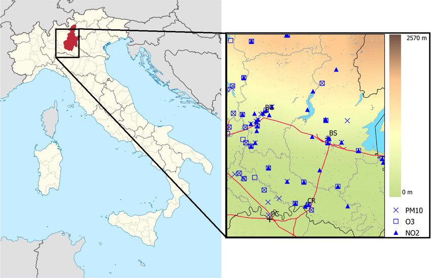
Electronics 2020, 9, 1409                                                                              5 of 17

                                  f emission        =   f em_mech ( E, ·)
                                                            1 ∂(uAyz C )
                                  f Xtransport      =   −
                                                           Ayz       ∂x
                                                           1 ∂(vA xz C )
                                  f Ytransport      = −
                                                          A xz  ∂y
                                                        ∂(Cη )       ∂2 h
                                  f Ztransport      =           −C                                        (6)
                                                           ∂z        ∂z∂t

                                                        ∂         ∂(C/ρ)
                                  f Zdi f f usion   =         ρKv
                                                        ∂z          ∂z

                                                         ∂        ∂(C/ρ)
                                 f XYdi f f usion   =         ρKx           +
                                                        ∂x           ∂x

                                                            ∂       ∂(C/ρ)
                                                        +       ρKy
                                                           ∂y          ∂y
                                  f deposition      =   −ΛC
                                  f chemistry       =   f chem_mech (·)

where Ayz and A xz (m2 ) represent, for each species, the cross-sectional areas in the y-z and x-z planes
respectively; the wind components in m/s on the horizontal plane are u (along direction x) and v (along
direction y); Kx , Ky and Kz denote the turbulent diffusion coefficient along the three dimensions; Λ is
the scavenging coefficients array [1/s] for each species; finally, f chem_mech (·) is the nonlinear function
illustrating the chemical transformations in atmosphere among the considered species according to
a selected chemical mechanism.
      As stated by Equation (6), a series of partial differential equation systems has to be solved. For this
reason the model needs in input the initial condition X0 and the boundary conditions xeast , xwest , xnorth ,
xsouth , xtop corresponding to the concentration values at the domain boundaries.
      Equations (6) can be solved by the model through different algorithms. The configuration applied
in this work is presented in Table 1.

                              Table 1. Selected configuration for CAMx model.

                                            Feature                       Options
                                  Chemical Mechanism                   CB05 [30,31]
                                    Advection Solver                    BOTT [32]
                                      Drydep Model                     WESELY [33]
                                    Chemistry Solver                     EBI [34]
                                    Aerosol Approach                     CF [27]
                            Inorganic Thermodynamic module           ISORROPIA [35]
                                 Organic Aerosol module                 SOAP [36]

     In general, the aerosol modules allow to take into account the aqueous chemistry, the partitioning
of inorganic aerosol constituents (sulphate, nitrate and ammonium) and gas-aerosol partitioning of
organics, allowing to include the most important processes in the formation and accumulation of
aerosol in atmosphere [27]. With these particular configurations, aerosol treatment is performed using
a coarse/fine approach, splitting the species in two different granulometries: coarse, with diameters
greater than 2.5 µ/m and fine, with diameters lower than 2.5 µ/m. The primary species (including
elemental and organic carbon) can be coarse or fine, while secondary species (nitrates, sulphates,
ammonium and secondary organic aerosols) are considered only as fine particles.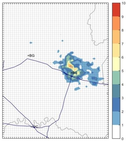
Electronics 2020, 9, 1409                                                                             6 of 17

     More details on air quality IAMs and CAMx can be obtained from [17,37]. Furthermore, an optimal
interpolation based data assimilation technique [38] has been integrated to reduce the effects of input
and model uncertainties on the system [39].

2.5. Optimal Interpolation
     Optimal Interpolation [13] is a reanalysis technique used to merge model simulations and
air quality measurements to obtain a more precise concentration field. The errors included in
measurements and forecasts can be represented as:

                                          Cb (t) = Ct (t) + ηb (t)                                       (7)
                                       y0 (t) = H(Ct (t)) + ε(t)                                         (8)

where:

•     Cb is the background simulated field (first guess), in this case, the output of the deterministic
      model CAMx.
•     Ct is the vector of true values.
•     ηb represents the error of the simulated values.
•     y0 is the observation vector that contains all the measurements.
•     H is a linear operator linking the grid field and the observations, typically bilinear interpolation
      is applied.
•     ε represents the error of the observations.

      This approach minimizes the error variance to compute a reanalyzed field Ca (t) according to:

                                   Ca (t) = Cb (t) + K[y0 (t) − H(Cb (t))]                               (9)

where K is known as the Kalman Gain and it is calculated as:

                                         K = PHT (HPHT + R)−1                                          (10)

      Based on the following statements:

•     P is the simulation errors covariance matrix.
•     R is the observation errors covariance matrix.
•     E[ηb ] = 0 and E[ε] = 0, thus both errors are unbiased.
•     E[ηb ε T ] = 0, thus the simulation errors are independent from the measurement ones.

     This methodology, according to [38] allows to obtain significant improvements in the precision of
deterministic model output for the simulation of PM10 daily mean concentrations.

3. Optimization Problem Solution
     This section describes in detail the procedure applied to solve the management problem described
in the previous sections. Three issues significantly affect the resolution:

•     to run the deterministic model CAMx is computationally expensive;
•     the huge number of input variables and relationships involved in CAMx to describe the
      phenomena of formation and accumulation of atmospheric pollutants makes the function
      modelled through the CTM model too complex to be studied;
•     the objective of the decision maker in the short-term period is to avoid/limit critical situation,
      i.e., the situation where the concentration values for a pollutant is higher than a critical threshold
      (usually defined at the legislative level).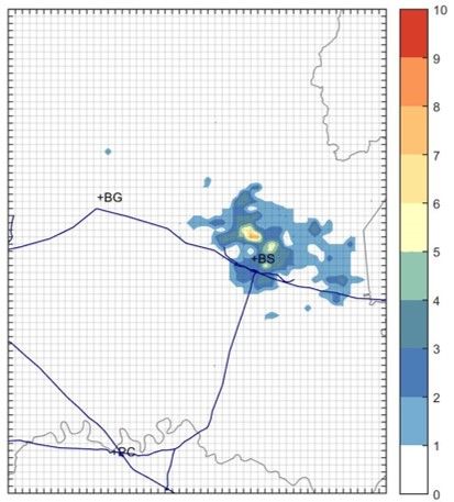
Electronics 2020, 9, 1409                                                                             7 of 17

     These facts strongly affect the implementation of the optimization procedure. Before the
presentation of the algorithm steps, three important features must be defined:

•     Forecast Horizon Window: it determines how many steps ahead the pollutant concentrations are
      forecasted. A wide forecast window will increase the model uncertainty and the computational
      burden for each cycle. However, abatement measures usually have a higher impact if applied
      in advance;
•     Application Interval Length: this determines for how many days, within the Forecast Horizon,
      the chosen actions are applied. In other words, it represents the actual control output length and
      the interval of time between subsequent IAM runs. This variable has a practical limitation, as its
      minimum value corresponds to running the IAM system and applying the optimal actions within
      the same day. This is highly unlikely to be obtained in a real life application for any authority.
      On the other hand, keeping this value as small as possible, allows the system to change the
      measures selection to cope with new, more accurate forecasts.
•     Measure Drop Threshold: This threshold determines the maximum air quality index degradation
      allowed during the optimization process, with respect to the best index value obtainable with the
      maximum application of all the measures. Thus, lower values will increase the weight of the air
      quality objective, higher values, instead, will increase the weight of the cost. For this work this
      value was set to 1.

     The optimization algorithm is based on a fast and simple heuristic procedure designed according
to the following steps:

1.     the control law ui is computed only if the air quality limit value is exceeded within the forecasting
       horizon window [i, i + N − 1];
2.     the control law computation starts with all the actions simultaneously applied for all the
       application interval length;
3.     each action is deactivated individually, and the impacts of these individual deactivations are
       assessed according to the following rules:

       •     exceedance days should not increase. If the deactivation of an action results in an increase,
             then the STA cannot be deactivated;
       •     the worsening of the air quality level, should be less than the value defined by the Measure
             Drop Threshold. If the worsening is higher, then the measure cannot be deactivated;
       •     the action with the highest cost among the ones respecting the previous rules is dropped.
             If two actions have the same cost, then the one with the highest air quality worsening
             is deactivated.
4.     the set of the resulting active STA is used as the base case for another iteration in order to
       deactivate other measures.
5.     finally, when no deactivation respects the previous control rules, the optimal set of actions
       is found.

     There is a special situation that needs extra consideration. When no air quality exceedances can
be found within the forecast horizon, no action is applied. Since the lack of exceedances may be caused
by prediction uncertainty then, the control system is run again the following day, without considering
the Application Interval length.

4. Case Study
     The methodology presented in the previous section has been applied to a particulate matter
(PM10 ) management case-study for the city of Brescia (Northern Italy) and its surrounding area.
The simulations presented in the following tests refer to January 2011 in order to apply the model to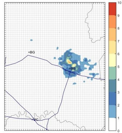
Electronics 2020, 9, 1409                                                                            8 of 17

an adverse situation, as Winter months in the selected area are characterized by frequent exceedances
of the daily average PM10 European Legislation threshold of 50 µg/m3 .

4.1. Case Study Setup
     The city of Brescia is one of the main urban centers in the Po valley basin and it is among the
European areas with higher particulate levels. The modelling domain is a 108 × 138 km2 area (Figure 2)
including almost all Brescia province as well as the neighboring cities of Cremona and Bergamo.
This area has been gridded into 3726 2 × 2 km2 squared cells. The meteorological fields are computed
by means of the weather research and forecasting (WRF) prognostic model [40], while the basecase
emission data are collected from the regional inventory INEMAR [41]. The boundary conditions
are obtained through a simulation performed with CAMx for the same period, but with a coarser
 6 × 6 km2 horizontal resolution over a domain covering the entire Northern Italy, following a one-way
nesting procedure. In this last case, the boundary conditions are obtained interpolating the results of
the Mozart global model [42]. More information and the validation of the simulation over the coarser
grid can be found in [37].

                 Figure 2. Modelling domain including the location of monitoring network stations.

4.2. Validation of Camx Model for PM10 Concentration
     A validation procedure has been applied in order to assess if CAMx can be used for the definition
of the control law. This validation was performed by comparing the output of the model with data
measured by the regional monitoring network (represented in Figure 2) following a Monte Carlo
approach as presented in [12]. With this approach a set of 100 re-analyses was performed using, for
each case, 80% of the stations for the optimal interpolation and the remaining 20% for the validation.
Figure 3 shows through boxplots the correlation coefficients (Figure 3a) and the normalized mean
absolute errors (Figure 3) computed for the validation stations on the domain. For the optimal
interpolation case, the worst performance index computed for each station in the 100 re-analyses was
considered. The results clearly showed the impact of the optimal interpolation techniques on the
model performances, with the median of the correlation increasing from 0.7 to a value close to 1 and
the median of normalized mean absolute error decreasing from 0.4 to less than 0.1. These figures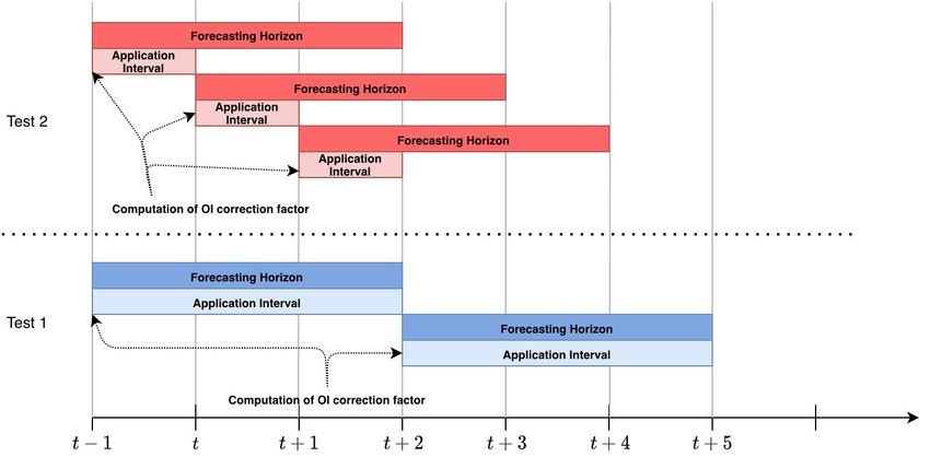
Electronics 2020, 9, 1409                                                                            9 of 17

highlight that the performance of CAMx, without optimal interpolation, was not enough to apply
the model for the definition of the control system, therefore, the following section will focus on the
application of the system integrating both CAMx and optimal interpolation.

                          (a)                                                    (b)
      Figure 3. PM10 daily mean concentration correlation coefficient (a) and normalised mean absolute
      error (b) for CAMx model and CAMx + optimal interpolation system.

4.3. Actions
     The actions considered in this work were specifically emission abatement measures focused on
the reduction of PM10 concentrations. Since PM has a primary (directly emitted) and a secondary
(formed in atmosphere) fraction, the measures included in the problem could affect directly primary
PM10 emissions and/or other precursors of secondary PM10 such as nitrogen oxides (NOx ).
     Each action was defined through three main variables:
1.     precursor abatement efficiency;
2.     application area;
3.     cost.
     In order to take into account the impact on PM10 concentrations in Brescia of the emission of
the surrounding areas, the domain was divided in three application zones as represented in Figure 4.
The smaller blue area included the cells belonging to the municipality of Brescia (Zone 1). The light
blue ring included Area 1 municipalities (Zone 2) defined according Lombardy region directives and
the outer yellow ring included Area 2 municipalities (Zone 3). Finally Zone 4 was composed by the
cells including highways and main streets (black line in Figure 4). The orange surrounding cells
highlight the whole province of Brescia, but were not considered for measure application in this work.

                            Figure 4. Application zone considered for the short term actions.

      The actions included in this case study were: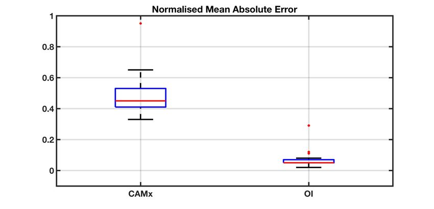
Electronics 2020, 9, 1409                                                                            10 of 17

•     Traffic Limitation/Car Ban: Traffic is among the main pollutant activities in the area, emitting
      significant quantities of NOx through internal combustion, primary PM from brakes and tires
      abrasion and particle re-suspension. In this short-term case study, traffic measures are applied
      with a limited time span (down to one day).
•     Maximum Speed Reduction: This action, if applied to highways and main streets, proved,
      in previous studies, to be a viable option to obtain concentration reductions near the streets [43],
      despite little influence at higher scales.
•     Heating Temperature Reduction: one degree reduction of indoor temperature. Even if the
      reduction factor is small, the area of application allows temperature reduction to cut a significant
      amount of emissions.
•     Wood Burning Limitation in the area under study 98% of domestic heating emissions comes from
      biomass burning. Long term limitations are already in place, but further emergency limitations
      are expected to effectively contribute to particulate concentration reductions.
      Table 2 presents all the measures considered with the values assigned to their properties.
Application efficiency values have been extracted from INEMAR database [41]. Costs are extremely
difficult to compute. In first instance, and in absence of better criteria, the cost of each action has been
computed as a “dissatisfaction estimate” based on the amount of population affected by the measure.

                                     Table 2. Abatement measures available.

                            Action          Zone    PM10 Reduction     NOx Reduction    Cost
                     Traffic Limitation       1           42%                 51%        2
                     Traffic Limitation       2           25%                 52%        3
                     Traffic Limitation       3           25%                 52%        5
                     Speed Reduction          4           23%                  5%        2
                      Reduce Heating          3           5%                  5%         2
                  Wood Burning Limitation     1           30%                 4%         2
                  Wood Burning Limitation     2           50%                 7%         3
                  Wood Burning Limitation     3           50%                 7%         4

4.4. Objective Function and Control Law Definition
      In this work, according to Equation (4), the selected objective function Γ is the number of the
days, over Zone 1, with the daily mean concentration of PM10 higher than the legislation threshold of
50 µg/m3 (European legislation index for PM10 ). Ω objective function, taking into account the cost of
the control law, is simply the sum of the daily costs of each selected action.
      Following the decision to use a threshold index for air quality, the general optimization problem
solution procedure was adapted in order to consider an action as a candidate for deactivation, not only
if the resulting worsening of the concentration levels was under the Measure Drop Threshold, but also
if the number of exceedance days did not increase after the deactivation. Moreover, a constraint
related to the decision level was considered in the solution: in order to be activated for an outer zone,
the action also had to be applied to the inner zones.

4.5. Results
      The results obtained through the previous methodology were assessed by comparing avoided
PM10 exceedances and daily average PM10 concentrations with a maximum reduction scenario
(referred as Test Max in the following subsections) built by always applying all the measures available.
Two different configurations of the system were tested:
•     Test 1: applies the IAM (with control) with a three day forecast horizon and keeping the application
      of the resulting measures fixed for the next three days. Optimal interpolation is based on the
      measurements of the day before the IAM run. This test simulates a situation in which the decision
      maker cannot change the strategy every day;
Electronics 2020, 9, 1409 11 of 17
• Test 2: applies the daily IAM (with control) with a three day forecast horizon. In this case the pool
of measures applied varies every day. This is the standard implementation of the receding horizon
technique, but it implies that the decision makers can impose every day different measures to the
population. Optimal interpolation is based again on the measurements of the day before each
IAM run;
The scheme in Figure 5 allows us to better appreciate the differences in the two configurations.
Assuming that the decision maker required the computation of the control law at time t − 1 (when the
last measurement was available for optimal interpolation), both the systems performed a 3-days-ahead
forecast in order to compute the control actions to be activated for each day in the interval t ÷ t + 2.
In the first case (Test 1), the solution was applied for the entire interval. In the second configuration
(Test 2), the actions were applied for the first day of the interval and a new 3-days-ahead forecast
was performed, once the correction factor was updated with new available measurements (day t).
The second configuration (very similar to a classical receding horizon approach) ensured a better
forecast thanks to the use of correction factors that were updated every day, but had a higher
computational cost. It is, therefore, a good benchmark for the performances of the Test 1.
Figure 5. Differences between Test 1 and Test 2 configuration.
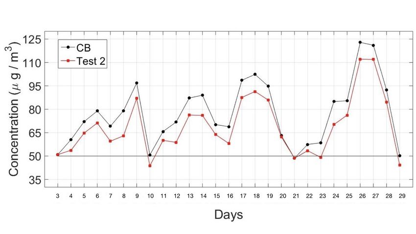
Figure 6 presents the daily mean PM10 concentrations for the 3 different tests over the period
under study (January 2011). From the results of the Test Max configuration (the test performed with
all the measures activated) it is possible to see that the problem was quite difficult to solve, since also
in this potential application scenario, the reduction of the exceedance days was limited. Moreover,
it seems that the impact of the selected actions was not enough to consistently change the dynamic
of the phenomena and that a stronger carrier was affecting the system as an uncontrolled input.
Nevertheless, in the three cases the controlled PM10 concentrations were very similar, with the exception
of days 21–23. In these days, only the Test Max configuration was able to avoid any exceedance,
while Test 1 and Test 2 could not always push the PM10 levels under the threshold. This is probably
due to the fact that the the concentration values, in these days, were close to the threshold, thus, even a
small forecast error could drastically change the behaviour of the optimization algorithm. For what
the Test 1 and Test 2 is concerned, the main difference between the results of them was that the higher
dynamic of Test 2 configuration allowed us to avoid an exceedance for day 23. Furthermore, on day
9, Test 1 (and Test Max) ensured a higher concentration reduction (around 20 µg/m3 ) with respect to
Test 2. This is due (1) to the fact that Test 2, due to its dynamic, was able to capture the concentration
decrease for the following day and (2) to the optimization procedure aiming to reduce the exceedancesElectronics 2020, 9, 1409 12 of 17
with the minimum effort, so, no action is taken when a non exceedance day was forecasted. In Test 1,
instead, all the measures were kept in place due to the 3-day application constraint.
(a)
(b)
(c)
Figure 6. Particulate matter (PM10 ) concentration before (CB) and after the actions for Test 1 (a), Test 2
(b) and Test Max (c).
Figure 7 presents, for each day, the measures application resulting from Test 1 (Figure 7a) and 2
(Figure 7b). It is possible to see that Test 2 had an obvious higher variability in the activation of the
measures and, in days 9, 20 and 21 few or no measures were applied, allowing the final policy cost toElectronics 2020, 9, 1409 13 of 17
decrease. In Test 1, the 3-day choice constraint was clearly recognizable in the pattern. This Figure
also confirms that the constraint inhibits the possible temporary deactivation of the measures seen in
Test 2 for day 9, delays the deactivation of measures for day 20 and the subsequent reactivation two
days later.
(a)
(b)
Figure 7. Resulting measure application for Test 1 (a) and Test 2 (b) for each day.
Table 3 presents, for the different tests performed, the number of exceedances with respect to the
50 µg/m3 threshold, the measure application costs, and the monthly mean PM10 concentrations.
Table 3. Results Comparison.
Test Exceedances Cost PM10
Base Case 26 0 77.5
Test 1 24 268 69.0
Test 2 23 253 69.0
Test Max 21 351 67.3
The best result with respect to air quality (minimum number of exceedances and particulate
matter concentration) was obviously obtained at the maximum cost for the maximum application
scenario. This also established that with the current pool of measures the IAM could reduce the
maximum 5 exceedance days for the current case study; still, building a IAM that helped to reach this
5-day reduction at the minimum cost can be extremely helpful in order to reach the 35 exceedance
days limit required by the legislation.
The differences between Test 1 and 2 showed how an improvement in the dynamic capability of
the control system (daily IAM run instead of 3 days’ run) could improve the air quality and reduce the
cost of the strategies.
As can be observed by mapping the reduction in exceedance days as in Figure 8, all the tests
managed to achieve reductions, with a maximum of 10 days reduction for some cells located North
of Brescia. It is important to notice how, for Test 1 and Test Max, where the actions applied were
kept for several days, there are reductions reaching areas further from the city with respect to Test 2
where the actions are redefined everyday. These representation aids the comprehension of the resultsElectronics 2020, 9, 1409 14 of 17
previously presented in Table 3 and shows how, for example, Test 2 obtains higher reductions in the
cells of interest (Zone 1) with respect to Test 1. Finally, 1 day reductions located in sparse cells outside
the domain are due to computational approximations.
Test 1 Test 2 Test Max
Figure 8. Map of exceeded days reduction.
5. Conclusions
The objective of this work was to implement and test a short term integrated assessment model
to aid decision makers in the definition of short term plans (STPs) to reduce peak particulate matter
concentration and the number of exceedance days with respect to thresholds values defined in
the legislation.
In literature, many different long term decision support systems can be found. These systems
tend to focus on the reduction of mean pollutant concentration values for wide temporal windows
(usually annual) considering a steady state system. These IAMs are not able to handle daily variations
in emissions and concentrations as a short term IAM, instead, should do. Furthermore, uncontrolled
variables as weather conditions must be included in the latter problem as they have huge impacts on
the daily variations of particulate matter concentration.
The IAM described in this paper is composed of a deterministic model coupled with an optimal
interpolation algorithm to feed a nonlinear receding horizon controller able to select the optimal sets
of short term emission abatement actions. The IAM, tested on a case-study for the month of January
2011 over the city of Brescia, managed to obtain cost-efficient strategies resulting in a reduction of
2 and 3 days of exceedance, depending on the configuration. This result should be seen in the light of
a 5 days potential reduction obtained with the maximum application of all the actions considered in
the problem.
A number of considerations arise from the case-study results:
• Running the IAM every day increases the computational burden and leaves little notification time
for a real world application, but it allows to obtain better results with respect to occasional IAM
runs for wider time windows. Further studies should be done in order to determine the best
forecast window and running frequency combination to enhance the controller performance.
• PM10 exceedances forecasting is a challenging problem. Even if the overall performances of the
CAMx model are good (in particular in combination with the implemented optimal interpolation
technique), little deviations with respect to the measured values can consistently affect the
performances, in particular when values are close to the threshold.
• The actions applied in order to reduce particulate matter concentration only over the city of
Brescia, also resulted in an air quality improvement for the surrounding areas.
• Further studies should be done in order to add variability to the cost index to take into account
the disadvantages arising from last minute notification to the population. This also implies the
need of a better model in order to predict further in time.Electronics 2020, 9, 1409 15 of 17
• Long term actions effects (such as those arising from regional plans) should be included in the
problem allowing to evaluate the combined effects with the short term actions selected by the
short term IAM.
Author Contributions: Conceptualization, C.C., E.D.A., F.L.T., E.T. and M.V.; data curation, E.D.A. and
E.T.; funding acquisition, M.V.; methodology, C.C. and F.L.T.; software, F.L.T. and E.T.; validation, C.C.;
writing—original draft, C.C., F.L.T. and E.T. All authors have read and agreed to the published version of
the manuscript.
Funding: This research received no external funding.
Conflicts of Interest: The authors declare no conflict of interest.
References
1. Landrigan, P.; Fuller, R.; Acosta, N.; Adeyi, O.; Arnold, R.; Basu, N.; Baldé, A.; Bertollini, R.; Bose-O’Reilly, S.;
Boufford, J.; et al. The Lancet Commission on pollution and health. Lancet 2018, 391, 462–512. [CrossRef]
2. Pope, C., III; Dockery, D.; Spengler, J.; Raizenne, M. Respiratory health and PM10 pollution: A daily time
series analysis. Am. Rev. Respir. Dis. 1991, 144, 668–674. [CrossRef]
3. Pope, C., III; Dockery, D. Acute health effects of PM10 pollution on symptomatic and asymptomatic children.
Am. Rev. Respir. Dis. 1992, 145, 1123–1128. [CrossRef] [PubMed]
4. Miranda, A.; Silveira, C.; Ferreira, J.; Monteiro, A.; Lopes, D.; Relvas, H.; Borrego, C.; Roebeling, P. Current
air quality plans in Europe designed to support air quality management policies. Atmos. Pollut. Res. 2015,
6, 434–443. [CrossRef]
5. Manerba, D.; Mansini, R.; Zanotti, R. Attended Home Delivery: Reducing last-mile environmental impact
by changing customer habits. IFAC Pap. 2018, 51, 55–60. [CrossRef]
6. Zhang, M.; Shan, C.; Wang, W.; Pang, J.; Guo, S. Do driving restrictions improve air quality: Take
Beijing-Tianjin for example. Sci. Total Environ. 2020, 712, 136408. [CrossRef]
7. Giannouli, M.; Kalognomou, E.A.; Mellios, G.; Moussiopoulos, N.; Samaras, Z.; Fiala, J. Impact of European
emission control strategies on urban and local air quality. Atmos. Environ. 2011, 45, 4753–4762. [CrossRef]
8. Li, L.; Zheng, Y.; Zheng, S.; Ke, H. The new smart city programme: Evaluating the effect of the internet of
energy on air quality in China. Sci. Total Environ. 2020, 714, 136380. [CrossRef]
9. Turrini, E.; Vlachokostas, C.; Volta, M. Combining a Multi-Objective Approach and Multi-Criteria Decision
Analysis to Include the Socio-Economic Dimension in an Air Quality Management Problem. Atmosphere 2019,
10, 381. [CrossRef]
10. Marques, G.; Pires, I.M.; Miranda, N.; Pitarma, R. Air Quality Monitoring Using Assistive Robots for
Ambient Assisted Living and Enhanced Living Environments through Internet of Things. Electronics 2019,
8, 1375. [CrossRef]
11. Arroyo, P.; Lozano, J.; Suárez, J. Evolution of Wireless Sensor Network for Air Quality Measurements.
Electronics 2018, 7, 342. [CrossRef]
12. Carnevale, C.; Finzi, G.; Pederzoli, A.; Pisoni, E.; Thunis, P.; Turrini, E.; Volta, M. A methodology for
the evaluation of re-analyzed PM10 concentration fields: A case study over the PO Valley. Air Qual.
Atmos. Health 2015, 8, 533–544. [CrossRef]
13. Candiani, G.; Carnevale, C.; Finzi, G.; Pisoni, E.; Volta, M. A comparison of reanalysis techniques: Applying
optimal interpolation and Ensemble Kalman Filtering to improve air quality monitoring at mesoscale.
Sci. Total Environ. 2013, 458–460, 7–14. [CrossRef] [PubMed]
14. Grivas, G.; Chaloulakou, A. Artificial neural network models for prediction of PM10 hourly concentrations,
in the Greater Area of Athens, Greece. Atmos. Environ. 2006, 40, 1216–1229. [CrossRef]
15. San José, R.; Pérez, J.L.; Morant, J.L.; González, R.M. European operational air quality forecasting system by
using MM5–CMAQ–EMIMO tool. Simul. Model. Pract. Theory 2008, 16, 1534–1540. [CrossRef]
16. Manders, A.; Schaap, M.; Hoogerbrugge, R. Testing the capability of the chemistry transport model
LOTOS-EUROS to forecast PM10 levels in the Netherlands. Atmos. Environ. 2009, 43, 4050–4059. [CrossRef]
17. Carnevale, C.; De Angelis, E.; Finzi, G.; Turrini, E.; Volta, M. An integrated forecasting system for air quality
control. In Proceedings of the 2019 18th European Control Conference, ECC 2019, Naples, Italy, 25–28 June
2019; pp. 830–835.Electronics 2020, 9, 1409 16 of 17
18. Ou, Y.; Shi, W.; Smith, S.J.; Ledna, C.M.; West, J.J.; Nolte, C.G.; Loughlin, D.H. Estimating environmental
co-benefits of U.S. low-carbon pathways using an integrated assessment model with state-level resolution.
Appl. Energy 2018, 216, 482–493. [CrossRef]
19. Qiu, X.; Zhu, Y.; Jang, C.; Lin, C.J.; Wang, S.; Fu, J.; Xie, J.; Wang, J.; Ding, D.; Long, S. Development of an
integrated policy making tool for assessing air quality and human health benefits of air pollution control.
Front. Environ. Sci. Eng. 2015, 9, 1056–1065. [CrossRef]
20. Turrini, E.; Carnevale, C.; Finzi, G.; Volta, M. A non-linear optimization programming model for air quality
planning including co-benefits for GHG emissions. Sci. Total Environ. 2018, 621, 980–989. [CrossRef]
21. Carnevale, C.; Ferrari, F.; Guariso, G.; Maffeis, G.; Turrini, E.; Volta, M. Assessing the Economic and
Environmental Sustainability of a Regional Air Quality Plan. Sustainability 2018, 10, 3568. [CrossRef]
22. Gimez Vilchez, J.; Julea, A.; Peduzzi, E.; Pisoni, E.; Krause, J.; Siskos, P.; Thiel, C. Modelling the impacts
of EU countries electric car deployment plans on atmospheric emissions and concentrations. Eur. Transp.
Res. Rev. 2019, 11, 40. [CrossRef]
23. Relvas, H.; Miranda, A.; Carnevale, C.; Maffeis, G.; Turrini, E.; Volta, M. Optimal air quality policies and
health: A multi-objective nonlinear approach. Environ. Sci. Pollut. Res. 2017, 24, 13687–13699. [CrossRef]
[PubMed]
24. Pisoni, E.; Thunis, P.; Clappier, A. Application of the SHERPA source-receptor relationships, based on the
EMEP MSC-W model, for the assessment of air quality policy scenarios. Atmos. Environ. 2019, 4, 100047.
[CrossRef]
25. Thunis, P.; Degraeuwe, B.; Pisoni, E.; Meleux, F.; Clappier, A. Analyzing the efficiency of short-term air
quality plans in European cities, using the CHIMERE air quality model. Air Qual. Atmos. Health 2017,
10, 235–248. [CrossRef] [PubMed]
26. Grune, L.; Pannek, J. Nonlinear Model Predictive Control—Theory and Algorithms; Springer: Berlin/Heidelberg,
Germany, 2011.
27. Ramboll Environment and Health. CAMx User’s Guide Version 6.50; Technical Report; Ramboll Environment
and Health: Copenhagen, Denmark, April 2018.
28. Carnevale, C.; Finzi, G.; Guariso, G.; Pisoni, E.; Volta, M. Surrogate models to compute optimal air quality
planning policies at a regional scale. Environ. Model. Softw. 2012, 34, 44–50. [CrossRef]
29. Carnevale, C.; Pisoni, E.; Volta, M. Formalizing and solving the PM10 control problem. In Proceedings of
the 17th World Congress, the International Federation of Automatic Control, Seoul, Korea, 6–11 July 2008.
30. Whitten, G.Z.; Heo, G.; Kimura, Y.; McDonald-Buller, E.; Allen, D.T.; Carter, W.P.; Yarwood, G. A new
condensed toluene mechanism for Carbon Bond: CB05-TU. Atmos. Environ. 2010, 44, 5346–5355. [CrossRef]
31. Yarwood, G.; Rao, S.; Yocke, M.; Whitten, G. Updates to the Carbon Bond Chemical Mechanism: CB05;
Final Report; US-EPA: Washington, DC, USA, 2005.
32. Bott, A. Improving the time-splitting errors of one-dimensional advection schemes in multidimensional
applications. Atmos. Res. 2010, 97, 619–631. [CrossRef]
33. Wesely, M.; Hicks, B. A review of the current status of knowledge on dry deposition. Atmos. Environ. 2000,
34, 2261–2282. [CrossRef]
34. Hertel, O.; Berkowicz, R.; Christensen, J.; Hov, Ã. Test of two numerical schemes for use in atmospheric
transport-chemistry models. Atmos. Environ. Part Gen. Top. 1993, 27, 2591–2611. [CrossRef]
35. Fountoukis, C.; Nenes, A. ISORROPIAII: A computationally efficient thermodynamic equilibrium model for
K+-Ca2 +-Mg2 +-NH4 +-Na+-SO42 -NO3 -Cl-H2 O aerosols. Atmos. Chem. Phys. 2007, 7, 4639–4659. [CrossRef]
36. Strader, R.; Lurmann, F.; Pandis, S. Evaluation of secondary organic aerosol formation in winter.
Atmos. Environ. 1999, 33, 4849–4863. [CrossRef]
37. Carnevale, C.; Angelis, E.; Finzi, G.; Pederzoli, A.; Turrini, E.; Volta, M. A non linear model approach to
define priority for air quality control. IFAC Pap. 2018, 51, 210–215. [CrossRef]
38. Candiani, G.; Carnevale, C.; Filisina, V.; Finzi, G.; Pisoni, E.; Volta, M. Optimal interpolation to
re-analyse PM10 concentration modelling simulations. In Proceedings of the 48th IEEE Conference on
Decision and Control (CDC) Held Jointly with 2009 28th Chinese Control Conference, Shanghai, China,
15–18 December 2009; pp. 1794–1799.
39. Carnevale, C.; Douros, J.; Finzi, G.; Graff, A.; Guariso, G.; Nahorski, Z.; Pisoni, E.; Ponche, J.L.; Real, E.;
Turrini, E.; et al. Uncertainty evaluation in air quality planning decisions: A case study for Northern Italy.
Environ. Sci. Policy 2016, 65, 39–47. [CrossRef]Electronics 2020, 9, 1409 17 of 17
40. Skamarock, W.C.; Klemp, J.; Dudhia, J.; Gill, D.O.; Barker, D.M.; Duda, M.G.; Huang, X.Y.; Wang, W.; Powers, J.G.
A Description of the Advanced Research WRF Version 3; Note NCAR/TN-475+STR; NCAR: Boulder, CO, USA, 2008.
41. ARPA Lombardia. INEMAR—Lombardy Region Emission Inventory. 2011. Available online: http:
//www.inemar.eu (accessed on 21 January 2016)
42. Emmons, L.K.; Walters, S.; Hess, P.G.; Lamarque, J.F.; Pfister, G.G.; Fillmore, D.; Granier, C.; Guenther, A.;
Kinnison, D.; Laepple, T.; et al. Description and evaluation of the Model for Ozone and Related chemical
Tracers, version 4 (MOZART-4). Geosci. Model Dev. 2010, 3, 43–67. [CrossRef]
43. Hodges, N.; Obzynska, D.J.; Lad, D.C.; Swaton, R. Air Quality Management Guidebook; Technical Report,
Citeair—INTERREG 3C Project. 2005. Available online: http://citeair.rec.org/downloads/Products/
AirQualityManagement.pdf (accessed on 2 May 2020).
c 2020 by the authors. Licensee MDPI, Basel, Switzerland. This article is an open access
article distributed under the terms and conditions of the Creative Commons Attribution
(CC BY) license (http://creativecommons.org/licenses/by/4.0/).You can also read