Physical Modelling vs. Numerical Modelling: Complementarity and Learning - Preprints.org

Preprints (www.preprints.org) | NOT PEER-REVIEWED | Posted: 31 July 2020 doi:10.20944/preprints202007.0753.v1

 Article

 Physical Modelling vs. Numerical Modelling:
 Complementarity and Learning
 José S. Antunes do Carmo
 Department of Civil Engineering, University of Coimbra, 3030-788 Coimbra, Portugal; jsacarmo@dec.uc.pt;
 Tel.: +351-239-797-153

 Abstract: We are witnessing a progressive divestment of some institutions with strong traditions
 and skills in physical modelling and their consequent impoverishment, to the detriment of
 numerical modelling. For many reasons, the economic imperatives and the exponential growth of
 computational means and numerical methods should certainly not be excluded. In this work, we
 aimed to highlight the new requirements of the recent sophisticated developments in physical
 modelling, precisely due to the new needs imposed on them by mathematical and numerical
 modelling and the growing risks in civil construction works. In this context, reflections are reported,
 justified by scientific and real-world examples, on the need for maintenance and reinforcement of
 investments in physical modelling, both to support the scientific community and to design buildings
 of significant economic, social and environmental impact.

 Keywords: physical modelling; numerical modelling; construction works; growing risks; safety
 requirements; hybrid modelling

 1. Introduction
 Model studies can be useful for academic and scientific purposes and to explain a project to
 stakeholders and the public in real-world applications. They are important for the design and
 verification of construction works with significant dimensions, costs and impacts, whether numerical
 models or physical models.
 Research on turbulence, waves, soil– and fluid–structure interaction, among others, have been
 carried out for a long time by different approaches, such as analytical solutions [1,2], laboratory
 measurements or comparison of both the experimental findings and field data [3,4] and, more
 recently, numerical modelling and hybrid experimental and numerical modelling [5–7].
 Until the 1970s, the first two approaches (analytical solutions and physical modelling) were the
 only ones widely used. At that time, physical modelling techniques were widely used in different
 fields.
 Since then, as reported by Carmo [8], not only has our theoretical knowledge of the phenomena
 improved greatly, the way we use numerical methods has also become more efficient. The great
 advances made in computer technology, especially since the 1980s, e.g., improving information
 processing and enabling large amounts of data to be stored, have made possible the use of
 mathematical models of greater complexity and with fewer restrictions. This led to the widespread
 use of numerical modelling to the detriment of the other two approaches.
 Currently, in some fields, numerical modelling appears to be more advantageous. An example
 is the ability to predict the evolution and behaviour of oil spilled at sea, regardless of the atmospheric
 conditions. To help estimate the ecological risks of oil spill contamination and potential hypoxia,
 rapid, efficient, accurate and timely detection is required to determine where, when and how to carry
 out response plans. This is intrinsic to the numerical models. In preventive terms, numerical models
 could even be the only viable solution to plan any implementation to combat pollution at sea [9,10].
 Climatology is a field in which numerical modelling is the only means of simulation, particularly
 weather and climate forecasts for time scales ranging from a few weeks to a few decades into the

 © 2020 by the author(s). Distributed under a Creative Commons CC BY license.

Preprints (www.preprints.org) | NOT PEER-REVIEWED | Posted: 31 July 2020 doi:10.20944/preprints202007.0753.v1

 future (sub-seasonal to decadal climate prediction). These models work by integrating data (surface
 and upper-air observations of temperature, pressure, moisture, winds and air density) into equations
 that are solved numerically. As more and more types of data are assimilated into the models, the
 quality of the model forecasts often improves [11].
 Numerical models are all the more useful the better they represent the real problem, but this is
 not always possible, or it is possible but with more or fewer simplifications. Despite the huge
 developments in numerical models, they still have limitations or gaps in the reproduction of many
 physical phenomena, especially when applied to complex flows, such as turbulent flows [12,13],
 fluid–structure interaction [14,15], breaking waves, etc.
 A numerical model will be attractive and can solve a fluid–structure interaction (FSI) problem if
 it verifies the following properties: (1) the mathematical model has FSI capability; (2) the scheme is
 sufficiently robust and works without fail for a reasonable period; (3) the solution is accurate and
 proven analytically and/or experimentally; (4) the model is efficient within a reasonable computation
 time.
 Thanks to the technological revolution that occurred in the last few decades, new physical
 perspectives have arisen due to the development of new sophisticated equipment and the great
 improvement of experimental techniques, thus allowing us to overcome the limitations of numerical
 modelling [16].
 In fact, given the new experimental techniques, physical modelling allows for the study of new
 phenomena and the measurement of variables in complex flows inaccessible by theory. Physical
 modelling also allows us to confirm theoretical results, analyse different details of a project and test
 a wide variety of environmental and extreme conditions [17].
 Another field in which physical modelling plays an essential role, by allowing us to calibrate
 and validate parametric formulations, is the scour process around bridge piles. The settlement of
 marine structures due to the littoral dynamics is another process induced by scouring around their
 foundations [18]. Due to the action of currents and waves, these processes have become the main
 factors that affect the safety of the construction and operation of bridge foundations and other
 structures in rivers, coastal and offshore environments [19].
 Today’s automated data acquisition and analysis systems, fast processing and increased data
 storage capabilities provide significant uses for the validation of numerical models [20]. In this
 context, physical modelling has been fundamental for the study of processes related to turbulent
 phenomena, allowing for the validation of current turbulence models, e.g., the two-equation models
 k-ε, RNG k-ε and k-ω [21].
 Although physical models have several advantages, they also have several difficult-to-solve
 problems, such as scale effects, because it is impossible to correctly scale a free-surface hydrodynamic
 model using water that satisfies all of the laws of similitude, laboratory effects, due to reflection and
 flow restriction, duration of tests, incomplete modelling and installation and maintenance costs [22].
 As reported in [23], physical models can be used in conjunction with numerical models as a
 hybrid model to take advantage of each model’s benefits. In a hybrid model, one can have numerical–
 physical or physical–numerical model connectivity. For instance, the numerical model is used to
 provide input to the physical model which then provides its output as input to the same or another
 numerical model.
 The complementarity of physical and numerical modelling is a very rich field to be explored in
 terms of teaching engineering, both in the laboratory and in the classroom. The information obtained
 from numerical models and experimental results is crucial for the development of an understanding
 of the behaviour of actual structures and methods to efficiently design them; therefore, the promotion
 of practical lessons based on physical and numerical models is critically important.
 The use of physical models can help to improve our understanding of how structures work. It is
 important to remember that both physical models and numerical models are good options as long as
 they are an accurate representation of the actual structure [24]. To illustrate various physical aspects
 of seepage in dams, Marques [25] shows the advantages of numerical modelling in the geotechnical
 training of civil engineering students.

Preprints (www.preprints.org) | NOT PEER-REVIEWED | Posted: 31 July 2020 doi:10.20944/preprints202007.0753.v1

 In this paper, the advantages and disadvantages of each of the physical and numerical
 simulations are shown through academic/scientific examples and real-world applications. The
 complementarity virtues of both methodologies are then demonstrated via the teaching, learning,
 improvement or development of theoretical models and the calibration/validation of empirical-based
 methods.
 Section 2 details and discusses the laboratory experiments used to validate semi-empirical
 models and to assess the behaviour of large-scale structures, where physical modelling is useful to
 complement or improve the results of numerical modelling. Inefficient or inappropriate uses of
 numerical models and physical modelling to improve mathematical models, so that they can describe
 the most important phenomena with enough approximation, are shown in Section 3. A final
 discussion is provided in Section 4.

 2. Materials and Methods
 In general, a physical modelling test program needs a high number of experiments; however,
 physical modelling tests are time-consuming and expensive. Numerical modelling plays an
 important role in countering this requirement as they can help to interpret the experimental results
 and, thus, reduce the number of tests to be performed. In addition to physical modelling performed
 in the laboratory, a numerical model is a valuable tool for the analysis and explanation of phenomena
 in different fields.
 In the field of soil mechanics, the use of physical modelling is common, especially to assess the
 soil–structure interaction phenomena and to validate semi-empirical models. Figure 1 provides a
 general view of an experiment of a study carried out in a laboratory by [18] to investigate the scour-
 settlement process of vertical cylindrical piles of differing heights and densities.

 Figure 1. General view of an experiment from a study carried out in the laboratory.

 Numerical modelling is not capable of reproducing the phenomena that occur in these
 circumstances in the way that physical modelling can. As reported in [18], experiments on the local
 scour produced by regular and nonlinear waves around a single pile have shown a good fitting between
 the equilibrium scour depth S and the Keulegan–Carpenter number. We found that it was possible
 to test and validate model (1), which seems to provide a good representation of the scour S.
 
 = 1.3 [1 − −0.06( −6) ] (1)
 
 where D is the diameter of the cylindrical pile, and KC is the Keulegan–Carpenter number, as defined
 in [18].

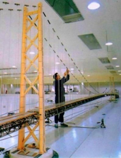
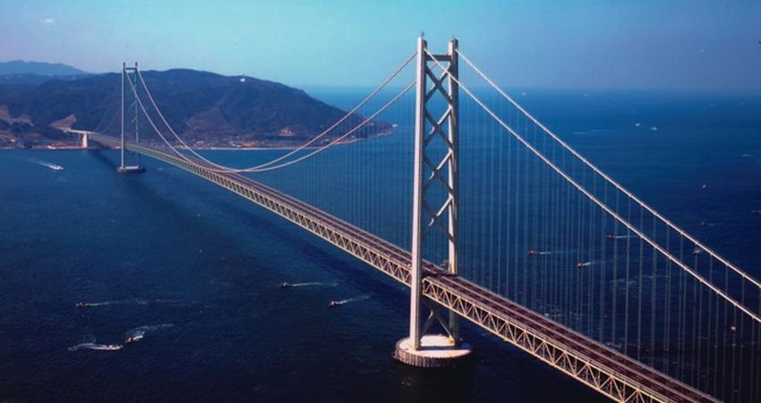
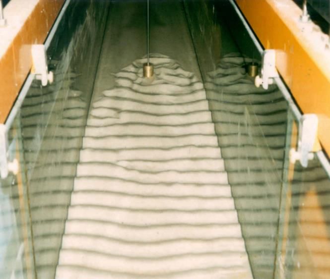
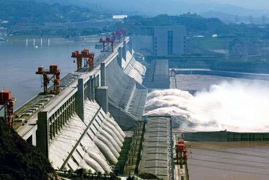
Preprints (www.preprints.org) | NOT PEER-REVIEWED | Posted: 31 July 2020 doi:10.20944/preprints202007.0753.v1

 In the area of structural mechanics, it is mainly the construction of bridges and concrete and
 earth-fill dams that require complementary physical and numerical simulation approaches to assess
 specific aspects of design, construction, and structural behaviour of different types of actions/forcing.
 We refer the reader to the works of Chen and Chen [26], Al-Janabi et al. [27] and Ninot et al. [28],
 among many others for more information on this topic.
 Relevant real-world examples of complementarity between physical and numerical approaches
 in the design phase are the Akashi Kaikyo Bridge (Japan) (Figure 2) [29] and the Three Gorges Dam
 (currently the world’s largest dam, capacity 39.3 km3, China) shown in Figure 3 [30].

 Figure 2. Longest suspension bridge in the World—Akashi Kaikyo Bridge, Japan [29].

 Figure 3. Currently the world’s largest dam—The Three Gorges Dam, China [30].

 The physical model of the Akashi Kaikyo Bridge in a Wind Tunnel is shown in Figure 4 [31],
 where it was subjected to experimental testing—to varying wind speeds and loading. The physical
 model of the no. 3 powerhouse-dam section of the Three-Gorges Dam is shown in Figure 5 [32].

Preprints (www.preprints.org) | NOT PEER-REVIEWED | Posted: 31 July 2020 doi:10.20944/preprints202007.0753.v1

 Figure 4. Akashi Kaikyo Bridge model in a wind tunnel [31].

 Figure 5. Physical model of no. 3 powerhouse-dam section [32].

 Numerous papers were published describing the physical modelling and experimental results
 from testing of the model (e.g., [33,34]).
 To analyse the bridge’s response to wind action and ensure that it functions correctly under
 stress, an interesting description of the types of tests generally performed in a wind tunnel at the
 design stage is provided in [35,36]. A comparison of the maximum static horizontal deflection of the
 Akashi bridge with that of the Messina Bridge (Italy) is also discussed.
 Both the numerical and physical modelling tests of the Three Gorges Dam have demonstrated
 that the stability against sliding of the critical dam section (the no. 3 powerhouse-dam section) can
 meet the safety requirements [37,38], and the following conclusion was drawn, “The integration of
 multiple methods is shown to be a more effective approach for the stability analyses of the Three-
 Gorges Dam foundation since no satisfactory individual method can be used alone to solve the
 problem”.
 Within the scope of fluid mechanics, there are several references for the need to complement
 different analysis methodologies, highlighting the phenomena of turbulence, fluid–structure
 interaction [39] and multiphase flows. It is thanks to high-speed computers and advanced algorithms
 that these important fields, particularly multiphase flow modelling, are areas of rapid growth.

Preprints (www.preprints.org) | NOT PEER-REVIEWED | Posted: 31 July 2020 doi:10.20944/preprints202007.0753.v1

 An example is a shallow angle plunging jet studied computationally and experimentally by [40],
 which reveals a typical occurrence of partially submerged air cavities formed at the plunging location
 of the jet onto a quiescent pool. Figure 6 shows the cavities formed intermittently in the impact zone.

 Figure 6. Partially submerged air cavities formed in the impact zone (adapted from [40]).

 The numerical simulation of the two-phase flow was done using the computational mechanics
 solvers of OpenFOAM based on an alternate version of the volume of fluid (VoF) approach of [41]
 employed in the interFoam solver of OpenFOAM.
 Many other engineering solutions can be improved by using complementary physical
 simulation analyses, among which are river restorations [42,43], flood defence works [44,45] and
 coastal protection works, including ports and marinas [46,47].
 Several numerical models from different companies, universities and research centers are currently
 available for applications in different areas, for example, structural models (SAP 000, ANSYS, RISA, ABAQUS,
 ORION, ADINA, CEDRUS, ETABS and STRUDL), geotechnical studies (3DEC, GEO5 FEM and PLAXIS), coastal
 design (OpenFOAM, FLUENT, FLOW-3D, DELFT-3D, TELEMAC, SWAN, FVCOM, XBEACH, BOUSS-2D,
 RMA2 and MIKE 21) and hydrology/hydraulic applications (QGIS, MODFLOW, PRIMS, SWAT, SWMM, FLO-
 2D, DELFT-2D, IBER, HEC-HMS and HEC-RAS), among many others, including pre- and post-processing
 applications.
 All of these numerical models are now available on the market, most of which are free
 (freeware); however, these numerical models should not be blindly applied even if they use an
 adequate and correct procedure for solving the mathematical model. It is important to question
 whether the mathematical model is appropriate for the analysis of the physical phenomenon that it is
 intended to simulate.
 Among the most common examples of incorrect, inefficient or inappropriate use of numerical
 models are:
 • Use of software as a ‘black box’;
 • Imperfect knowledge of flow interactions with the bottom and boundaries (roughness effects);
 • Poor formulation of the initial and boundary conditions;
 • Inadequate mathematical formulation for the reproduction of the physical phenomenon;
 • Inefficient numerical formulation, or its implementation, to solve the mathematical model.
 Results of numerical applications that sufficiently clarify the examples mentioned above are
 provided in the following section.

 3. Results
 Currently, numerical modelling is an essential tool in the design of the largest and most
 demanding civil construction works; however, on the one hand, the best principles for using this

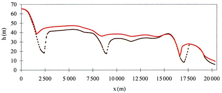
Preprints (www.preprints.org) | NOT PEER-REVIEWED | Posted: 31 July 2020 doi:10.20944/preprints202007.0753.v1

 technology are not always observed; on the other hand, as the following examples show, theoretical
 knowledge and support for physical modelling are not always sufficient. Experience and common
 sense are essential factors that need to be considered.

 3.1. Use of Software as a ‘Black Box’
 The most common formulations of the water quality process consist of systems of differential
 equations resulting from the mass conservation of a group of substances that are considered the most
 significant for the water quality process; however, the mathematical formulations developed for
 water quality process modelling are not consensual, since drastic simplifications are used as there are
 no universal laws for the reactions of water quality indicators [48].
 These equations depend on several coefficients/parameters that need to be specified a priori.
 These coefficients are site-dependent and depend also on the water’s characteristics. Thus, the
 establishment of mathematical formulations to characterize water quality processes (reactions)
 should always be questioned.
 To account for the lack of sufficient local information, water quality models are often used with
 coefficients obtained and validated by default, possibly in very different conditions.

 3.2. Imperfect Knowledge of Flow Interactions with the Bottom and Boundaries (Roughness Effects)
 This is a big problem, especially in the field of fluid mechanics. The dynamics of the water flow
 over irregular bottoms and boundaries with different characteristics and roughness, which normally
 are difficult to simulate with sufficient accuracy, translates into spurious data that can significantly
 affect the final results. The simulation of a real case shown below is proof enough of this. In terms of
 area A and flow Q, the Saint-Venant equations are written as
 
 + =0 (2)
 
 2 (ℎ + ) | | 
 + ( ) + + =0 (3)
 ⁄
 2 ℎ4 3
 where A is area, Q is flow, g is acceleration of gravity, ℎ is flow depth, represents bathymetry, ℎ
 is hydraulic radius and K is the Manning–Strickler coefficient.
 These equations were solved by the classic MacCormack method and applied to a hypothetical
 dam-break located upstream of Coimbra, Portugal. The objective was to evaluate the maximum wave
 height and wavefront arrival time at Penacova, a village located 20,325 m downstream of the Aguieira
 dam. Upstream of the dam, the reservoir was included up to a section located 21,000 m upstream.
 The Aguieira dam-break was therefore an internal boundary condition, located approximately in the
 middle of the simulated domain.
 As an initial condition downstream of Aguieira, a flow of 175 m3/s was considered, close to the
 maximum bottom discharge capacity. It was assumed that the dam would break almost instantly
 when the flow started to overtop the dam, with an approximate height of 89 m.
 Two scenarios were simulated, corresponding to different values of the Manning–Strickler
 coefficient. Because this coefficient is estimated empirically, it is advisable to estimate values for the
 flow variables corresponding to two “extreme” situations, among which that coefficient should be
 located. Thus, a first scenario was analysed for a K coefficient of the Manning–Strickler formula
 corresponding to the existence of minimum friction, under river regime conditions, in the order of
 40–45 m1/3s−1; for the second scenario, a K coefficient corresponding to the existence of maximum
 friction was adopted, with magnitude orders of 15–20 m1/3s−1.
 The flow heights obtained for the two scenarios are compared in Figure 7, in the stretch between
 the Aguieira dam and Penacova, after 52.5 min of simulation. The upper curve (red line) corresponds
 to the maximum friction condition (K = 15–20 m1/3s−1). Figure 8 shows the wavefront arrival times in
 both scenarios.

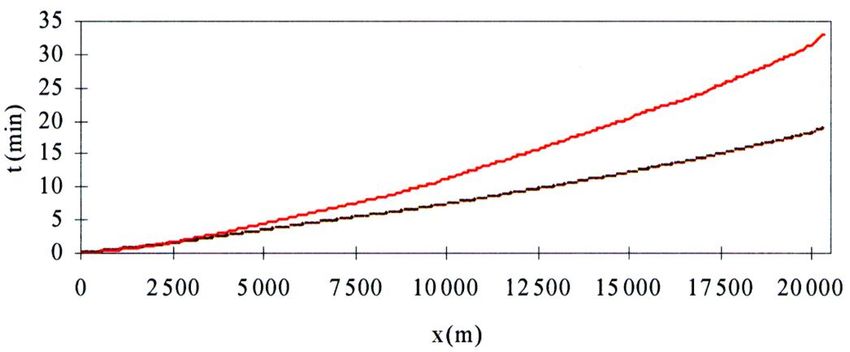
Preprints (www.preprints.org) | NOT PEER-REVIEWED | Posted: 31 July 2020 doi:10.20944/preprints202007.0753.v1

 Figure 7. Flow heights obtained for two scenarios of the Manning–Strickler coefficient;
 numerical solution obtained for K = 15–20 m1/3s−1 (red line) and for K = 40–45 m1/3s−1 (black line).

 Figure 8. Wavefront arrival times obtained for two scenarios of the Manning–Strickler coefficient;
 numerical solution obtained for K = 15–20 m1/3s−1 (red line) and for K = 40–45 m1/3s−1 (black line).

 3.3. Poor Formulation of the Initial and Boundary Conditions
 The initial conditions can be resting conditions, steady conditions (current) or unsteady
 conditions (waves or waves and currents), including possible interactions between different
 parameters. Different types of boundary conditions can be implemented: Dirichlet, Newmann and
 Hybrid schemes. Often, due to missing local information or implementation difficulties, the most
 appropriate initial and boundary conditions are not always implemented.

 3.4. Inadequate Mathematical Formulation for the Reproduction of the Physical Phenomenon
 By the end of the 1970s, models based on the Saint-Venant equations were frequently used in
 practical applications; however, in shallow water conditions and for some types of waves, models
 based on a non-dispersive theory, of which the Saint-Venant model is an example, are limited and
 are not usually able to compute satisfactory results over long periods of analysis (see [8] for a
 demonstration).
 Nowadays, it is generally accepted that for practical applications, the combined gravity wave
 effects in shallow water conditions must be considered. In addition, the refraction and diffraction
 processes, the swelling, reflection and breaking waves, all have to be considered.
 As Carmo [8] also states, several factors have made it possible to employ increasingly complex
 mathematical models. Not only has our theoretical knowledge of the phenomena involved improved
 greatly, but numerical methods have also been used more efficiently. The great advances made in
 computer technology, especially since the 1980s, improving information processing and enabling
 large amounts of data to be stored, have made it possible to use mathematical models of greater
 complexity and with fewer restrictions.

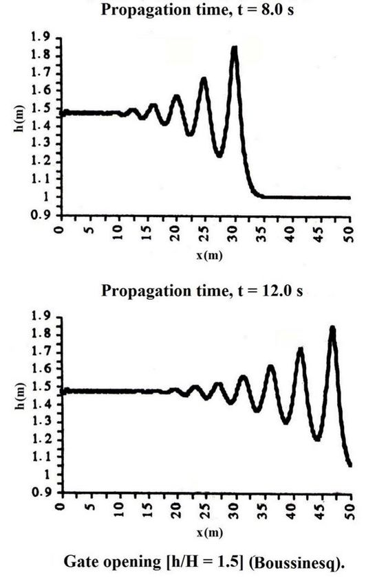
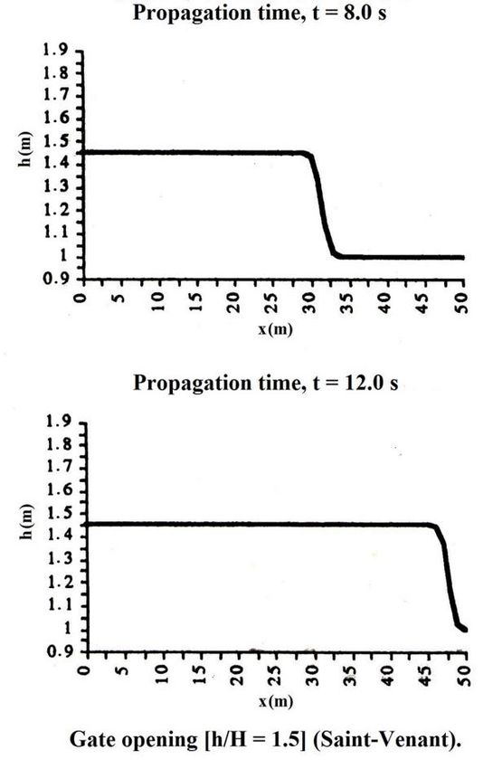
Preprints (www.preprints.org) | NOT PEER-REVIEWED | Posted: 31 July 2020 doi:10.20944/preprints202007.0753.v1

 As the following example shows, however advanced the mathematical models may be, it is
 advisable to always perform a prior analysis of the physical phenomena that are intended to be
 reproduced. To simulate a dam-break, the following question arises: what is the most suitable
 mathematical model for this purpose?
 To reproduce this phenomenon, two numerical models were tested: The Saint-Venant model
 (Equations (2) and (3) above) and the standard Boussinesq model shown below (Equations (4) and
 (5)).

 ℎ + ( ℎ) = 0 (4)

 1 1
 + + (ℎ + ) − ℎ [(ℎ ) ] + ℎ2 [( ) ] + ⁄( ℎ) = 0 (5)
 2 6
 where u is depth-averaged velocity, is fluid density and represents friction stresses at bottom.
 As in the Saint-Venant model (momentum Equation (2)), the Manning–Strickler approach was
 considered to compute the friction term (last term of Equation (4)). Figure 9 shows the same example
 of a dam break simulated by two different mathematical models (Saint-Venant and Boussinesq
 standard).

 Figure 9. Dam-break simulated by two different mathematical models: Saint-Venant on left and
 Boussinesq standard on right.

 The results shown in Figure 9 are located in the transition zone 0.40–0.55 of the ratio h/H, where
 h and H are initial depths downstream and upstream of the dam, respectively, as defined by [49]. In
 the transition zone, the undular surge front may begin to break, as predicted by the Saint-Venant
 equations, and it always breaks for the ratio h/H < 0.40, or the surge travelling downstream may be
 undular, as predicted by Boussinesq, as for h/H > 0.55.

Preprints (www.preprints.org) | NOT PEER-REVIEWED | Posted: 31 July 2020 doi:10.20944/preprints202007.0753.v1

 The different behaviours depend on various factors, such as friction, slope, dam-break type and
 dam-break time. This means that neither the Saint-Venant nor the Boussinesq equations can be used
 (as they are) to predict dam-break waves for an arbitrary value of the ratio r = h/H. A partial breaking
 for r = 0.515 is reported in [50].
 A comparison of the standard Serre model with a set of extended Serre equations was developed
 in [51]. As the classical Serre equations are only valid for shallow waters, we extended this model,
 with improved dispersive characteristics, for applications in intermediate water depths and quasi-
 deep waters [51,52].
 A comparison of experimental results with both the standard and improved/extended Serre
 models is detailed in [52]. Laboratory results were obtained in a flume 0.80 m wide with a submerged
 trapezoidal bar with slopes 1:10 (upstream) and 1:20 (downstream). Before and after the bar, the
 water depth was 0.40 m, with a reduction to 0.10 m above the bar.
 In [8,52], experimental and numerical results show that as the wave shoals up the front face and
 over the bar, in very shallow water conditions, it steepens dramatically, accumulating higher
 harmonics which are released on the downslope, producing an irregular pattern behind the bar. It is
 precisely these higher harmonics released behind the submerged structure that are not well simulated
 by the standard Serre equations. A complete set of Serre-type equations is written [51]:

 ℎ + ( ℎ) = 0 (6)

 ℎ2
 + + (ℎ + ) + (1 + )( − ℎℎ ) − (1 + ) + (ℎ + ) 
 3 
 ℎ2
 − ℎℎ (ℎ + ) − (ℎ + ) − ℎℎ 
 3 (7)
 ℎ2
 + ( − ) + ℎ( )2 (ℎ + ) + 2 (ℎ + ) 
 3
 ℎ
 + ( + ℎ ) + 2 + ⁄( ℎ) = 0
 2
 where ( ) = ℎ + 0.5ℎ + ( )2 .
 When = = 0, Serre standard equations are recovered, and with = 0.1308 and = 0.20,
 a set of extended Serre equations with improved dispersive characteristics is obtained.
 Figure 10 shows a comparison of the numerical results of the classical Serre model with the new
 set of extended Serre equations [8,52]. Globally, the numerical results of the improved Serre model
 agree quite well with the measured data.

 Figure 10. Comparison of experimental data with numerical results from Serre standard and Serre
 extended/improved.

 The influence of additional terms of dispersive origin included in the extended Serre equations
 is clearly shown in Figure 10. The classical Serre model results (dashed line) are clearly of lesser
 quality (see [50], Figures 17 and 20). This example highlights, once again, the need to make a prior
 analysis of the physical phenomena that are intended to be reproduced before using a numerical
 model.

Preprints (www.preprints.org) | NOT PEER-REVIEWED | Posted: 31 July 2020 doi:10.20944/preprints202007.0753.v1

 3.5. Inefficient Numerical Formulation, or Its Implementation, to Solve the Mathematical Model
 The use of a given numerical method depends on the type of equations to be solved and on how
 the numerical method was implemented. In a scientific article, it is insufficient to simply state that
 “Method X was used”. Variations in the implementation of “Method X” affect performance measures
 by factors of 2, 10 or more.
 In physics, there are three types of partial differential equations: elliptic equations, such as
 Laplace and Poisson, which represent or describe the potential of force fields in a variety of physical
 contexts; parabolic equations, which model diffusion or heat conduction problems; hyperbolic
 equations, which model wave motion.
 To solve elliptic equations, finite-difference methods are the simplest and most intuitive to
 implement; however, they are not the most efficient. The accuracy of Galerkin and least-squares
 methods is usually better, although the extra cost can negate this advantage for most problems. A
 current method of approximate solution of boundary value problems for elliptic partial differential
 equations is the method of boundary elements.
 For parabolic equations, a variety of methods are commonly used. Among them are: Finite
 difference schemes, Lax–Friedrichs and Lax–Wendroff, which can be viewed as modifications of
 forward-time central-space and a variety of Crank–Nicolson methods. Upwind schemes are also
 commonly used.
 For hyperbolic equations, many methods are also used, including: Finite difference schemes,
 first order and higher order of finite volume schemes; however, the finite element method is more
 common today and mathematically more efficient than the previous methods.
 In any of the methods or schemes, the analysis/proof of the concept of consistency is essential,
 which, together with stability, must imply the convergence of the numerical solution to the true
 solution.

 4. Discussion
 Analyses of river hydraulics, coastal hydraulics and water quality often require applications of
 heuristics and empirical experience. Usually, these analyses are performed through some
 simplification and modelling techniques, according to the experience of experts; however, the
 accuracy of the predictions depends largely on the numerical schemes, boundary conditions and
 model parameters. Adopting a numerical model suitable for a practical problem in a river or a coastal
 area is a complicated task that is not always successful. These predictive tools inevitably involve
 certain assumptions and/or limitations and should be applied only by experienced engineers who
 have a sufficiently comprehensive understanding of the problem.
 The numerical simulation of the Aguieira dam-break (Figures 7 and 8) showed significant
 differences in the maximum wave heights and in the arrival times of the wavefront about 20 km
 downstream. These differences were due exclusively to the friction term in the equations, which
 depends on a parameter that is difficult to quantify, even for experts.
 From the engineering point of view, the recommended methodology is to simulate with the
 maximum values (or an average of the maximum values) of friction (minimum K coefficient) to obtain
 the maximum wave heights along the valley and a second simulation with the minimum values (or
 an average of the minimum values) of the friction to obtain the arrival times of the wavefront. In this
 way, the estimates are guaranteed with security, which is essential for both people and goods.
 The physical simulation of a dam-break in a rectangular channel (Figure 9), under ideal
 conditions, shows that the wave patterns depend on the downstream to upstream water depth ratio.
 The numerical simulation shows that we need to use different mathematical models to describe the
 wave patterns generated as a function of the ratio values. The mathematical formulation to be used
 in the numerical simulation of a dam-break is thus a consequence of the learning acquired through
 physical modelling.
 The case of waves that propagate under certain conditions, such as those shown in Figure 10,
 proves the need for a careful assessment of the capabilities of a mathematical/numerical model to
 simulate the processes and phenomena involved with sufficient accuracy.

Preprints (www.preprints.org) | NOT PEER-REVIEWED | Posted: 31 July 2020 doi:10.20944/preprints202007.0753.v1

 In terms of recommendation, decision-making should not be based solely on the results of
 numerical modelling, unless decision-makers are convinced that the model is reliable for the problem
 at hand. Otherwise, a combination of four different factors must be used:
 • Numerical simulation;
 • Inspection and measurements;
 • Scale modelling;
 • Expertise.

 5. Conclusions
 To design a hydraulic system of significant dimensions, impact and costs, one or more of the
 following approaches are generally used:
 • Results of previous experimental studies and data measured in similar systems;
 • Physical modelling, using spatial scales sometimes too small and often distorted;
 • Computational models that solve increasingly complex mathematical formulations.
 Despite the significant improvement of computational models in recent decades, and
 subsequently, the improvement and widespread adoption of numerical methods, for many real-
 world problems, there are no mathematical and numerical solutions powerful enough to dispense
 the first two approaches. Likewise, physical modelling alone does not solve many real-world
 problems either. As experience has shown, instead of alternatives, physical and numerical models
 should be seen as complementary approaches.
 The need to maintain a strong investment in physical modelling is highlighted, together with
 the growth of numerical modelling and computational means, both to support the technical and
 scientific communities and to design and carry out projects that have significant impacts and costs.

 Funding: This research received no external funding.

 Conflicts of Interest: The author declares no conflict of interest.

 References
 1. Hinze, J.O. Turbulence, 2nd ed.; McGraw-Hill: New York, NY, USA, 1975.
 2. Rodi, W. Turbulence Models and Their Applications in Hydraulics: A State of the Art Review; IAHR: Delft, The
 Netherlands, 1980.
 3. Harry, M.; Zhang, H.; Lemckert, C.; Colleter, G. Measurement of the Scale Effect on Breaking Waves. In
 Proceedings of the Eleventh Pacific/Asia Offshore Mechanics Symposium, Shanghai, China, 12–16 October
 2014.
 4. Gregoretti, C.; Maltauro, A.; Lanzoni, S. Laboratory Experiments on the Failure of Coarse Homogeneous
 Sediment Natural Dams on a Sloping Bed. J. Hydraul. Eng. 2010, 136, 868–879, doi:10.1061/(ASCE)HY.1943-
 7900.0000259.
 5. Scharnke, J.; Bunnik, T.; Düz, B.; Bandringa, H.; Hallmann, R.; Helder, J. Linking Experimental and
 Numerical Wave Modelling. J. Mar. Sci. Eng. 2020, 8, 26, doi:10.3390/jmse8030198.
 6. Demir, A.; Dincer, A.E.; Bozkus, Z.; Tijsseling, A.S. Numerical and experimental investigation of damping
 in a dam-break problem with fluid-structure interaction. J. Zhejiang Univ. Sci. A 2019, 20, 258–271,
 doi:10.1631/jzus.A1800520.
 7. Nguyen, H.T.; Ahn, J.; Park, S.W. Numerical and Physical Investigation of the Performance of Turbulence
 Modeling Schemes around a Scour Hole Downstream of a Fixed Bed Protection. Water 2018, 10, 103,
 doi:10.3390/w10020103.
 8. Antunes do Carmo, J.S. Nonlinear and dispersive wave effects in coastal processes. J. Integr. Coast. Zone
 Manag. 2016, 16, 343–355, doi:10.5894/rgci660.
 9. Antunes do Carmo, J.S.; Pinho, J.L.S.; Vieira, J.M.P. Oil Spills in Coastal Zones: Predicting Slick Transport
 and Weathering Processes. Open Ocean Eng. J. 2010, 3, 129–142, doi:10.2174/1874835x01003010129.
 10. Pinho, J.L.S.; Antunes do Carmo, J.S.; Vieira, J.M.P. Mathematical modelling of oil spills in the Atlantic
 Iberian coastal waters. In Coastal Environment V, Incorporating Oil Spill Studies; WIT Transactions on Ecology

Preprints (www.preprints.org) | NOT PEER-REVIEWED | Posted: 31 July 2020 doi:10.20944/preprints202007.0753.v1

 and the Environment, 1st ed.; Brebbia, C.A., Saval Perez, J.M., Andion, L.G., Eds.; WITPRESS:
 Southampton, UK, 2004; Volume 68, pp. 337–347.
 11. Ahrens, C.D.; Henson, R. Weather Forecasting. In Essentials of Meteorology: An Invitation to the Atmosphere,
 8th ed.; Ahrens, C.D., Henson, R., Eds.; Cengage Learning: Boston, MA, USA, 2016; Volume 1, pp. 242–270.
 12. Argyropoulos, C.D.; Markatos, N.C. Recent advances on the numerical modelling of turbulent flows. Appl.
 Math. Model. 2015, 39, 693–732, doi:10.1016/j.apm.2014.07.001.
 13. Wilson, D.; Iacovides, H.; Craft, T. Assessment of RANS Turbulence Model Performance in Tight Lattice
 LWR Fuel Subchannels. In Proceedings of the 11th International Symposium on Turbulence and Shear
 Flow Phenomena (TSFP11), Southampton, UK, 30 July–2 August 2019.
 14. Wang. W.Q.; Yan, Y. Fluid-Structure Interaction Analysis of Flexible Plate with Partitioned Coupling
 Method. Appl. Math. Model. 2010, 34, 3817–3830, doi:10.1016/j.apm.2010.03.022.
 15. Chen, H.; Christensen, E.D. Development of a numerical model for fluid-structure interaction analysis of
 flow through and around an aquaculture net cage. Ocean Eng. 2017, 142, 597–615,
 doi:10.1016/j.oceaneng.2017.07.033.
 16. Over VLIZ: Scaling Issues in Hydraulic Modelling. Available online:
 http://www.vliz.be/wiki/Scaling_Issues_in_Hydraulic_Modelling (accessed on July 16, 2020).
 17. Coastal Wiki: Scaling Issues in Hydraulic Modelling. Available online:
 http://www.coastalwiki.org/wiki/Scaling_Issues_in_Hydraulic_Modelling (accessed on July 16, 2020).
 18. Carreiras, J.; Antunes do Carmo, J.; Seabra-Santos, F. Settlement of vertical piles exposed to waves. Coast.
 Eng. 2003, 47, 355–365, doi:10.1016/S0378-3839(02)00142-4.
 19. Xiang, Q.; Wei, K.; Qiu, F.; Yao, C.; Li, Y. Experimental Study of Local Scour around Caissons under
 Unidirectional and Tidal Currents. Water 2020, 12, 18, doi:10.3390/w12030640.
 20. World Register of Introduced Marine Species: Scaling Issues in Hydraulic Modelling. Available online:
 http://www.marinespecies.org/introduced/wiki/Scaling_Issues_in_Hydraulic_Modelling (accessed on
 July 15, 2020).
 21. Gao, F.; Wang, H.; Wang, H. Comparison of different turbulence models in simulating unsteady flow.
 Procedia Eng. 2017, 205, 3970–3977, doi:10.1016/j.proeng.2017.09.856.
 22. Heller, V. Scale effects in physical hydraulic engineering models. J. Hydraul. Res. 2011, 49, 293–306,
 doi:10.1080/00221686.2011.578914.
 23. Briggs, M.J. Basics of Physical Modeling in Coastal and Hydraulic Engineering; ERDC/CHL CHETN-XIII-3; US
 Army Corps of Engineers: Washington, DC, USA, 2013; p. 11.
 24. Saidani, M.; Shibani, A. Use of Physical and Numerical Models in Engineering Design Education. In
 Proceedings of the International Conference on Industrial Engineering and Operations Management, Bali,
 Indonesia, 7–9 January 2014.
 25. Marques, J.C. Experimental modelling vs. numerical simulation in geotechnical training. In Proceedings of
 the IEEE Global Engineering Education Conference (EDUCON), Istanbul, Turkey, 3–5 April 2014; pp. 991–
 994. Available online: https://ieeexplore.ieee.org/document/6826222 (accessed on July 15, 2020).
 26. Chen, Z.; Chen, B. Recent Research and Applications of Numerical Simulation for Dynamic Response of
 Long-Span Bridges Subjected to Multiple Loads. Sci. World J. 2014, 2014, 17, doi:10.1155/2014/763810.
 27. Al-Janabi, A.M.S.; Ghazali, A.H.; Ghazaw, Y.M.; Afan, H.A.; Al-Ansari, N.; Yaseen, Z.M. Experimental and
 Numerical Analysis for Earth-Fill Dam Seepage. Sustainability 2020, 12, 2490, doi:10.3390/su12062490.
 28. Ninot, C.G.; Mendes, L.; Viseu, T.; Vicent, J.G.; Carrero, A.D.; González, J.O.; Domínguez, O.H.; Iglesias,
 F.R.; Gutiérrez, E.R. Experimental and Numerical Study of a Chute Spillway. In Proceedings of the Second
 International Dam World Conference, Lisbon, Portugal, 21–24 April 2015.
 29. Google: Longest Suspension Bridge in the World—Akashi Kaikyo Bridge. Available online:
 https://youtu.be/vH8cqgnvsEs (accessed on July 16, 2020).
 30. Augustyn. The Editors of Encyclopædia Britannica. Three Gorges Dam. 2020. Available online:
 https://www.britannica.com/topic/Three-Gorges-Dam (accessed on July 15, 2020).
 31. Google: The Complete Model of the Akashi Kaikyo Bridge and the Boundary Layer Wind Tunnel.
 Available online:
 https://www.researchgate.net/profile/Ibuki_Kusano/publication/281550286/figure/fig21/AS:645733061509
 130@1530966167268/2-The-complete-model-of-the-Akashi-Kaikyo-Bridge-and-the-boundary-layer-wind-
 tunnel.png (accessed on July 16, 2020).

Preprints (www.preprints.org) | NOT PEER-REVIEWED | Posted: 31 July 2020 doi:10.20944/preprints202007.0753.v1

 32. Google: The Physical Model of no. 3 Powerhouse-Dam Section of the Three-Gorges Dam. Available online:
 https://www.semanticscholar.org/paper/Stability-assessment-of-the-Three-Gorges-Dam-China%2C-Liu-
 Feng/895247023ba961db9d14c5fdf9542c22c487c601/figure/31 (accessed on July 16, 2020).
 33. Miyata, T.; Yamaguchi, K. Aerodynamics of wind effects on the Akashi Kaikyo Bridge. J. Wind Eng. Ind.
 Aerodyn. 1993, 48, 287–315, doi:10.1016/0167-6105(93)90142-B.
 34. Miyata, T.; Yamada, H.; Katsuchi, H.; Kitagawa, M. Full-scale measurement of Akashi–Kaikyo
 Bridgeduring typhoo. J. Wind Eng. Ind. Aerodyn. 2002, 90, 1517–1527, doi:10.1016/S0167-6105(02)00267-2.
 35. Diana, G.; Fiammenghi, G.; Belloli, M.; Rocchi, D. Wind tunnel tests and numerical approach for long span
 bridges: The Messina bridge. J. Wind Eng. Ind. Aerodyn. 2013, 122, 38–49, doi:10.1016/j.jweia.2013.07.012.
 36. Diana, G.; Rocchi, D.; Belloli, M. Wind tunnel: A fundamental tool for long-span bridge design. Struct.
 Infrastruct. Eng. 2015, 11, 533–555, doi:10.1080/15732479.2014.951860.
 37. Liu, J.; Feng, X.-T.; Ding, X.-L.; Zhang, J.; Yue, D.-M. Stability assessment of the Three-Gorges Dam
 foundation, China, using physical and numerical modeling—Part I: Physical model tests. Int. J. Rock Mech.
 Min. Sci. 2003, 40, 609–631, doi:10.1016/S1365-1609(03)00055-8.
 38. Liu, J.; Feng, X.-T.; Ding, X.-L. Stability assessment of the Three-Gorges Dam foundation, China, using
 physical and numerical modeling—Part II: Numerical modeling. Int. J. Rock Mech. Min. Sci. 2003, 40, 633–
 652, doi:10.1016/S1365-1609(03)00056-X.
 39. Jabbari, M.; Bulatova, R.; Hattel, J.H.; Bahl, C.R.H. An evaluation of interface capturing methods in a VOF
 based model for multiphase flow of a non-Newtonian ceramic in tape casting. Appl. Math. Model. 2014, 38,
 3222–3232.
 40. Deshande, S.S.; Trujillo, M.F.; Wu, X.; Chahine, G. Computational and experimental characterization of a
 liquid jet plunging into a quiescent pool at shallow inclination. Int. J. Heat Fluid Flow 2012, 34, 1–14,
 doi:10.1016/j.ijheatfluidflow.2012.01.011.
 41. Hirt, C.; Nichols, B. Volume of fluid method for the dynamics of free boundaries. J. Comput. Phys. 1981, 39,
 201–225, doi:10.1016/0021-9991(81)90145-5.
 42. Kang, S.; Sotiropoulos, F. Numerical study of flow dynamics around a stream restoration structure in a
 meandering channel. J. Hydraul. Res. 2015, 53, 178–185, doi:10.1080/00221686.2015.1023855.
 43. Duró. G.; Crosato, A.; Tassi, P. Numerical study on river bar response to spatial variations of channel width.
 Adv. Water Resour. 2016, 93, 21–38, doi:10.1016/j.advwatres.2015.10.003.
 44. Farsirotou, E.D.; Kotsopoulos, S.I. Free-Surface Flow Over River Bottom Sill: Experimental and Numerical
 Study. Environ. Process. 2015, 2, 133–139, doi:10.1007/s40710-015-0090-6.
 45. Mali, V.K.; Kuiry, S.N. Experimental and numerical study of flood in a river-network-floodplain set-up. J.
 Hydraul. Res. 2020, doi:10.1080/00221686.2019.1698471.
 46. Tsoukala, V.K.; Katsardi, V.; Hdjibiros, K.; Moutzouris, C.I. Beach Erosion and Consequential Impacts Due
 to the Presence of Harbours in Sandy Beaches in Greece and Cyprus. Environ. Process. 2015, 2, 55–71,
 doi:10.1007/s40710-015-0096-0.
 47. Antunes do Carmo, J.S. Coastal defences and engineering works. In Encyclopedia of the UN Sustainable
 Development Goals. Life Below Water 2020; Filho, W.L., Özuyar, P.G., Azul, A.M., Brandli, L.L., Wall, T., Eds.;
 Springer: Berlin/Heidelberg, Germany (accepted, in press).
 48. Pinho, J.L.S.; Vieira, J.M.P.; Antunes do Carmo, J.S. Hydroinformatic environment for coastal waters
 hydrodynamics and water quality modelling. Adv. Eng. Soft 2004, 35, 205–222,
 doi:10.1016/j.advengsoft.2004.01.001.
 49. Castro-Orgaz, O.; Hubert Chanson, H. Undular and broken surges in dam-break fows: A review of wave
 breaking strategies in a Boussinesq-type framework. Environ. Fluid Mech. 2020, doi:10.1007/s10652-020-
 09749-3.
 50. Antunes do Carmo, J.S.; Ferreira, J.A.; Luís Pinto, L. On the accurate simulation of nearshore and dam break
 problems involving dispersive breaking waves. Wave Motion 2019, 85, 125–143,
 doi:10.1016/j.wavemoti.2018.11.008.
 51. Antunes do Carmo, J.S. Boussinesq and Serre type models with improved linear dispersion characteristics:
 Applications. J. Hydraul. Res. 2013, 51, 719–727, doi:10.1080/00221686.2013.814090.
 52. Antunes do Carmo, J.S. Extended Serre Equations for Applications in Intermediate Water Depths. Open
 Ocean Eng. J. 2013, 6, 16–25, doi:10.2174/1874835×01306010016.