HIERARCHICAL AUTOREGRESSIVE MODELING FOR NEURAL VIDEO COMPRESSION
←
→
Page content transcription
If your browser does not render page correctly, please read the page content below

Under review as a conference paper at ICLR 2021

H IERARCHICAL AUTOREGRESSIVE M ODELING
FOR N EURAL V IDEO C OMPRESSION

 Anonymous authors
 Paper under double-blind review

                                            A BSTRACT
         Recent work by Marino et al. (2020) showed improved performance in sequential
         density estimation by combining masked autoregressive flows with hierarchical
         latent variable models. We draw a connection between such autoregressive gener-
         ative models and the task of lossy video compression. Specifically, we view recent
         neural video compression methods (Lu et al., 2019; Yang et al., 2020b; Agustsson
         et al., 2020) as instances of a generalized stochastic temporal autoregressive trans-
         form, and propose avenues for enhancement based on this insight. Comprehensive
         evaluations on large-scale video data show improved rate-distortion performance
         over both state-of-the-art neural and conventional video compression methods.

1   I NTRODUCTION
With recent advances, deep generative modeling has seen a surge in applications, including neural-
based compression. Generative models have already demonstrated empirical improvements in im-
age compression, outperforming classical codecs, such as BPG (Bellard, 2014). In contrast, the less
developed area of neural-based video compression remains challenging due to complex temporal
dependencies operating at multiple scales. Nevertheless, recent neural video codecs have shown
promising performance gains (Agustsson et al., 2020), in some cases on par with current hand-
designed, classical codecs, e.g., HEVC. Compared with hand-designed codecs, learnable codecs
can be tuned to specific data modalities, providing a promising approach for streaming specialized
content, such as sporting events or video chatting. Therefore, improving neural-based video com-
pression is a necessity for dealing with the ever-growing amount of video content being created.
Source compression fundamentally involves decorrelation, i.e., transforming input data into white
noise distributions that can be easily modeled and entropy-coded. Thus, improving a model’s ca-
pability to decorrelate data automatically improves its compression performance. Likewise, we can
improve the associated entropy model (i.e., the model’s prior) to capture any remaining dependen-
cies. Just as compression techniques attempt to remove structure, generative models attempt to
model structure. One family of models, autoregressive flows, maps between less structured distribu-
tions, e.g., uncorrelated noise, and more structured distributions, e.g., images or video (Dinh et al.,
2014; 2016). The inverse mapping can remove dependencies in the data, making it more amenable
for compression. Thus, a natural question to ask is how autoregressive flows can best be utilized in
compression, and if mechanisms in existing compression schemes can be interpreted as flows.
This paper draws on recent insights in hierarchical sequential latent variable models with autoregres-
sive flows (Marino et al., 2020). In particular, we identify connections between this family of models
and a recently proposed neural video codec based on scale-space warping (Agustsson et al., 2020).
By interpreting this technique as a specific instantiation of a flow, we propose various alternatives
and improvements, drawing on insights from generative modeling and autoregressive flows.
In more detail, our main contributions are as follows:

      1. A new framework. We interpret existing video compression methods through the more
         general framework of generative modeling, variational inference, and autoregressive flows,
         allowing us to readily investigate extensions and ablations. In particular, we compare fully
         data-driven approaches with motion-estimation-based neural compression schemes, and
         consider a more expressive prior model for better entropy coding (described in the second
         bullet point below). This framework also provides directions for future work.

                                                  1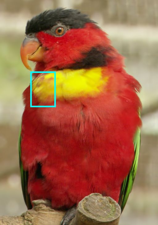
Under review as a conference paper at ICLR 2021

         2. A new model. Our main proposed model extends the Scale-Space Flow (SSF) (Agustsson
            et al., 2020) model. Following the classical predictive coding approach to video compres-
            sion, this model uses motion estimation to predict the frame being compressed, and further
            compresses the residual obtained by subtraction. We improve on SSF by:
               • Incorporating a learnable scaling transform, to allow for more expressive and accurate
                 reconstruction. Augmenting a shift transform by scale-then-shift is inspired by im-
                 provements from extending NICE (Dinh et al., 2014) to RealNVP (Dinh et al., 2016).
               • Introducing a structured prior over the two sets of latent variables in the probabilistic
                 generative model of SSF (based our generative framework), corresponding to jointly
                 encoding the motion information and residual information. As the two tend to be
                 spatially correlated, encoding residual information conditioned on motion information
                 results in a more informed prior model, and thus better entropy model, for the residual
                 information, cutting down its bit-rate that typically dominates the overall bit-rate.
         3. A new dataset. The neural video compression community is lacking large, high-resolution
            benchmark datasets. While we performed extensive experiments on the publicly avail-
            able Vimeo-90k dataset (Xue et al., 2019), we also collected and utilized a larger dataset,
            YouTube-NT1 , available through executable scripts. Since no training data was publicly re-
            leased for the previous state-of-the-art method (Agustsson et al., 2020), YouTube-NT will
            be a useful resource for making and comparing further progress in this field.

2       R ELATED W ORK
We divide relevant related work into three categories: neural image compression, neural video com-
pression, and sequential generative models.

Neural Image Compression. Considerable progress has been made by applying neural networks
to image compression. Early works proposed by Toderici et al. (2017) and Johnston et al. (2018)
leveraged LSTMs to model spatial correlations of the pixels within an image. Theis et al. (2017) first
proposed an autoencoder architecture for image compression and used the straight-through estima-
tor (Bengio et al., 2013) for learning a discrete latent representation. The connection to probabilistic
generative models was drawn by Ballé et al. (2017), who firstly applied variational autoencoders
(VAEs) (Kingma & Welling, 2013) to image compression. In subsequent work, Ballé et al. (2018)
encoded images with a two-level VAE architecture involving a scale hyper-prior, which can be fur-
ther improved by autoregressive structures (Minnen et al., 2018; Minnen & Singh, 2020) or by
optimization at encoding time (Yang et al., 2020d). Yang et al. (2020e) and Flamich et al. (2019)
demonstrated competitive image compression performance without a pre-defined quantization grid.

Neural Video Compression. Compared to image compression, video compression is a signifi-
cantly more challenging problem, as statistical redundancies exist not only within each video frame
(exploited by intra-frame compression) but also along the temporal dimension. Early works by Wu
et al. (2018); Djelouah et al. (2019) and Han et al. (2019) performed video compression by predict-
ing future frames using a recurrent neural network, whereas Chen et al. (2019) and Chen et al. (2017)
used convolutional architectures within a traditional block-based motion estimation approach. These
early approaches did not outperform the traditional H.264 codec and barely surpassed the MPEG-2
codec. Lu et al. (2019) adopted a hybrid architecture that combined a pre-trained Flownet (Dosovit-
skiy et al., 2015) and residual compression, which leads to an elaborate training scheme. Habibian
et al. (2019) and Liu et al. (2019) combined 3D convolutions for dimensionality reduction with ex-
pressive autoregressive priors for better entropy modeling at the expense of parallelism and runtime
efficiency. Our method extends a low-latency model proposed by Agustsson et al. (2020), which
allows for end-to-end training, efficient online encoding and decoding, and parallelism.

Sequential Deep Generative Models. We drew inspiration from a body of work on sequential
generative modeling. Early deep learning architectures for dynamics forecasting involved RNNs
(Chung et al., 2015). Denton & Fergus (2018) and Babaeizadeh et al. (2017) used VAE-based
stochastic models in conjunction with LSTMs to model dynamics. Li & Mandt (2018) introduced
    1
        https://anonymous.4open.science/r/7fba4f65-e003-446e-81d5-fdd5fed01335/

                                                     2
Under review as a conference paper at ICLR 2021

both local and global latent variables for learning disentangled representations in videos. Other
video generation models used generative adversarial networks (GANs) (Vondrick et al., 2016; Lee
et al., 2018) or autoregressive models and normalizing flows (Rezende & Mohamed, 2015; Dinh
et al., 2014; 2016; Kingma & Dhariwal, 2018; Kingma et al., 2016; Papamakarios et al., 2017).
Recently, Marino et al. (2020) proposed to combine latent variable models with autoregressive flows
for modeling dynamics at different levels of abstraction, which inspired our models and viewpoints.

3     V IDEO C OMPRESSION THROUGH D EEP AUTOREGRESSIVE M ODELING
We identify commonalities between hierarchical autoregressive flow models (Marino et al., 2020)
and state-of-the-art neural video compression architectures (Agustsson et al., 2020), and will use
this viewpoint to propose improvements on existing models.

3.1   BACKGROUND

We first review VAE-based compression schemes (Ballé et al., 2017; Theis et al., 2017) and formu-
late existing low-latency video codecs in this framework. We also review flow-based models.

Generative Modeling and Source Compression. Let x1:T ∈ RT ×D be a sequence of video
frames. Lossy compression seeks to find the shortest description R of x1:T without exceeding
a certain level of information loss D. The distortion D measures how much reconstruction error
accrues due to encoding x1:T into a latent representation z̄1:T and subsequently decoding it back to
x̂1:T , while R measures the bit rate (file size). In learned compression methods (Ballé et al., 2017;
Theis et al., 2017), the above process is parameterized by flexible functions f (“encoder”) and g
(“decoder”) that map between the input video and its latent representation z̄1:T = f (x1:T ). Using a
parameter β, both terms can be weighted against each other:
                               L = D(x1:T , g(bz̄1:T e)) + βR(bz̄1:T e).
We adopt the end-to-end compression approach of Ballé et al. (2017); Han et al. (2019), which
approximates the rounding operations (b•e) by uniform noise injection to enable gradient-based
optimization during training. With an appropriate choice of probability model p(z1:T ), the approxi-
mated version of the above R-D objective then corresponds to the VAE objective:
                        L̃ = Eq(z1:T |x1:T ) [− log p(x1:T |z1:T ) − log p(z1:T )].                   (1)
In this model, the likelihood p(x1:T |z1:T ) follows a Gaussian distribution with mean x̂1:T = g(z1:T )
                             β
and diagonal covariance 2 log   2 I, the approximate posterior q is chosen to be a unit-width uniform
(thus zero-differential-entropy) distribution whose mean z̄1:T is predicted by an amortized inference
network f . The prior density p(z1:T ) interpolates its discretized version, so that it measures the code
length of discretized z̄1:T after entropy-coding.

Low-Latency Sequential Compression We specialize Eq. 1 to make it suitable for low-latency
video compression, widely used in both conventional and recent neural codecs (Rippel et al., 2019;
Agustsson et al., 2020). To this end, we encode and decode individual frames xt in sequence.
Given the ground truth current frame xt and the previously reconstructed frames x̂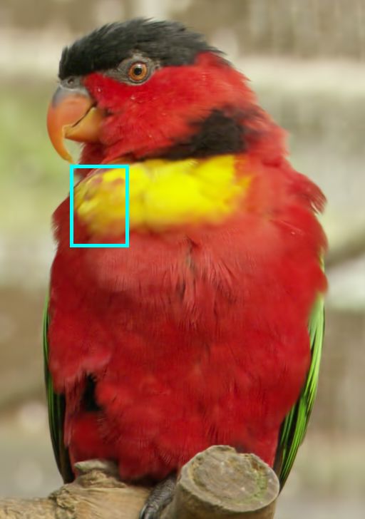
Under review as a conference paper at ICLR 2021

in terms of a simpler distribution of its underlying noise variables y1:T through the following au-
toregressive transform and its inverse:
                                                                       xt −hµ (x
Under review as a conference paper at ICLR 2021
(a) (b) (c)
split split
Figure 1: Model Diagrams. Graphical models for the generative and inference procedures of current
frame xt , for various neural video compression methods. Random variables are shown in circles,
all other quantities are deterministically computed; solid and dashed arrows describe computational
dependency during generation (decoding) and inference (encoding), respectively. Purple nodes cor-
respond to neural encoders (CNNs) and decoders (DNNs), and green nodes implement temporal
autoregressive transform. (a) TAT; (b) SSF; (c) STAT or STAT-SSF; the magenta box highlights the
additional proposed scale transform absent in SSF, and red arrow from wt to vt shows the proposed
(optional) structured prior. See Fig. 7 in appendix for computational diagram of the structured prior.
β
adds additional white noise to x̂, with x := x̂ + , ∼ N (0, 2 log 2 I). Thus, the generative process
from y to x is no longer an autoregressive flow. Regardless, TAT was shown to better capture the
low-level dynamics of video frames than the autoencoder (fz , gz ) alone, and the inverse transform
decorrelates raw video frames to simplify the input to the encoder fz (Yang et al., 2020b).
DVC (Lu et al., 2019) and Scale-Space Flow (SSF, Agustsson et al. (2020)). The second class
of models captured by Eq. 3 belong to the conventional video compression framework based on
predictive coding (Cutler, 1952; Wiegand et al., 2003; Sullivan et al., 2012); both models make use
of two sets of latent variables z1:T = {w1:T , v1:T } to capture different aspects of information being
compressed, where w captures estimated motion information used in warping prediction, and v
helps capture residual error not predicted by warping.
Like most classical approaches to video compression by predictive coding, the reconstruction trans-
form in the above models has the form of a prediction shifted by residual error (decoded noise), and
lacks the scaling factor hσ compared to the autoregressive transform in Eq. 3
x̂t = hwarp (x̂t−1 , gw (wt )) + gv (vt , wt ). (5)
Above, gw and gv are DNNs, ot := gw (wt ) has the interpretation of an estimated optical flow (mo-
tion) field, hwarp is the computer vision technique of warping, and the residual rt := gv (vt , wt ) =
x̂t − hwarp (x̂t−1 , ot ) represents the prediction error unaccounted for by warping. Lu et al. (2019)
only makes use of vt in the residual decoder gv , and performs simple 2D warping by bi-linear inter-
pretation; SSF (Agustsson et al., 2020) augments the optical flow (motion) field ot with an additional
scale field, and applies scale-space-warping to the progressively blurred versions of x̂t−1 to allow
for uncertainty in the warping prediction. The encoding procedure in the above models compute
the variational mean parameters as w̄t = fw (xt , x̂t−1 ), v̄t = fv (xt − hwarp (x̂t−1 , gw (wt ))), cor-
responding to a structured posterior q(zt |xt , zUnder review as a conference paper at ICLR 2021
Previous reconstruction x̂t−1 Magnitude of the proposed scale Rate savings in residual encoding bv̄te Rate savings in residual encoding bv̄te
by STAT-SSF-SP parameter σ̂t = hσ (x̂t−1, bw̄te) relative to STAT-SSF (BPP=0.053) relative to SSF (BPP=0.075)
0.4 100 100
50 50
0.2 0 0
−50 −50
0.0 −100 −100
SSF warping (mean) prediction Current reconstruction x̂t = µ̂t + r̂t
µ̂t = hµ(x̂t−1, bw̄te) Decoded noise ŷt = gv (bv̄te, bw̄te) Decoded residual r̂t = ŷt σ̂t by STAT-SSF-SP (BPP=0.046)
Figure 2: Visualizing the proposed STAT-SSF-SP model on one frame of UVG video “Shak-
eNDry”. Two methods in comparison, STAT-SSF (proposed) and SSF (Agustsson et al., 2020), have
comparable reconstruction quality to STAT-SSF-SP but higher bit-rate; the (BPP, PSNR) for STAT-
SSF-SP, STAT-SSF, and SSF are (0.046, 36.97), (0.053, 36.94), and (0.075, 36.97), respectively. In
this example, the warping prediction µ̂t = hµ (x̂t−1 , bw̄t e) incurs large error around the dog’s mov-
ing contour, but models the mostly static background well, with the residual latents bv̄t e taking up
an order of magnitude higher bit-rate than bw̄t e in the three methods. The proposed scale parameter
σ̂t gives the model extra flexibility when combining the noise ŷt (decoded from (bv̄t e, bw̄t e)) with
the warping prediction µ̂t (decoded from bw̄t e only) to form the reconstruction x̂t = µ̂t + σ̂t ŷt :
the scale σ̂t downweights contribution from the noise ŷt in the foreground where it is very costly,
and reduces the residual bit-rate R(bv̄t e) (and thus the overall bit-rate) compared to STAT-SSF and
SSF (with similar reconstruction quality), as illustrated in the third and fourth figures in the top row.
seen as an extended version of the SSF model, whose shift transform hµ is preceded by a new
learned scale transform hσ .
Structured Prior (SP). Besides improving the autoregressive transform (affecting the likelihood
model for xt ), one variant of our approach also improves the topmost generative hierarchy in the
form of a more expressive latent prior p(z1:T ), affecting the entropy model for compression. We ob-
serve that motion information encoded in wt can often be informative of the residual error encoded
in vt . In other words, large residual errors vt incurred by the mean prediction hµ (x̂t−1 , wt ) (e.g., the
result of warping the previous frame hµ (x̂t−1 )) are often spatially collocated with (unpredictable)
motion as encoded by wt . The original SSF model’s prior factorizes as p(wt , vt ) = p(wt )p(vt )
and does not capture such correlation. We therefore propose a structured prior by introducing condi-
tional dependence between wt and vt , so that p(wt , vt ) = p(wt )p(vt |wt ). At a high level, this can
be implemented by introducing a new neural network that maps wt to parameters of a parametric
distribution of p(vt |wt ) (e.g., mean and variance of a diagonal Gaussian distribution). This results
in variants of the above models, STAT-SP and STAT-SSF-SP, where the structured prior is applied
on top of the proposed STAT and STAT-SSF models.
4 E XPERIMENTS
In this section, we train our models both on existing dataset as well as our new YouTube-NT dataset,
and improve over state-of-the-art neural as well as classical video compression methods when evalu-
ating on several publically available benchmark datasets. Lower-level modules and training scheme
for our models largely follow Agustsson et al. (2020); we provide detailed model diagrams and
schematic implementation, including the proposed scaling transform and structured prior, in Ap-
pendix A.4. We also implement a more computationally efficient version of scale-space warping
(Agustsson et al., 2020) based on Gaussian pyramid and interpolation (instead of naive Gaussian
blurring); pseudocode is available at Appendix A.3.
4.1 T RAINING DATASETS
Vimeo-90k (Xue et al., 2019) consists of 90,000 clips of 7 frames at 448x256 resolution collected
from vimeo.com. As this dataset has been used in previous works (Lu et al., 2019; Yang et al.,
2020a; Liu et al., 2019), it provides a benchmark for comparing models. While other publicly-
6Under review as a conference paper at ICLR 2021
available video datasets exist, e.g., Kinetics (Carreira & Zisserman, 2017), such datasets are lower-
resolution and primarily intended for human action recognition. Accordingly, previous works that
have trained using Kinetics generally report sub-par PSNR-bitrate performance (Wu et al., 2018;
Habibian et al., 2019; Golinski et al., 2020). Agustsson et al. (2020) uses a significantly larger and
higher-resolution dataset collected from youtube.com, however, this is not publicly available.
YouTube-NT. This is our new dataset. We collected 8,000 nature videos and movie/video-game
trailers from youtube.com and processed them into 300k high-resolution (720p) clips, which we
refer to as YouTube-NT. In contrast to existing datasets (Carreira & Zisserman, 2017; Xue et al.,
2019), we provide YouTube-NT in the form of customizable scripts to enable future compression
research. Table 1 compares the current version of YouTube-NT with Vimeo-90k (Xue et al., 2019)
and with Google’s proprietary training dataset (Agustsson et al., 2020). In Figure 5b, we display the
evaluation performance of the SSF model architecture after training on each dataset.
Table 1: Overview of Training Datasets.
Dataset name Clip length Resolution # of clips # of videos Public Configurable
–
Vimeo-90k 7 frames 448x256 90,000 5,000 3 X
YouTube-NT (ours) 6-10 frames 1280x720 300,000 8,000 3 3
Agustsson 2020 et al. 60 frames 1280x720 700,000 700,000 7 7
4.2 T RAINING AND E VALUATION S CHEME
Training. All models are trained with three consecutive frames and batchsize 8, which are randomly
selected from each clip, then randomly cropped to 256x256. We trained on MSE loss, following
similar procedure to Agustsson et al. (2020) (Refer to Appendix A.2 for details).
Evaluation. We evaluate compression performance on the widely used UVG (Mercat et al., 2020)
and MCL JCV (Wang et al., 2016) test datasets, which both consist of raw videos in YUV420
format. UVG is widely used for testing the HEVC codec and contains seven 1080p videos at 120fps
with smooth and mild motions or stable camera moving. MCL JCV contains thirty 1080p videos
at 30fps, which are generally more diverse, with a higher degree of motion and a more unstable
camera.
We compute the bit rate (bits-per-pixel, BPP) and the reconstruction quality as measured in PSNR,
averaged across all frames. We note that PSNR is a more challenging metric than MS-SSIM (Wang
et al., 2003) for learned codecs (Lu et al., 2019; Agustsson et al., 2020; Habibian et al., 2019;
Yang et al., 2020a;c). Since existing neural compress methods assume video input in RGB format
(24bits/pixel), we follow this convention in our evaluations for meaningful comparisons. We note
that HEVC also has special support for YUV420 (12bits/pixel), allowing it to exploit this more
compact file format and effectively halve the input bitrate on our test videos (which were coded
in YUV420 by default), giving it an advantage over all neural methods. Regardless, we report the
performance of HEVC in YUV420 mode (in addition to the default RGB mode) for reference.
Table 2: Overview of models and codecs.
Model Name Category Vimeo-90k Youtube-NT Remark
STAT-SSF Proposed 3 3 Proposed autoregressive transform with efficient scale-space flow model
STAT-SSF-SP Proposed 3 7 Proposed autoregressive transform with efficient scale-space flow model and structured prior
SSF Baseline 3 3 Agustsson et al. 2020 CVPR
DVC Baseline 3 7 Lu et al. 2019 CVPR
VCII Baseline 7 7 Wu et al. 2018 ECCV (Trained on Kinectics dataset (Carreira & Zisserman, 2017))
DGVC Baseline 3 7 Han et al. 2019 NeurIPS without using future frames
TAT Baseline 3 7 Yang et al. 2020b ICML Workshop
HEVC Baseline N/A N/A State-of-the-art conventional codec with RGB color space input
HEVC(YUV) Baseline N/A N/A State-of-the-art conventional codec with YUV 4:2:0 color space input
STAT Ablation 3 3 Replace scale space flow in STAT-SSF with neural network
SSF-SP Ablation 7 3 Scale space flow model with structured prior
4.3 BASELINE A NALYSIS
We trained our models on Vimeo-90k data, in order to compare with published results of baseline
models listed in Table 2. Figure 3a compares our proposed models (STAT-SSF, STAT-SSF-SP) with
7Under review as a conference paper at ICLR 2021
UVG MCL_JCV
40
40
39
39
38 38
HEVC(YUV420)
PSNR(dB)
PSNR(dB)
37 37
HEVC
DVC(Lu et al. 2019) HEVC(YUV420)
36 VCII(Wu et al. 2018) 36 HEVC
SSF(Agustsson et al. 2020) SSF(Agustsson et al. 2020)
STAT-SSF(Proposed) 35 STAT-SSF(Proposed)
35 STAT-SSF-SP(Proposed) STAT-SSF-SP(Proposed)
STAT(Ablation) STAT(Ablation)
DGVC(Han et al. 2019) 34 TAT(Yang et al. 2020b)
34 TAT(Yang et al. 2020b) DGVC(Han et al. 2019)
33
0.00 0.05 0.10 0.15 0.20 0.25 0.30 0.35 0.40 0.45 0.0 0.1 0.2 0.3 0.4 0.5
Bits/Pixel Bits/Pixel
(a) (b)
Figure 3: Rate-Distortion Performance of various models and ablations. Results are evaluated on
(a) UVG and (b) MCL JCV datasets. All the neural-based models (except VCII (Wu et al., 2018))
are trained on Vimeo-90k. STAT-SSF-SP (proposed) achieves the best performance.
(a) HEVC; (b) SSF; (c) STAT-SSF (ours); (d) STAT-SSF-SP (ours);
BPP = 0.087, BPP = 0.082, BPP = 0.0768, BPP = 0.0551,
PSNR = 38.099 PSNR = 37.440 PSNR = 38.108 PSNR = 38.097
Figure 4: Qualitative comparisons of various methods on a frame from MCL-JCV video 30. Fig-
ures in the bottom row focus on the same image patch on top. Here, models with the proposed
scale transform (STAT-SSF and STAT-SSF-SP) outperform the ones without, yielding visually more
detailed reconstructions at lower rates; structured prior (STAT-SSF-SP) reduces the bit-rate further.
previous state-of-the-art classical codec HEVC and neural codecs on the UVG evaluation dataset.
Our STAT-SSF-SP model provides superior performance at bitrates ≥ 0.07 BPP, outperforming
conventional HEVC even in its favored YUV 420 mode and state-of-the-art neural method SSF
8Under review as a conference paper at ICLR 2021
(a) (b)
Figure 5: Ablations & Comparisons. (a) An ablation study on our proposed components. (b)
Performance of SSF (Agustsson et al., 2020) trained on different datasets. Both sets of results are
evaluated on UVG.
(Agustsson et al., 2020) , as well as the established DVC (Lu et al., 2019), which leverages a more
complicated model and multi-stage training procedure. We also note that, as expected, our proposed
STAT model improves over TAT (Yang et al., 2020b), with the latter lacking stochasticity in the
autoregressive transform compared to our proposed STAT and its variants.
Figure 3a shows that the performance ranking on MCL JCV is similar to on UVG, despite
MCL JCV having more diverse and challenging (e.g., animated) content (Agustsson et al., 2020).
We provide qualitative results in Figure 2 and 4, offering insight into the behavior of the proposed
scaling transform and structured prior, as well as visual qualities of the top performing methods.
4.4 A BLATION A NALYSIS
Using the baseline SSF (Agustsson et al., 2020) model and YouTube-NT training dataset, we demon-
strate the improvements of our proposed components, stochastic temporal autoregressive transform
(STAT) and structured prior (SP), evaluated on UVG. As shown in Figure 5a, STAT improves per-
formance to a greater degree than SP, consistent with the results in Section 4.3 Figure 3a.
To quantify the effect of the training dataset on performance, we compare performance on UVG for
the SSF model architecture after training on Vimeo-90k (Xue et al., 2019) and YouTube-NT. We
also compare with the reported results from Agustsson et al. (2020), trained on a larger proprietary
dataset. This is shown in Figure 5b, where we see that training on YouTube-NT improves evaluation
performance over Vimeo-90k, in some cases bridging the gap with the performance from the larger
proprietary training dataset of Agustsson et al. (2020). At higher bitrate, the model optimized with
Vimeo-90k(Xue et al., 2019) tends to have a similar performance with YouTube-NT. This is likely
because YouTube-NT currently only covers 8000 videos, limiting the diversity of the short clips.
5 D ISCUSSION
We provide a unifying perspective on sequential video compression and temporal autoregressive
flows (Marino et al., 2020), and elucidate the relationship between the two in terms of their under-
lying generative hierarchy. From this perspective, we consider several video compression methods,
particularly a state-of-the-art method Scale-Space-Flow (Agustsson et al., 2020), as instantiations of
a more general stochastic temporal autoregressive transform, which allows us to naturally extend the
Scale-Space-Flow model and obtain improved rate-distortion performance on two public benchmark
datasets. Further, we are providing scripts to generate a new high-resolution video dataset, YouTube-
NT, which is substantially larger than current publicly-available datasets. Together, we hope that this
new perspective and dataset will drive further progress in the nascent yet highly impactful field of
learned video compression.
9Under review as a conference paper at ICLR 2021
R EFERENCES
Eirikur Agustsson, David Minnen, Nick Johnston, Johannes Balle, Sung Jin Hwang, and George
Toderici. Scale-space flow for end-to-end optimized video compression. In Proceedings of the
IEEE/CVF Conference on Computer Vision and Pattern Recognition, pp. 8503–8512, 2020.
Mohammad Babaeizadeh, Chelsea Finn, Dumitru Erhan, Roy H Campbell, and Sergey Levine.
Stochastic variational video prediction. arXiv preprint arXiv:1710.11252, 2017.
Johannes Ballé, Valero Laparra, and Eero P Simoncelli. End-to-end optimized image compression.
International Conference on Learning Representations, 2017.
Johannes Ballé, David Minnen, Saurabh Singh, Sung Jin Hwang, and Nick Johnston. Variational
image compression with a scale hyperprior. In ICLR, 2018.
Fabrice Bellard. Bpg image format, 2014. URL https://bellard.org/bpg/bpg_spec.
txt.
Yoshua Bengio, Nicholas Léonard, and Aaron Courville. Estimating or propagating gradients
through stochastic neurons for conditional computation. arXiv preprint arXiv:1308.3432, 2013.
Joao Carreira and Andrew Zisserman. Quo vadis, action recognition? a new model and the kinetics
dataset. In proceedings of the IEEE Conference on Computer Vision and Pattern Recognition, pp.
6299–6308, 2017.
T. Chen, H. Liu, Q. Shen, T. Yue, X. Cao, and Z. Ma. Deepcoder: A deep neural network based
video compression. In 2017 IEEE Visual Communications and Image Processing (VCIP), pp.
1–4, 2017.
Zhibo Chen, Tianyu He, Xin Jin, and Feng Wu. Learning for video compression. IEEE Transactions
on Circuits and Systems for Video Technology, 30(2):566–576, 2019.
Junyoung Chung, Kyle Kastner, Laurent Dinh, Kratarth Goel, Aaron C Courville, and Yoshua Ben-
gio. A recurrent latent variable model for sequential data. In Advances in neural information
processing systems, pp. 2980–2988, 2015.
Cassius C Cutler. Differential quantization of communication signals, July 29 1952. US Patent
2,605,361.
Emily Denton and Rob Fergus. Stochastic video generation with a learned prior. arXiv preprint
arXiv:1802.07687, 2018.
Laurent Dinh, David Krueger, and Yoshua Bengio. Nice: Non-linear independent components esti-
mation. arXiv preprint arXiv:1410.8516, 2014.
Laurent Dinh, Jascha Sohl-Dickstein, and Samy Bengio. Density estimation using real nvp. arXiv
preprint arXiv:1605.08803, 2016.
A. Djelouah, J. Campos, S. Schaub-Meyer, and C. Schroers. Neural inter-frame compression for
video coding. In 2019 IEEE/CVF International Conference on Computer Vision (ICCV), pp.
6420–6428, 2019.
Alexey Dosovitskiy, Philipp Fischer, Eddy Ilg, Philip Hausser, Caner Hazirbas, Vladimir Golkov,
Patrick Van Der Smagt, Daniel Cremers, and Thomas Brox. Flownet: Learning optical flow with
convolutional networks. In Proceedings of the IEEE international conference on computer vision,
pp. 2758–2766, 2015.
Gergely Flamich, Marton Havasi, and José Miguel Hernández-Lobato. Compression without quan-
tization. In OpenReview, 2019.
Adam Golinski, Reza Pourreza, Yang Yang, Guillaume Sautiere, and Taco S Cohen. Feedback
recurrent autoencoder for video compression. arXiv preprint arXiv:2004.04342, 2020.
10Under review as a conference paper at ICLR 2021
Amirhossein Habibian, Ties van Rozendaal, Jakub M Tomczak, and Taco S Cohen. Video compres-
sion with rate-distortion autoencoders. In Proceedings of the IEEE International Conference on
Computer Vision, pp. 7033–7042, 2019.
Jun Han, Salvator Lombardo, Christopher Schroers, and Stephan Mandt. Deep generative video
compression. 2019.
Nick Johnston, Damien Vincent, David Minnen, Michele Covell, Saurabh Singh, Troy Chinen, Sung
Jin Hwang, Joel Shor, and George Toderici. Improved lossy image compression with priming and
spatially adaptive bit rates for recurrent networks. In Proceedings of the IEEE Conference on
Computer Vision and Pattern Recognition, pp. 4385–4393, 2018.
Diederik P Kingma and Jimmy Ba. Adam: A method for stochastic optimization. arXiv preprint
arXiv:1412.6980, 2014.
Diederik P Kingma and Max Welling. Auto-encoding variational bayes. arXiv preprint
arXiv:1312.6114, 2013.
Durk P Kingma and Prafulla Dhariwal. Glow: Generative flow with invertible 1x1 convolutions. In
Advances in Neural Information Processing Systems, pp. 10215–10224, 2018.
Durk P Kingma, Tim Salimans, Rafal Jozefowicz, Xi Chen, Ilya Sutskever, and Max Welling. Im-
proved variational inference with inverse autoregressive flow. In Advances in neural information
processing systems, pp. 4743–4751, 2016.
Alex X Lee, Richard Zhang, Frederik Ebert, Pieter Abbeel, Chelsea Finn, and Sergey Levine.
Stochastic adversarial video prediction. arXiv preprint arXiv:1804.01523, 2018.
Yingzhen Li and Stephan Mandt. Disentangled sequential autoencoder. arXiv preprint
arXiv:1803.02991, 2018.
Haojie Liu, Lichao Huang, Ming Lu, Tong Chen, Zhan Ma, et al. Learned video compression via
joint spatial-temporal correlation exploration. arXiv preprint arXiv:1912.06348, 2019.
Guo Lu, Wanli Ouyang, Dong Xu, Xiaoyun Zhang, Chunlei Cai, and Zhiyong Gao. Dvc: An end-
to-end deep video compression framework. In Proceedings of the IEEE Conference on Computer
Vision and Pattern Recognition, pp. 11006–11015, 2019.
Joseph Marino, Lei Chen, Jiawei He, and Stephan Mandt. Improving sequential latent variable
models with autoregressive flows. In Symposium on Advances in Approximate Bayesian Inference,
pp. 1–16, 2020.
Alexandre Mercat, Marko Viitanen, and Jarno Vanne. Uvg dataset: 50/120fps 4k sequences for
video codec analysis and development. In Proceedings of the 11th ACM Multimedia Systems
Conference, pp. 297–302, 2020.
David Minnen and Saurabh Singh. Channel-wise autoregressive entropy models for learned image
compression. arXiv preprint arXiv:2007.08739, 2020.
David Minnen, Johannes Ballé, and George D Toderici. Joint autoregressive and hierarchical priors
for learned image compression. In Advances in Neural Information Processing Systems, pp.
10771–10780, 2018.
George Papamakarios, Theo Pavlakou, and Iain Murray. Masked autoregressive flow for density
estimation. In Advances in Neural Information Processing Systems, pp. 2338–2347, 2017.
Danilo Jimenez Rezende and Shakir Mohamed. Variational inference with normalizing flows. arXiv
preprint arXiv:1505.05770, 2015.
Oren Rippel, Sanjay Nair, Carissa Lew, S. Branson, Alexander G. Anderson, and Lubomir D. Bour-
dev. Learned video compression. 2019 IEEE/CVF International Conference on Computer Vision
(ICCV), pp. 3453–3462, 2019.
Florian Schmidt and Thomas Hofmann. Deep state space models for unconditional word generation.
In Advances in Neural Information Processing Systems, pp. 6158–6168, 2018.
11Under review as a conference paper at ICLR 2021
Florian Schmidt, Stephan Mandt, and Thomas Hofmann. Autoregressive text generation beyond
feedback loops. In Proceedings of the 2019 Conference on Empirical Methods in Natural Lan-
guage Processing and the 9th International Joint Conference on Natural Language Processing
(EMNLP-IJCNLP), pp. 3391–3397, 2019.
Gary J Sullivan, Jens-Rainer Ohm, Woo-Jin Han, and Thomas Wiegand. Overview of the high
efficiency video coding (hevc) standard. IEEE Transactions on circuits and systems for video
technology, 22(12):1649–1668, 2012.
Lucas Theis, Wenzhe Shi, Andrew Cunningham, and Ferenc Huszár. Lossy image compression with
compressive autoencoders. International Conference on Learning Representations, 2017.
George Toderici, Damien Vincent, Nick Johnston, Sung Jin Hwang, David Minnen, Joel Shor, and
Michele Covell. Full resolution image compression with recurrent neural networks. In Proceed-
ings of the IEEE Conference on Computer Vision and Pattern Recognition (CVPR), July 2017.
Carl Vondrick, Hamed Pirsiavash, and Antonio Torralba. Generating videos with scene dynamics.
In Advances in neural information processing systems, pp. 613–621, 2016.
Haiqiang Wang, Weihao Gan, Sudeng Hu, Joe Yuchieh Lin, Lina Jin, Longguang Song, Ping Wang,
Ioannis Katsavounidis, Anne Aaron, and C-C Jay Kuo. Mcl-jcv: a jnd-based h. 264/avc video
quality assessment dataset. In 2016 IEEE International Conference on Image Processing (ICIP),
pp. 1509–1513. IEEE, 2016.
Zhou Wang, Eero P Simoncelli, and Alan C Bovik. Multiscale structural similarity for image quality
assessment. In The Thrity-Seventh Asilomar Conference on Signals, Systems & Computers, 2003,
volume 2, pp. 1398–1402. Ieee, 2003.
Thomas Wiegand, Gary J Sullivan, Gisle Bjontegaard, and Ajay Luthra. Overview of the h. 264/avc
video coding standard. IEEE Transactions on circuits and systems for video technology, 13(7):
560–576, 2003.
Chao-Yuan Wu, Nayan Singhal, and Philipp Krahenbuhl. Video compression through image inter-
polation. In Proceedings of the European Conference on Computer Vision (ECCV), pp. 416–431,
2018.
Tianfan Xue, Baian Chen, Jiajun Wu, Donglai Wei, and William T Freeman. Video enhancement
with task-oriented flow. International Journal of Computer Vision (IJCV), 127(8):1106–1125,
2019.
Ren Yang, Fabian Mentzer, Luc Van Gool, and Radu Timofte. Learning for video compression with
hierarchical quality and recurrent enhancement. In Proceedings of the IEEE/CVF Conference on
Computer Vision and Pattern Recognition (CVPR), 2020a.
Ruihan Yang, Yibo Yang, Joseph Marino, Yang Yang, and Stephan Mandt. Deep generative video
compression with temporal autoregressive transforms. ICML 2020 Workshop on Invertible Neural
Networks, Normalizing Flows, and Explicit Likelihood Models, 2020b.
Yang Yang, Guillaume Sautière, J Jon Ryu, and Taco S Cohen. Feedback recurrent autoencoder. In
ICASSP 2020-2020 IEEE International Conference on Acoustics, Speech and Signal Processing
(ICASSP), pp. 3347–3351. IEEE, 2020c.
Yibo Yang, Robert Bamler, and Stephan Mandt. Improving inference for neural image compression.
arXiv preprint arXiv:2006.04240, 2020d.
Yibo Yang, Robert Bamler, and Stephan Mandt. Variational bayesian quantization. In International
Conference on Machine Learning, 2020e.
12Under review as a conference paper at ICLR 2021
A A PPENDIX
A.1 C OMMAND FOR HEVC CODEC
To avoid FFmpeg package taking the advantage of the input file color format (YUV420), we first
need to dump the video.yuv file to a sequence of lossless png files:
ffmpeg -i video.yuv -vsync 0 video/%d.png
Then we use the default low-latency setting in ffmpeg to compress the dumped png sequences:
ffmpeg -y -i video/%d.png -c:v libx265 -preset medium \
-x265-params bframes=0 -crf {crf} video.mkv
where crf is the parameter for quality control. The compressed video is encoded by HEVC with
RGB color space.
To get the result of HEVC (YUV420), we directly execute:
ffmpeg -pix_fmt yuv420p -s 1920x1080 -i video.yuv \
-c:v libx265 -crf {crf} -x265-params bframes=0 video.mkv
A.2 T RAINING SCHEDULE
Training time is about four days on an NVIDIA Titan RTX. Similar to Agustsson et al. (2020), we
use the Adam optimizer (Kingma & Ba, 2014), training the models for 1,050,000 steps. The initial
learning rate of 1e-4 is decayed to 1e-5 after 900,000 steps, and we increase the crop size to 384x384
for the last 50,000 steps. All models are optimized using MSE loss.
A.3 E FFICIENT SCALE - SPACE - FLOW
Agustsson et al. (2020) leverages a simple implementation of scale-space flow by con-
volving the previous reconstructed frame x̂t−1 with a sequence of Gaussian kernel σ 2 =
{0, σ02 , (2σ0 )2 , (4σ0 )2 , (8σ0 )2 , (16σ0 )2 }. However, this may lead to a large kernel size when σ
is increasing and significantly reduce the efficiency. For example, Gaussian kernel with σ 2 = 256
usually requires kernel size 97x97 to avoid artifact (usually kernel size = (6 ∗ σ + 1)2 ). To al-
leviate the problem, we leverage an efficient version of Gaussian scale-space by using Gaussian
pyramid with upsampling. In our implementation, we use σ 2 = {0, σ02 , σ02 + (2σ0 )2 , σ02 + (2σ0 )2 +
(4σ0 )2 , σ02 + (2σ0 )2 + (4σ0 )2 + (8σ0 )2 , σ02 + (2σ0 )2 + (4σ0 )2 + (8σ0 )2 + (16σ0 )2 }, because by
using Gaussian pyramid, we can always use Gaussian kernel with σ = σ0 to consecutively blur and
downsample the image to build a pyramid. At the final step, we only need to upsample all the down-
sampled images to the original size to approximate a scale-space 3D tensor. Detailed algorithm is
described in Algorithm 1.
A.4 A RCHITECTURE
Figure 6 illustrates the low-level encoder, decoder and hyper-en/decoder modules used in our pro-
posed STAT-SSF and STAT-SSF-SP models, as well as in the baseline TAT and SSF models, based
on Agustsson et al. (2020). Figure 7 shows the encoder-decoder flowchart for wt and vt separately,
as well as their corresponding entropy models (priors), in the STAT-SSF-SP model.
13Under review as a conference paper at ICLR 2021
Algorithm 1: An efficient algorithm to build a scale-space 3D tensor
Result: ssv: Scale-space 3D tensor
Input: input input image; σ0 base scale; M scale depth;
ssv = [input];
kernel = Create Gaussian Kernel(σ0 );
for i=0 to M-1 do
input = GaussianBlur(input, kernel);
if i == 0 then
ssv.append(input);
else
tmp = input;
for j=0 to i-1 do
tmp = UpSample2x(tmp); {step upsampling for smooth interpolation};
end
ssv.append(tmp);
end
input = DownSample2x(input);
end
return Concat(ssv)
Figure 6: Backbone module architectures, where “5x5/2, 128” means 5x5 convolution kernel with
stride 2; the number of filters is 128.
14Under review as a conference paper at ICLR 2021
Figure 7: Computational flowchart for the proposed STAT-SSF-SP model. The left two subfig-
ures show the decoder and encoder flowcharts for wt and vt , respectively, with “AT” denoting
autoregressive transform. The right two subfigures show the prior distributions that are used for en-
tropy coding wt and vt , respectively, with p(wt , wth ) = p(wth )p(wt |wth ), and p(vt , vth |wt , wth ) =
p(vth )p(vt |vth , wt , wth ), with wth and vth denoting hyper latents (see (Agustsson et al., 2020) for
a description of hyper-priors); note that the priors in the SSF and STAT-SSF models (without
the proposed structured prior) correspond to the special case where the HyperDecoder for vt
does not receive wth and wt as inputs, so that the entropy model for vt is independent of wt :
p(vt , vth ) = p(vth )p(vt |vth ).
15You can also read