PROCSY: PROCEDURAL SYNTHETIC DATASET GENERATION TOWARDS INFLUENCE FACTOR STUDIES OF SEMANTIC SEGMENTATION NETWORKS
←
→
Page content transcription
If your browser does not render page correctly, please read the page content below
ProcSy: Procedural Synthetic Dataset Generation Towards Influence Factor
                 Studies Of Semantic Segmentation Networks

                 Samin Khan             Buu Phan       Rick Salay                     Krzysztof Czarnecki
                                              University Of Waterloo
                                              Waterloo, ON, Canada
                {sa24khan, buu.t.phan}@uwaterloo.ca {rsalay, kczarnec}@gsd.uwaterloo.ca

                         Abstract

    Real-world, large-scale semantic segmentation datasets
are expensive and time-consuming to create. Thus, the
research community has explored the use of video game
worlds and simulator environments to produce large-scale
synthetic datasets, mainly to supplement the real-world
ones for training deep neural networks. Another use of syn-
thetic datasets is to enable highly controlled and repeatable
experiments, thanks to the ability to manipulate the content
and rendering of synthesized imagery. To this end, we out-
line a method to generate an arbitrarily large, semantic seg-       Figure 1. ProcSy dataset sample frame (from top-left going across
mentation dataset reflecting real-world features, while min-        then down): RGB image, GT ID image, depth map, 1 occlusion
imizing required cost and man-hours. We demonstrate its             map
use by generating ProcSy, a synthetic dataset for semantic
segmentation, which is modeled on a real-world urban envi-
ronment and features a range of variable influence factors,             In the real world, it is seldom the case that a road scene
such as weather and lighting. Our experiments investigate           can be recaptured multiple times in various weather/seasons
impact of the factors on performance of a state-of-the-art          with varying lighting patterns, while keeping scene features,
deep network. Among others, we show that including as lit-          such as dynamic objects, the same. There have been ad-
tle as 3% of rainy images in the training set, improved the         vances in approaching this as a domain adaptation prob-
mIoU of the network on rainy images by about 10%, while             lem, but these tend to be expensive. For instance, Dark
training with more than 15% rainy images has diminishing            Cityscapes dataset [24] required the recording of various
returns. We provide ProcSy dataset, along with generated            Zurich streets at different times of the day in order to apply
3D assets and code, as supplementary material 1 .                   guided style transfer.
                                                                        Creating road scene weather and lighting variation is
                                                                    much more feasible and repeatable in a virtual environment.
1. Introduction                                                     Research has progressed either via reverse-engineering ex-
                                                                    isting commercial games [1, 21] or building road scene sim-
   In recent years, there has been significant research and         ulators from the ground-up [9]. Today, an open-source au-
development in the domain of semantic segmentation — the            tonomous driving simulator such as CARLA can be used for
act of assigning class labels to pixels in an image. However,       influence factor variations and the data collection pipeline.
much of this pertains to ideal weather and lighting condi-
                                                                        In this paper, we follow this approach and leverage the
tions. This poses a real problem in gauging the performance
                                                                    benefits of procedural modeling to create a virtual driving
and robustness of deep learning networks that are trained for
                                                                    environment that replicates a real-life area of the world. The
semantic segmentation of road scenes. Thus, comprehen-
                                                                    semi-automated nature of 3D procedural modeling tools en-
sive datasets that include scene influence factors [7] such as
                                                                    ables us to rapidly model vast city areas for an infinite pos-
weather and lighting are essential.
                                                                    sibility of dataset creation and rendering, with a minimal
  1 ProcSy:   https://uwaterloo.ca/wise-lab/procsy                  effort.

                                                                 1 88
Specifically, we make the following contributions:            2.2. Procedural Modeling
(1) We present a novel workflow to replicate a real-world            Procedural modeling is a 3D modeling paradigm based
operational design domain in order to generate a semantic         on sets of rules that are iterated upon. These rulesets are
segmentation dataset with weather and lighting variations.        derived from Lindenmayer Systems (L-systems) [20]. An
(2) We generate a sample synthetic dataset, ProcSy, con-          L-system is a type of formal language that was first devel-
sisting of 11,000 unique image frames that represent a 3          oped by Hungarian botanist Aristid Lindenmayer in 1968.
km2 area of urban Canada (Fig. 1). This dataset also com-         L-system is an iterative, parallel rewrite system. There is
prises semantic segmentation ground truth data, depth data,       an initial axiom string from which the pattern propagates,
and vehicle occlusion maps. The dataset includes environ-         and there exist rules to translate the string into generated
mental influence factor variations in the form of rain, cloud,    structures after every iteration.
puddles, and Sun angle.                                              Parish et al. published seminal work towards automatic
(3) We demonstrate the usefulness of ProcSy by using it to        procedural modeling of cities [18]. This consists of tak-
analyze the performance of an off-the-shelf deep-neural net-      ing the aforementioned L-system and extending it — called
work, Deeplab v3+. We show the effects correlation of en-         CGA Shape grammar. With their CityEngine urban plan-
vironmental factors, depth, and occlusion on the network’s        ning tool, based around CGA Shape grammar rules, they
predictive capabilities.                                          have enabled professionals in various industries (from ur-
    The paper is structured as follows. In Sec. 2 we pro-         ban planners to movie and video game artists) to rapidly
vide the required background. In Sec. 3 we show related           prototype large vistas while cutting costs in the process.
work in semantic segmentation and inclement weather road-            Procedural modeling can also be leveraged for semantic
scene datasets. Sec. 4 describes the technical approach we        segmentation. This technique (using CityEngine) allows a
have taken for generating the ProcSy dataset. In Sec. 5 we        single user to rapidly create a virtual rendition of a real-
present three experiments using ProcSy to analyze the ef-         world map region in a matter of hours (Sec. 4).
fects of influence factor variations on the performance of
Deeplab v3+. Finally, we present conclusions and our vi-          3. Related Work
sion for future research work in Sec. 6.
                                                                  3.1. Inclement Weather Datasets

2. Background                                                         Segmentation datasets for road scenes have been around
                                                                  as early as 2008 with Brostow et al. introducing CamVid
2.1. Semantic Segmentation Network                                Dataset [2]. The Cityscapes Dataset [6], introduced in 2015,
                                                                  represented a leap in the scale and quality of the publicly
    Semantic segmentation of road scenes is an important          available real-world datasets for semantic segmentation of
domain of research in autonomous vehicle (AV) perception.         road scenes. However, a common criticism of these prelimi-
Raw camera imagery is stored as a pixel matrix of RGB             nary datasets is that they lack in quantity of finely-annotated
color values. The semantic segmentation task assigns each         images. Another criticism is the lack of variation in weather
pixel into one of several classes of objects that are directly    and lighting conditions. These earlier datasets presented
relevant to road scenes.                                          imagery in ideal daytime conditions with little to no signs of
    The research community has embraced Cityscapes                inclement weather. In contrast, our dataset employs gradual
Dataset, the seminal work of Cordts et al. [6], as the stan-      variations in weather and lighting conditions in its scenes.
dard in benchmarking road-scene semantic segmentation                 Raincouver dataset [25], published in 2017, is perhaps
networks. For the purposes of our experimentation, we fo-         the first publicly available dataset to contain rainy driving
cus on the 19 classes that are outlined by Cityscapes as rel-     scenes at different times of day. This dataset contains only
evant road scene classes.                                         326 finely annotated images, and is meant to supplement
    We run our experiments with DeepLab v3+ [4]. The net-         pre-existing datasets such as Cityscapes. In comparison, our
work is currently amongst state-of-the-art for Cityscapes’        dataset contains 11,000 finely-annotated images.
semantic segmentation task with a peak 82.1% mIoU accu-               The Mapillary Vistas dataset was published in 2018 [17].
racy. They achieve this by implementing atrous convolu-           This dataset contains 25,000 finely-annotated, non-
tions into the network architecture [3] and applying depth-       temporal images from many different geographical loca-
wise separable convolution to the atrous spatial pyramid          tions and conditions. However, a caveat with this dataset
pooling and decoder modules [5]. We use a ResNet-50               is the lack of metadata pertaining to the content of each im-
backbone architecture [14] that has been pre-trained on Im-       age. This poses a problem in measuring effects of varying
ageNet dataset [8]. This requires less time to train than         conditions on the performance of a semantic segmentation
ResNet-101, thus allowing for quicker training and testing        network. Our dataset has a gradual variation in quantifying
iterations.                                                       rain amount present in scenes (Sec. 4.5).

                                                                 89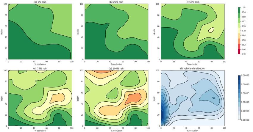
Figure 2. Generation pipeline for the ProcSy dataset: a) data priors that are used for procedural modeling; b) CityEngine is the program
used to generate three-dimensional, procedurally-generated world map; c) UE4 and CARLA are used for realistic lighting and weather
effects; d) dataset generation through CARLA is controlled via Python-based scripting; e) each frame of our dataset have the outlined
images rendered

   Berkeley Deep Drive [27] provides a finely-annotated                tains 13,400 random road scene annotated images that are
dataset comprised of 5683 images. This dataset has more                synthetically generated with various lighting and weather
weather and lighting variations than Cityscapes, but is noted          conditions. This dataset was updated in 2017 with the re-
to contain severe labeling inconsistencies in dark regions             lease of SYNTHIA-SF containing 2224 new images [15].
[24]. Similar to Mapillary, the BDD100K dataset does not               However, the dataset does not provide metadata quantify-
contain metadata with which the variations can be mea-                 ing lighting and weather variations, which are necessary to
sured. Thus, this dataset is also not conducive to measuring           study their influence on predictions.
the performance of a network against controlled weather                    Another approach has been to leverage an existing game
and lighting variations. In contrast, our dataset contains             environment. Examples include Playing for Data and sub-
metadata about both weather and lighting variations, using             sequently Playing for Benchmark datasets, developed using
a consistent annotation scheme (Sec. 4.2).                             the Grand Theft Auto V game environment by Richter et
                                                                       al. in 2016 and 2017 [21, 22]. In total, the latest state of
3.2. Synthetic Data Generation                                         their research contains 254,064 images. Angus et al. pro-
                                                                       posed a different and more salable method of data genera-
   In attempting to study effects of various influence fac-            tion from GTAV in 2018, and published a dataset with more
tors, including weather and lighting conditions, the realm             than 1,000,000 images in ideal weather and lighting condi-
of synthetic dataset generation appears promising. This is             tions [1]. A drawback of using existing games is that their
because variations in a synthetic environment are easier to            optimized and closed-source nature does not allow for eas-
control and quantify. One such example dataset is Virtual              ily controlling both the content and the rendering process.
KITTI [11] released in 2016. It is a virtual recreation of
the KITTI dataset [12] with the additional benefit that they           4. Generating the ProcSy Dataset
replicate each frame in 8 different weather and lighting vari-
ations. In total, Virtual KITTI currently has 21,260 frames               In this section, we detail the steps summarized in Fig. 2
[16] of semantically labeled data. In their paper, they pro-           for generating the ProcSy dataset.
vide an impact analysis of weather and imaging conditions
                                                                       4.1. Procedural Modeling for World Generation
on object tracking algorithms. However, they do not pro-
vide any analysis on semantic segmentation, as we have                    The generation of ProcSy begins with creating a virtual
done in our experiments. As another example from 2016,                 environment from which to capture road scene imagery.
Ros et al. published the SYNTHIA dataset [23], which con-              Our intent is to build a dataset with emphasis on scene varia-

                                                                     90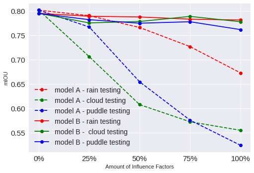
tion, therefore we do not focus on temporal frames. Instead,       in an energy-conservative manner to simulate physics of
we collect images by teleporting the camera around a stat-         light in the real world. Further, using an open-source sim-
ically built 3D environment. We choose to only focus on            ulation platform such as CARLA streamlines the process
building an environment with statically placed assets. This        of dataset generation. CARLA leverages UE4’s depth and
eliminates the effort needed to develop vehicle and pedes-         stencil buffers to output scene depth and automatic seman-
trian animation and traffic system controls.                       tic annotations. This provides us with the platform for our
    We used a procedural modeling tool called CityEngine           dataset generation (Fig. 2d-e).
(Fig. 2b). As explained in Sec. 2.2, procedural modeling
takes a set of grammar rules and iterates to create rich pat-      4.3. Vehicle Instances and Occlusion Maps
terns. In the case of CityEngine, these patterns represent a           We generate instance-level segmentation for the vehicle
three-dimensional derivation of city-scale maps.                   class. UE4 has the capability of rendering metallic mate-
    OpenStreetMap data [13] is fed into CityEngine as prior        rial buffer output. We leverage the idea of PBR materials
input (Fig. 2a). This data contains macroscopic information        and UE4’s metallic buffer output in order to label vehicle
about building footprints and road networks within a city re-      models as instance groups (i.e., all instances of a specific
gion. We chose a 3 km2 region of urban Canada (Fig. 3) as          vehicle model have the same label). By assigning each ve-
the template to model our virtual environment. Additional          hicle model’s material to a different specularity value, we
data priors were fed into CityEngine using Shapefiles [10]         can have a different metallic buffer id per vehicle model.
from municipal open databases. These data priors include           Additionally, we create a post-effect edge detection filter
such things as building heights and tree plantations.              using a combination of Sobel and Laplacian edge detection
    CityEngine stitches data priors together in order to create    algorithms. The resulting edges can be used to further break
a three-dimensional representation of the real-world coun-         up the instance groups into individual instances. A space-
terpart. For ProcSy, it took about one-person hour to iden-        saving measure, we encode ground truth data annotations,
tify and collect the relevant priors. The time-consuming as-       vehicle per-model instance ids, and edge detections in the
pect of procedural modeling is to restructure road networks        same PNG file (called the GT ID image in Fig. 2e), where
by accounting for lane-level details. Such reconstruction is       each takes up one of the RGB channels.
needed because OpenStreetMap does not contain lane-level               For our dataset, there are 43 unique vehicle models in
data, such as number of lanes, street/lane-width, or heights       use. We create a post-effects filter to generate occlusion
of overpasses and highways.                                        maps of vehicle models. We step through each of the unique
    Due to data unavailability, CityEngine cannot automati-        vehicle models and use this filter to output occlusions for
cally create exact road network layouts. A solution to this        each frame that contains the corresponding vehicle model.
may be to use high-definition (HD) maps with lane-level            As such, for each frame of the dataset, we have a set of
details. However, HD map data in an open-source format is          occlusion maps for vehicle models that appear in the frame.
still not readily available in the public domain. Currently,       We use these occlusion maps in one of the experiments in
the most cost-effective approach to this problem is using          Sec. 5.2.
openly available satellite imagery of road networks. Thus,
we used satellite imagery as a reference to manually adjust        4.4. Data Selection
the road graphs in CityEngine. This step took one person               Data points are selected such that the camera is always
approximately 40 hours for the 3 km2 geographical area.            facing towards a road-scene. The binary map in Fig. 3
                                                                   is derived from a top-down render of the 3 km2 map re-
4.2. Generating Ground Truth and Depth Data
                                                                   gion. In its original resolution of 4545×4541 pixels, there
   After the 3D environment has been generated and                 are 1,349,841 unique camera positions that can be chosen
populated with static vehicle and pedestrian models in             (white pixels). At each road-going (white) pixel, the top 2
CityEngine, these are exported to Unreal Engine 4 (UE4;            optimal orientations were determined by a simple line trac-
Fig. 2c). Doing so enables us to have more interaction             ing algorithm. A longer, unobstructed line trace (a black
with the rendering pipeline. CityEngine uses a traditional         pixel causes obstruction) is assumed to be a more optimal
rendering approach with a simplified lighting model to al-         orientation. Afterwards, one optimal orientation was cho-
low real-time rendering of massive amounts of geometry.            sen at random for each road-going pixel.
This means that end result of the render has limited realism.          From the set of 1,349,841 road scenes, using uniform
Also, CityEngine’s renderer currently does not support sim-        random sampling, crude renders were first taken to iden-
ulating rain and other adverse weather effects.                    tify 11,000 clean frames for our experimental dataset. This
   Unreal Engine 4 relies on Physically-Based Rendering            identification process required a human-in-the-loop to en-
(PBR) [19] to approximate a realistic lighting model. Tex-         sure frames did not have spawning issues with statically
tures and materials used throughout UE4 assets are rendered        placed assets such as vehicles and pedestrians. An exam-

                                                                  91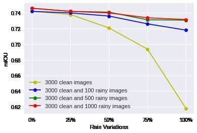
Figure 4. road scene frame approximately showing the Sun posi-
                                                                     tions in and out of frame that are considered; red x’s indicate Sun
                                                                     location and corresponding tuples show azimuth and altitude val-
                                                                     ues used in CARLA

                                                                         We also use the Sun’s position in the sky as another in-
                                                                     fluence factor (Fig. 4), consisting of the Sun’s azimuth and
                                                                     altitude angles. In order to reduce the amount of variations
                                                                     to study, we first make note of positions in a road scene
Figure 3. binary mask representing road-going pixels (white) of a    frame where the Sun’s angle and coincident shadow effects
3 km2 map region of urban Canada in top-down view; centered          are expected to have a meaningful impact. We note that be-
around (decimal degrees notation): 43.502507, -80.530754             low the horizon the Sun’s angle is irrelevant. Also, a typical
                                                                     road scene is expected to have buildings or other architec-
                                                                     ture along the left and right sides. These generally approach
ple non-clean frame would be the camera spawning inside              a vanishing point near center of the frame. Therefore, we
a statically placed road-going vehicle, which means all or           identify eight Sun positions within the frame that represent
most of the frame would show only the vehicle class.                 a V-shape in upper half of the frame. We also consider four
    Once clean frames were identified, the dataset was split         Sun positions outside the frame.
into a training set of 8000 frames, a validation set of 2000             With the identified environmental influence factor varia-
frames, and a test set of 1000 frames. In Fig. 3, frames from        tions, we can create 5×5×5×12=1500 unique RGB images
the bottom-right quadrant were used for validation and test          for each frame of our dataset. As explained in Sec. 5, we
sets. Frames from the other 3 quadrants were used for the            use a subset of this for our experimentation in order to en-
training set. The dataset was rendered in Cityscapes reso-           able faster experiment iterations.
lution (2048×1024 pixels) with the following outputs per
frame: RGB image (2.5mb), GT ID image (50kb), depth                  5. Analysis with ProcSy Dataset
map (790kb), and an occlusion maps folder (approx. 60kb)
containing n images where n refers to the number of unique              In this section, we present three experiments to demon-
vehicles that appear in the frame (Fig. 2e).                         strate the usage of our synthetic data for understanding dif-
                                                                     ferent effects of influence factors on semantic segmentation
4.5. Influence Factors Variations                                    model’s performance. For each of the three experiments we
   Our experimentation focuses on influence factor varia-            give the experimental objective, details, results, and actions
tions. We use CARLA’s capability to generate depth maps,             suggested by the results.
and we already discussed the generation of occlusion maps
                                                                     5.1. Effects of influence factors on model’s perfor-
for vehicle class in Sec. 4.3. The remaining influence fac-
                                                                           mance
tors are environmental ones, which we achieve with help
of existing UE4 functionality and CARLA. CARLA 0.9.1                    In this experiment, we train and compare the perfor-
introduced API calls to easily modify weather parameters             mance of two Deeplab v3+ models: model A is trained with
and Sun position in real-time (Fig. 2d). For ProcSy, we se-          8000 clean images, and model B is trained with 8000 im-
lected three weather influence factors, namely rain, cloud,          ages with equal proportion of three influence factors (rain,
and puddle deposits (accumulation of water on road pave-             cloud, and puddles). More precisely, model B’s training
ment). For each of these factors, we generate data for five          images are split into three equal parts, one per factor. Then
different intensity levels of 0%, 25%, 50%, 75%, and 100%.           each part is split in five equal sub-parts, one for a differ-

                                                                    92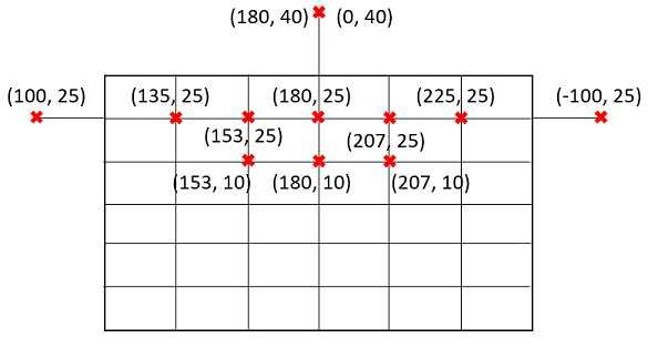
Figure 5. Performance of model A and B with different factors (each row); here, due to space constraints, we only show samples at 100%
level for each influence factor

ent level of the given factor to be applied: 0%, 25%, 50%,
75%, and 100%. Each model is trained with 140,000 itera-
tions with a batch-size of 16 and crop-size of 512×512. The
performance of each model is evaluated by testing with dif-
ferent influence factors. The purpose of this experiment is
two-fold. First, we would like to observe how the influence
factors degrade the performance of model A. Second, it is
important to know if model B is able to generalize across
different influence factors and is more robust than model A.
Otherwise, we would need to explore more advanced train-
ing methods to improve robustness, e.g., [28].
    In Fig. 6, we show mIoU of two models under differ-
ent testing conditions, where all test images have a certain
level of a influence factor. For model A, as we increase the
level of each influence factor, its performance worsens. Ini-         Figure 6. mIoU for each testing scenarios for two models, A and
tially, we found it surprising that cloud and puddle factors          B; x-axis denotes the intensity level of a given influence factor in
                                                                      each scenario
decrease the performance more than the rain factor does.
The reason for this is largely due to the model inaccurately
predicting sky as another class, such as car. This kind of            that model B was not trained with as many clean images as
error can be seen in Fig. 7, where we plot the IoU of sev-            model A. Overall, our results show that model B is more
eral classes for each model. For example, in Fig. 7, the              robust than model A.
IoU values of car and sky classes reduce significantly with
increased clouds compared to the other classes. Similarly,            5.2. Understanding the effect of occlusion and dis-
we can also see that puddles have a strong negative effect                  tance on network accuracy
on person, car, and road classes, because the puddle factor
creates reflection of objects on the ground. In contrast to               The ProcSy dataset allows for the assessment of the qual-
model A, model B has generally stable performance across              ity of a network’s prediction with respect to depth and oc-
all and different levels of factors, which suggests that the          clusion. Performing this analysis on an existing real-world,
model can generalize from the exposure to these factors in            autonomous driving dataset such as Cityscapes [6] is diffi-
training. Fig. 5 shows samples of each model’s predic-                cult since occlusion information is not available. However,
tion under different situations. We note that there is a small        this information can allow us to understand more about the
gap in overall and class-wise performance when testing on             reliability and weaknesses of a model.
clean images; however, this can be explained by the fact                  In this experiment, we randomly choose 270 im-

                                                                    93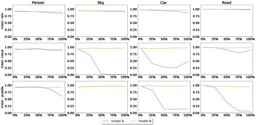
Figure 7. IoU values for 4 classes: person, sky, car and road; each row corresponds to each testing scenario (rain, cloud and puddle) and
each column corresponds to each class

Figure 8. ’a-e’ show model A’s accuracy on vehicles according to occlusion level and depth maps of the test set; darker green color
corresponds to higher accuracy; ’f’ shows frequency of vehicles in training set; scales for these plots are shown in color bars at the right.
The color bar for the distribution plot represents the distribution density.

ages with a total of 1200 vehicles in the test set. Also,                according to occlusion and depth (Fig. 8f). Similar to Syn-
we plot the distribution of vehicles in the training set                 scapes [26], we divide the predicted pixels into subsets of

                                                                       94
estimate this number.
We train and compare the performance of four different
models, one with 3000 clean images, and the other three
with the same 3000 clean images and an addition of 100,
500, or 1000 rainy images (each additional set containing
equal distribution of images at a given level: 25%, 50%,
75%, 100%) respectively. We further note that rainy im-
ages are created by randomly taking and modifying weather
conditions from the existing 3000 images, so that rain is the
only indicative feature that suggests any difference in the
performance between these models.
The results are shown in Fig. 9, where we can see
that most of the improvement could be obtained by adding
just 100 rainy images. For instance, when the amount of
Figure 9. mIoU values for each model of Sec.5.3 rain is 100%, it improves the performance by 10% (from
61.8% to 71.8% mIoU), whereas adding another 900 rainy
images only improves performance by an additional 2%.
[0%, 20%], [20%, 40%], [40%, 60%], [60%, 80%], [80%, 100%] Also, adding 1000 rainy images only gives us a slight
according to the depth and amount of occlusion of each increase in mIoU compared to adding only 500 images.
vehicle. Then, we calculate accuracy for each subset, after Since raindrops cause occlusion effects in the images (a
which we use cubic spline interpolation to get a contour kind of irreducible source of error), this result suggests that
plot. We repeat the same process for different levels of rain adding more rainy images will likely not further improve the
in the images, as shown in Fig. 8. model’s performance. By performing similar experiments
For the no rain case (Fig. 8a), generally we see that a for other influence factors, one can estimate the reasonable
higher amount of occlusion or depth will lower the model’s amount of real-world data that should be collected to im-
accuracy. Furthermore, the vehicle distribution shown in prove the robustness of a given model.
Fig. 8f indicates that depth and occlusion effects induce an
irreducible source of error. Specifically in Fig. 8f, although 6. Conclusions and Future Work
the right-most concentrated cluster has higher amount of
We presented an approach for rapidly producing a syn-
data than the bottom-most region, the model’s accuracy at
thetic replica of a real-world locale using procedural mod-
the right-most cluster in Fig. 8a is still lower than the accu-
eling in order to generate road scenes with different influ-
racy in the bottom region where there is little vehicle data.
ence factors and high-quality semantic annotations. We
Also, we observe that in the region bounded by used the approach to create ProcSy, a dataset for seman-
[0%, 20%] occlusion and [0%, 60%] depth, the model’s ac- tic segmentation with different influence factors, including
curacy is quite stable up until 50% rain amount (Fig. 8c). varying depth, occlusion, rain, cloud, and puddle levels.
This region corresponds to the left-most cluster in the dis- Our experiments show the utility of ProcSy to study the
tribution map (Fig. 8f). In general, the effects of rain re- effect of influence factors on the performance of Deeplab
duces the model’s performance significantly, especially for v3+, a state-of-the-art deep network for semantic segmen-
regions (in Fig. 8f) with little data. However, the degrada- tation. In our experiments, variations in puddle and cloud
tion effect of rain is counter-intuitive in some regions where levels affected the networks performance surprisingly more
the accuracies with high amounts of occlusion and depth are significantly than rain levels. Further, including as little
higher than regions with lower amounts of occlusion and as 3% of rainy images in the training set led to large im-
depth. For example, in Fig. 8e, the model’s accuracy in the provements of the networks robustness on such imagery (by
top-right region is higher than the middle-right region. This about 10%), whereas adding more than 15% of rainy images
is surprising and requires further investigation. showed signs of diminishing returns. This sort of knowl-
edge can be useful to determine how much real-world data
5.3. Estimating the amount of real-world data to be
for different influence factors to collect. This remains an
collected
exploration point for future work.
Collecting and labeling more data in different weather While this paper studied effects of influence factors in-
conditions is the simplest way to improve model’s robust- dividually, future work should explore their combinations.
ness. However, this is a costly and laborious task, and one Further exploration remains for understanding correlation
may want to know the optimal amount of data to collect. We of distribution densities of the factors on performance, as
show in this experiment how the ProcSy dataset can help us well as studying the effect of the factors in real-world data.
95References [17] G. Neuhold, T. Ollmann, S. Rota Bulò, and P. Kontschieder.
The mapillary vistas dataset for semantic understanding of
[1] M. Angus, M. ElBalkini, S. Khan, A. Harakeh, O. An- street scenes. In International Conference on Computer Vi-
drienko, C. Reading, S. L. Waslander, and K. Czarnecki. sion (ICCV), 2017. 2
Unlimited road-scene synthetic annotation (URSA) dataset.
[18] Y. I. H. Parish and P. Müller. Procedural modeling of cities.
CoRR, abs/1807.06056, 2018. 1, 3
In Proceedings of the 28th Annual Conference on Com-
[2] G. J. Brostow, J. Shotton, J. Fauqueur, and R. Cipolla. Seg- puter Graphics and Interactive Techniques, SIGGRAPH ’01,
mentation and recognition using structure from motion point pages 301–308, New York, NY, USA, 2001. ACM. 2
clouds. In ECCV (1), pages 44–57, 2008. 2 [19] M. Pharr, W. Jakob, and G. Humphreys. Physically based
[3] L. Chen, G. Papandreou, F. Schroff, and H. Adam. Re- rendering: From theory to implementation. Morgan Kauf-
thinking atrous convolution for semantic image segmenta- mann, 2016. 4
tion. CoRR, abs/1706.05587, 2017. 2 [20] P. Prusinkiewicz and J. Hanan. Lindenmayer systems, frac-
[4] L.-C. Chen, Y. Zhu, G. Papandreou, F. Schroff, and H. Adam. tals, and plants, volume 79. Springer Science & Business
Encoder-decoder with atrous separable convolution for se- Media, 2013. 2
mantic image segmentation. In Proceedings of the Euro- [21] S. R. Richter, Z. Hayder, and V. Koltun. Playing for bench-
pean Conference on Computer Vision (ECCV), pages 801– marks. In Proceedings of the IEEE International Conference
818, 2018. 2 on Computer Vision, pages 2213–2222, 2017. 1, 3
[5] F. Chollet. Xception: Deep learning with depthwise separa- [22] S. R. Richter, V. Vineet, S. Roth, and V. Koltun. Playing
ble convolutions. CoRR, abs/1610.02357, 2016. 2 for data: Ground truth from computer games. In B. Leibe,
[6] M. Cordts, M. Omran, S. Ramos, T. Rehfeld, M. Enzweiler, J. Matas, N. Sebe, and M. Welling, editors, European Con-
R. Benenson, U. Franke, S. Roth, and B. Schiele. The ference on Computer Vision (ECCV), volume 9906 of LNCS,
cityscapes dataset for semantic urban scene understanding. pages 102–118. Springer International Publishing, 2016. 3
In Proceedings of the IEEE conference on computer vision [23] G. Ros, L. Sellart, J. Materzynska, D. Vazquez, and
and pattern recognition, pages 3213–3223, 2016. 2, 6 A. Lopez. The SYNTHIA Dataset: A large collection of
[7] K. Czarnecki and R. Salay. Towards a framework to man- synthetic images for semantic segmentation of urban scenes.
age perceptual uncertainty for safe automated driving. In 2016. 3
SAFECOMP 2018 Workshops, WAISE, Proceedings, pages [24] C. Sakaridis, D. Dai, and L. V. Gool. Semantic night-
439–445, 2018. 1 time image segmentation with synthetic stylized data, grad-
[8] J. Deng, W. Dong, R. Socher, L.-J. Li, K. Li, and L. Fei-Fei. ual adaptation and uncertainty-aware evaluation. CoRR,
Imagenet: A large-scale hierarchical image database. 2009. abs/1901.05946, 2019. 1, 3
2 [25] F. Tung, J. Chen, L. Meng, and J. Little. The raincouver
[9] A. Dosovitskiy, G. Ros, F. Codevilla, A. Lopez, and scene parsing benchmark for self-driving in adverse weather
V. Koltun. CARLA: An open urban driving simulator. In and at night. IEEE Robotics and Automation Letters, PP:1–1,
Proceedings of the 1st Annual Conference on Robot Learn- 07 2017. 2
ing, pages 1–16, 2017. 1 [26] M. Wrenninge and J. Unger. Synscapes: A photorealistic
[10] E. ESRI. Shapefile technical description. An ESRI white synthetic dataset for street scene parsing. arXiv preprint
paper, 1998. 4 arXiv:1810.08705, 2018. 7
[11] A. Gaidon, Q. Wang, Y. Cabon, and E. Vig. Virtual [27] F. Yu, W. Xian, Y. Chen, F. Liu, M. Liao, V. Madhavan, and
worlds as proxy for multi-object tracking analysis. CoRR, T. Darrell. BDD100K: A diverse driving video database with
abs/1605.06457, 2016. 3 scalable annotation tooling. CoRR, abs/1805.04687, 2018. 3
[12] A. Geiger, P. Lenz, C. Stiller, and R. Urtasun. Vision meets [28] S. Zheng, Y. Song, T. Leung, and I. Goodfellow. Improving
robotics: The kitti dataset. The International Journal of the robustness of deep neural networks via stability training.
Robotics Research, 32(11):1231–1237, 2013. 3 In Proceedings of the ieee conference on computer vision and
[13] M. Haklay and P. Weber. Openstreetmap: User-generated pattern recognition, pages 4480–4488, 2016. 6
street maps. IEEE Pervasive Computing, 7(4):12–18, 2008.
4
[14] K. He, X. Zhang, S. Ren, and J. Sun. Deep residual learn-
ing for image recognition. In Proceedings of the IEEE con-
ference on computer vision and pattern recognition, pages
770–778, 2016. 2
[15] D. Hernandez-Juarez, L. Schneider, A. Espinosa,
D. Vazquez, A. Lopez, U. Franke, M. Pollefeys, and
J. C. Moure. Slanted stixels: Representing san franciscos
steepest streets. 2017. 3
[16] Naver. Proxy Virtual Worlds. http://www.europe.
naverlabs.com/Research/Computer-Vision/
Proxy-Virtual-Worlds. 3
96You can also read