Grad-TTS: A Diffusion Probabilistic Model for Text-to-Speech
←
→
Page content transcription
If your browser does not render page correctly, please read the page content below
Grad-TTS: A Diffusion Probabilistic Model for Text-to-Speech

              Vadim Popov * 1 Ivan Vovk * 1 2 Vladimir Gogoryan 1 2 Tasnima Sadekova 1 Mikhail Kudinov 1

                             Abstract                           2014) and Normalizing Flows (Rezende & Mohamed, 2015)
          Recently, denoising diffusion probabilistic mod-      were used in the design of TTS engines for a parallel gener-
          els and generative score matching have shown          ation with comparable quality of the synthesized speech.
          high potential in modelling complex data distri-      Since the publication of the WaveNet paper (2016), there
          butions while stochastic calculus has provided        have been various attempts to propose a parallel non-
          a unified point of view on these techniques al-       autoregressive vocoder, which could synthesize high-quality
          lowing for flexible inference schemes. In this        speech. Popular architectures based on Normalizing Flows
          paper we introduce Grad-TTS, a novel text-to-         like Parallel WaveNet (van den Oord et al., 2018) and Wave-
          speech model with score-based decoder produc-         Glow (Prenger et al., 2019) managed to accelerate inference
          ing mel-spectrograms by gradually transforming        while keeping synthesis quality at a very high level but
          noise predicted by encoder and aligned with text      demonstrated fast synthesis on GPU devices only. Eventu-
          input by means of Monotonic Alignment Search.         ally, parallel GAN-based vocoders such as Parallel Wave-
          The framework of stochastic differential equations    GAN (Yamamoto et al., 2020), MelGAN (Kumar et al.,
          helps us to generalize conventional diffusion prob-   2019), and HiFi-GAN (Kong et al., 2020) greatly improved
          abilistic models to the case of reconstructing data   the performance of waveform generation on CPU devices.
          from noise with different parameters and allows       Furthermore, the latter model is reported to produce speech
          to make this reconstruction flexible by explicitly    samples of state-of-the-art quality outperforming WaveNet.
          controlling trade-off between sound quality and
          inference speed. Subjective human evaluation          Among feature generators, Tacotron2 (Shen et al., 2018)
          shows that Grad-TTS is competitive with state-        and Transformer-TTS (Li et al., 2019) enabled highly nat-
          of-the-art text-to-speech approaches in terms of      ural speech synthesis. Producing acoustic features frame
          Mean Opinion Score.                                   by frame, they achieve almost perfect mel-spectrogram re-
                                                                construction from input text. Nonetheless, they often suffer
                                                                from computational inefficiency and pronunciation issues
1. Introduction                                                 coming from attention failures. Addressing these problems,
                                                                such models as FastSpeech (Ren et al., 2019) and Parallel
Deep generative modelling proved to be effective in various     Tacotron (Elias et al., 2020) substantially improved infer-
machine learning fields, and speech synthesis is no excep-      ence speed and pronunciation robustness by utilizing non-
tion. Modern text-to-speech (TTS) systems often consist of      autoregressive architectures and building hard monotonic
two parts designed as deep neural networks: the first part      alignments from estimated token lengths. However, in order
converts the input text into time-frequency domain acoustic     to learn character duration, they still require pre-computed
features (feature generator), and the second one synthe-        alignment from the teacher model. Finally, the recently
sizes raw waveform conditioned on these features (vocoder).     proposed Non-Attentive Tacotron framework (Shen et al.,
Introduction of the conventional state-of-the-art autoregres-   2020) managed to learn durations implicitly by employing
sive models such as Tacotron2 (Shen et al., 2018) used for      the Variational Autoencoder concept.
feature generation and WaveNet (van den Oord et al., 2016)
used as vocoder marked the beginning of the neural TTS          Glow-TTS feature generator (Kim et al., 2020) based on
era. Later, other popular generative modelling frameworks       Normalizing Flows can be considered as one of the most
such as Generative Adversarial Networks (Goodfellow et al.,     successful attempts to overcome pronunciation and com-
                                                                putational latency issues typical for autoregressive solu-
  *
   Equal contribution 1 Huawei Noah’s Ark Lab, Moscow, Rus-     tions. Glow-TTS model made use of Monotonic Alignment
      2
sia Higher School of Economics, Moscow, Russia. Correspon-      Search algorithm (an adoption of Viterbi training (Rabiner,
dence to: Vadim Popov , Ivan Vovk
.                                         1989) finding the most likely hidden alignment between
                                                                two sequences) proposed to map the input text to mel-
Proceedings of the 38 th International Conference on Machine    spectrograms efficiently. The alignment learned by Glow-
Learning, PMLR 139, 2021. Copyright 2021 by the author(s).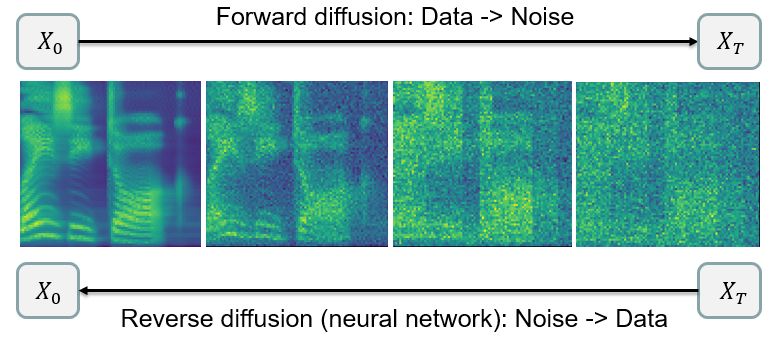
Grad-TTS: A Diffusion Probabilistic Model for Text-to-Speech
TTS is intentionally designed to avoid some of the pronun- Additionally, we show that it is possible to train Grad-TTS
ciation problems models like Tacotron2 suffer from. Also, as an end-to-end TTS pipeline (i.e., vocoder and feature
in order to enable parallel synthesis, Glow-TTS borrows generator are combined in a single model) by replacing its
encoder architecture from Transformer-TTS (Li et al., 2019) output domain from mel-spectrogram to raw waveform.
and decoder architecture from Glow (Kingma & Dhariwal,
2018). Thus, compared with Tacotron2, Glow-TTS achieves 2. Diffusion probabilistic modelling
much faster inference making fewer alignment mistakes.
Besides, in contrast to other parallel TTS solutions such as Loosely speaking, a process of the diffusion type is a
FastSpeech, Glow-TTS does not require an external aligner stochastic process that satisfies a stochastic differential equa-
to obtain token duration information as Monotonic Align- tion (SDE)
ment Search (MAS) operates in an unsupervised way.
Lately, another family of generative models called Diffusion dXt = b(Xt , t)dt + a(Xt , t)dWt , (1)
Probabilistic Models (DPMs) (Sohl-Dickstein et al., 2015)
has started to prove its capability to model complex data where Wt is the standard Brownian motion, t ∈ [0, T ] for
distributions such as images (Ho et al., 2020), shapes (Cai some finite time horizon T , and coefficients b and a (called
et al., 2020), graphs (Niu et al., 2020), handwriting (Luh- drift and diffusion correspondingly) satisfy certain measura-
man & Luhman, 2020). The basic idea behind DPMs is as bility conditions. A rigorous definition of the diffusion type
follows: we build a forward diffusion process by iteratively processes, as well as other notions from stochastic calculus
destroying original data until we get some simple distribu- we use in this section, can be found in (Liptser & Shiryaev,
tion (usually standard normal), and then we try to build a 1978).
reverse diffusion parameterized with a neural network so It is easy to find such a stochastic process that terminal dis-
that it follows the trajectories of the reverse-time forward tribution Law(XT ) converges to standard normal N (0, I)
diffusion. Stochastic calculus offers a continuous easy-to- when T → ∞ for any initial data distribution Law(X0 ) (I
use framework for training DPMs (Song et al., 2021) and, is n × n identity matrix and n is data dimensionality). In
which is perhaps more important, provides a number of fact, there are lots of such processes as it follows from the
flexible inference schemes based on numerical differential formulae given later in this section. Any process of the diffu-
equation solvers. sion type with such property is called forward diffusion and
As far as text-to-speech applications are concerned, two the goal of diffusion probabilistic modelling is to find a re-
vocoders representing the DPM family showed impressive verse diffusion such that its trajectories closely follow those
results in raw waveform reconstruction: WaveGrad (Chen of the forward diffusion but in reverse time order. This is,
et al., 2021) and DiffWave (Kong et al., 2021) were shown of course, a much harder task than making Gaussian noise
to reproduce the fine-grained structure of human speech and out of data, but in many cases it still can be accomplished
match strong autoregressive baselines such as WaveNet in if we parameterize reverse diffusion with a proper neural
terms of synthesis quality while at the same time requiring network. In this case, generation boils down to sampling
much fewer sequential operations. However, despite such a random noise from N (0, I) and then just solving the SDE
success in neural vocoding, no feature generator based on describing dynamics of the reverse diffusion with any nu-
diffusion probabilistic modelling is known so far. merical solver (usually a simple first-order Euler-Maruyama
scheme (Kloeden & Platen, 1992) is used). If forward and
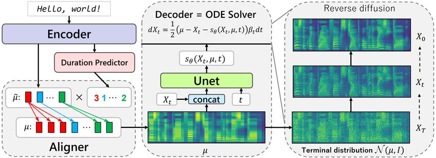
This paper introduces Grad-TTS, an acoustic feature gener- reverse diffusion processes have close trajectories, then the
ator with a score-based decoder using recent diffusion prob- distribution of resulting samples will be very close to that of
abilistic modelling insights. In Grad-TTS, MAS-aligned the data Law(X0 ). This approach to generative modelling
encoder outputs are passed to the decoder that transforms is summarized in Figure 1.
Gaussian noise parameterized by these outputs into a mel-
spectrogram. To cope with the task of reconstructing data Until recently, score-based and denoising diffusion proba-
from Gaussian noise with varying parameters, we write bilistic models were formalized in terms of Markov chains
down a generalized version of conventional forward and (Sohl-Dickstein et al., 2015; Song & Ermon, 2019; Ho et al.,
reverse diffusions. One of the remarkable features of our 2020; Song & Ermon, 2020). A unified approach introduced
model is that it provides explicit control of the trade-off be- by Song et al. (2021) has demonstrated that these Markov
tween output mel-spectrogram quality and inference speed. chains actually approximated trajectories of stochastic pro-
In particular, we find that Grad-TTS is capable of generating cesses satisfying certain SDEs. In our work, we follow
mel-spectrograms of high quality with only as few as ten this paper and define our DPM in terms of SDEs rather
iterations of reverse diffusion, which makes it possible to than Markov chains. As one can see later in Section 3, the
outperform Tacotron2 in terms of speed on GPU devices. task we are solving suggests generalizing DPMs described
in (Song et al., 2021) in such a way that for infinite timeGrad-TTS: A Diffusion Probabilistic Model for Text-to-Speech
By properties of Itô’s integral conditional distribution of Xt
given X0 is Gaussian:
Law(Xt |X0 ) = N (ρ(X0 , Σ, µ, t), λ(Σ, t)). (6)
It means that if we consider infinite time horizon
Rt then for
any noise schedule βt such that limt→∞ e− 0 βs ds = 0 we
have
d
Xt |X0 −
→ N (µ, Σ). (7)
Figure 1. Diffusion probabilistic modelling for mel-spectrograms.
So, random variable Xt converges in distribution to N (µ, Σ)
horizon forward diffusion transforms any data distribution independently of X0 , and it is exactly the property we need:
into N (µ, Σ) instead of N (0, I) for any given mean µ and forward diffusion satisfying SDE (2) transforms any data
diagonal covariance matrix Σ. So, the rest of this section distribution Law(X0 ) into Gaussian noise N (µ, Σ).
contains the detailed description of the generalized forward
and reverse diffusions we utilize as well as the loss function 2.2. Reverse diffusion
we optimize to train the reverse diffusion.
While in earlier works on DPMs reverse diffusion was
trained to approximate the trajectories of forward diffusion,
2.1. Forward diffusion Song et al. (2021) proposed to use the result by Anderson
First, we need to define a forward diffusion process that (1982), who derived an explicit formula for reverse-time
transforms any data into Gaussian noise given infinite time dynamics of a wide class of stochastic processes of the dif-
horizon T . If n-dimensional stochastic process Xt satisfies fusion type. In our case, this result leads to the following
the following SDE: SDE for the reverse diffusion:
1 p 1 −1
dXt = Σ−1 (µ − Xt )βt dt + βt dWt , t ∈ [0, T ] (2) dXt = Σ (µ − Xt ) − ∇ log pt (Xt ) βt dt
2 2 (8)
p
+ βt d W
ft , t ∈ [0, T ],
for non-negative function βt , which we will refer to as noise
schedule, vector µ, and diagonal matrix Σ with positive
elements, then its solution (if it exists) is given by where Wft is the reverse-time Brownian motion and pt is the
probability density function of random variable Xt . This
SDE is to be solved backwards starting from terminal con-
1 −1 t
R 1 −1 t
R dition XT .
Xt = I − e− 2 Σ 0 βs ds µ + e− 2 Σ 0 βs ds X0
Moreover, Song et al. (2021) have shown that instead of
Z tp (3)
+
1 −1 t
R
βs e− 2 Σ s βu du dWs . SDE (8), we can consider an ordinary differential equation
0
Note that the exponential of a diagonal matrix is just an 1 −1
dXt = Σ (µ − Xt ) − ∇ log pt (Xt ) βt dt. (9)
element-wise exponential. Let 2
Forward Kolmogorov equations corresponding to (2) and (9)
− 21 Σ−1
Rt
βs ds
are identical, which means that the evolution of probability
ρ(X0 , Σ, µ, t) = I − e 0 µ
(4) density functions of stochastic processes given by (2) and
− 12 Σ−1 0t βs ds (9) is the same.
R
+e X0
Thus, if we have a neural network sθ (Xt , t) that estimates
and the gradient of the log-density of noisy data ∇ log pt (Xt ),
then we can model data distribution Law(X0 ) by sampling
−1 t
R XT from N (µ, Σ) and numerically solving either (8) or (9)
λ(Σ, t) = Σ I − e−Σ 0 βs ds . (5) backwards in time.Grad-TTS: A Diffusion Probabilistic Model for Text-to-Speech
2.3. Loss function [1, F ] ∩ N and [1, L] ∩ N, and we put µj = µ̃A(j) for any in-
teger j ∈ [1, F ]. Informally speaking, the duration predictor
Estimating gradients of log-density of noisy data Xt is often
tells us how many frames each element of text input lasts.
referred to as score matching, and in recent papers (Song &
Monotonicity and surjectiveness of A guarantee that the text
Ermon, 2019; 2020) L2 loss was used to approximate these
is pronounced in the correct order without skipping any text
gradients with a neural network. So, in our paper, we use
input. As in all TTS models with duration predictor, it is
the same type of loss.
possible to control synthesized speech tempo by multiplying
Due to the formula (6), we can sample noisy data Xt given predicted durations by some factor.
only initial data X0 without sampling intermediate val-
The output sequence µ = µ1:F is then passed to the de-
ues {Xs }sGrad-TTS: A Diffusion Probabilistic Model for Text-to-Speech
Figure 2. Grad-TTS inference scheme.
3.2. Training encoder parameters. We use Monotonic Alignment Search
at the first step of this approach. MAS utilizes the concept of
One of Grad-TTS training objectives is to minimize the
dynamic programming to find an optimal (from the point of
distance between aligned encoder output µ and target mel-
view of loss function Lenc ) monotonic surjective alignment.
spectrogram y because the inference scheme that has just
This algorithm is described in detail in (Kim et al., 2020).
been described suggests to start decoding from random noise
N (µ, I). Intuitively, it is clear that decoding is easier if we To estimate the optimal alignment A∗ at inference, Grad-
start from noise, which is already close to the target y in TTS employs the duration predictor network. As in (Kim
some sense. et al., 2020), we train the duration predictor DP with Mean
Square Error (MSE) criterion in logarithmic domain:
If aligned encoder output µ is considered to parameterize
an input noise the decoder starts from, it is natural to regard
encoder output µ̃ as a normal distribution N (µ̃, I), which
leads to a negative log-likelihood encoder loss: F
X
di = log I{A∗ (j)=i} , i = 1, .., L,
j=1 (15)
F
X
Lenc = − log ϕ(yj ; µ̃A(j) , I), (14) Ldp = M SE(DP (sg[µ̃]), d),
j=1
where ϕ(·; µ̃i , I) is a probability density function of where I is an indicator function, µ̃ = µ̃1:L , d = d1:L and
N (µ̃i , I). Although other types of losses are also possi- stop gradient operator sg[·] is applied to the inputs of the
ble, we have chosen Lenc (which actually reduces to Mean duration predictor to prevent Ldp from affecting encoder
Square Error criterion) because of this probabilistic inter- parameters.
pretation. In principle, it is even possible to train Grad- As for the loss related to the DPM, it is calculated using
TTS without any encoder loss at all and let the diffusion formulae from Section 2. As already mentioned, we put
loss described further do all the job of generating realistic Σ = I, so the distribution of noisy data (6) simplifies, and
mel-spectrograms, but in practice we observed that in the its covariance matrix becomes just an identity matrix I
absence of Lenc Grad-TTS failed to learn alignment. multiplied by a scalar
The encoder loss Lenc has to be optimized with respect to
both encoder parameters and alignment function A. Since Rt
it is hard to do a joint optimization, we apply an iterative λt = 1 − e− 0
βs ds
. (16)
approach proposed by Kim et al. (2020). Each iteration
of optimization consists of two steps: (i) searching for an
optimal alignment A∗ given fixed encoder parameters; (ii) The overall diffusion loss function Ldif f is the expectation
fixing this alignment A∗ and taking one step of stochastic of weighted losses associated with estimating gradients of
gradient descent to optimize loss function with respect to log-density of noisy data at different times t ∈ [0, T ]:Grad-TTS: A Diffusion Probabilistic Model for Text-to-Speech
4. Experiments
" " ##
2 LJSpeech dataset (Ito, 2017) containing approximately
ξt
Ldif f = EX0 ,t λt Eξt sθ (Xt , µ, t) + √ , 24 hours of English female voice recordings sampled at
λt 2
22.05kHz was used to train the Grad-TTS model. The test
(17)
set contained around 500 short audio recordings (duration
where X0 stands for target mel-spectrogram y sampled from less than 10 seconds each). The input text was phone-
training data, t is sampled from uniform distribution on mized before passing to the encoder; as for the output
[0, T ], ξt – from N (0, I) and the formula acoustic features, we used conventional 80-dimensional
mel-spectrograms. We tried training both on original and
p normalized mel-spectrograms and found that the former per-
Xt = ρ(X0 , I, µ, t) + λt ξt (18)
formed better. Grad-TTS was trained for 1.7m iterations
on a single GPU (NVIDIA RTX 2080 Ti with 11GB mem-
is used to get noisy data Xt according to the distribution (6). ory) with mini-batch size 16. We chose Adam optimizer
The above formulae √ (17) and (18) follow from (12) and (10) and set the learning rate to 0.0001. The code will soon be
by substitution t = λt ξt . We use losses (12) with weights available at https://github.com/huawei-noah/
λt according to the common heuristics
h that these weights
i speech-backbones.
2
should be proportional to 1/E k∇ log p0t (Xt |X0 )k2 .
To sum it up, the training procedure consists of the following
steps:
• Fix the encoder, duration predictor, and decoder pa-
rameters and run MAS algorithm to find the alignment
A∗ that minimizes Lenc .
• Fix the alignment A∗ and minimize Lenc +Ldp +Ldif f
with respect to encoder, duration predictor, and decoder
parameters.
• Repeat the first two steps till convergence.
Figure 3. Diffusion loss at training.
3.3. Model architecture
As for the encoder and duration predictor, we use exactly We would like to mention several important things about
the same architectures as in Glow-TTS, which in its turn Grad-TTS training:
borrows the structure of these modules from Transformer-
TTS (Li et al., 2019) and FastSpeech (Ren et al., 2019) • We chose T = 1, βt = β0 + (β1 − β0 )t, β0 = 0.05
correspondingly. The duration predictor consists of two and β1 = 20.
convolutional layers followed by a projection layer that
predicts the logarithm of duration. The encoder is composed • As in (Bińkowski et al., 2020; Donahue et al., 2021),
of a pre-net, 6 Transformer blocks with multi-head self- we use random mel-spectrogram segments of fixed
attention, and the final linear projection layer. The pre-net length (2 seconds in our case) as training targets
consists of 3 layers of convolutions followed by a fully- y to allow for memory-efficient training. However,
connected layer. MAS and the duration predictor still use whole mel-
spectrograms.
The decoder network sθ has the same U-Net architecture
(Ronneberger et al., 2015) used by Ho et al. (2020) to gener- • Although diffusion loss Ldif f seems to converge very
ate 32 × 32 images, except that we use twice fewer channels slowly after the beginning epochs, as shown on Fig-
and three feature map resolutions instead of four to reduce ure 3, such long training is essential to get a good
model size. In our experiments we use 80-dimensional model because the neural network sθ has to learn to
mel-spectrograms, so sθ operates on resolutions 80 × F , estimate gradients accurately for all t ∈ [0, 1]. Two
40 × F/2 and 20 × F/4. We zero-pad mel-spectrograms models with almost equal diffusion losses can produce
if the number of frames F is not a multiple of 4. Aligned mel-spectrograms of very different quality: inaccurate
encoder output µ is concatenated with U-Net input Xt as an predictions for a small subset S ⊂ [0, 1] may have a
additional channel. small impact on Ldif f but be crucial for the output mel-Grad-TTS: A Diffusion Probabilistic Model for Text-to-Speech
spectrogram quality if ODE solver involves calculating Tacotron2. Furthermore, Grad-TTS-1000 achieves almost
sθ in at least one point belonging to S. natural synthesis with MOS being less than that for ground
truth recordings by only 0.1. We would like to note that
Once trained, Grad-TTS enables the trade-off between qual- the relatively low results of FastSpeech could possibly be
ity and inference speed due to the ability to vary the number explained by the fact that we used its unofficial implementa-
of steps N the decoder takes to solve ODE (13) at inference. tion https://github.com/xcmyz/FastSpeech.
So, we evaluate four models which we denote by Grad- To verify the benefits of the proposed generalized DPM
TTS-N where N ∈ [4, 10, 100, 1000]. We use τ = 1.5 at framework we trained the model with the same architecture
synthesis for all four models. As baselines, we take an of- as Grad-TTS to reconstruct mel-spectrograms from N (0, I)
ficial implementation of Glow-TTS (Kim et al., 2020), the instead of N (µ, I). The preference test provided in Table 1
model which resembles ours to the most extent among the shows that Grad-TTS-10 is significantly better (p < 0.005
existing feature generators, FastSpeech (Ren et al., 2019), in sign test) than this model taking 10, 20 and even 50
and state-of-the-art Tacotron2 (Shen et al., 2018). Recently iterations of the reverse diffusion. It demonstrates that the
proposed HiFi-GAN (Kong et al., 2020) is known to pro- model trained to generate from N (0, I) needs more steps
vide excellent sound quality, so we use this vocoder with all of ODE solver to get high-quality mel-spectrograms than
models we compare. Grad-TTS we propose. We believe this is because the task
of reconstructing mel-spectrogram from pure noise N (0, I)
4.1. Subjective evaluation is more difficult than the one of reconstructing it from its
noisy copy N (µ, I). One possible objection could be that
To make subjective evaluation of TTS models, we used the
the model trained with N (0, I) as terminal distribution can
crowdsourcing platform Amazon Mechanical Turk. For
just add µ to this noise at the first step of sampling (it is
Mean Opinion Score (MOS) estimation we synthesized 40
possible because sθ has µ as its input) and then repeat the
sentences from the test set with each model. The assessors
same steps as our model to generate data from N (µ, I). In
were asked to estimate the quality of synthesized speech on
this case, it would generate mel-spectrograms of the same
a nine-point Likert scale, the lowest and the highest scores
quality as our model taking only one step more. However,
being 1 point (“Bad”) and 5 points (“Excellent”) with a
this argument is wrong, since reverse diffusion removes
step of 0.5 point. To ensure the reliability of the obtained
noise not arbitrarily, but according to the reverse trajectories
results, only Master assessors were assigned to complete the
of the forward diffusion. Since forward diffusion adds noise
listening test. Each audio was evaluated by 10 assessors. A
gradually, reverse diffusion has to remove noise gradually
small subset of speech samples used in the test is available
as well, and the first step of the reverse diffusion cannot be
at https://grad-tts.github.io/.
adding µ to Gaussian noise with zero mean because the last
step of the forward diffusion is not a jump from µ to zero.
Table 1. Ablation study of proposed generalized diffusion frame-
work. Grad-TTS reconstructing data from N (0, I) for N reverse
diffusion iterations is compared with the baseline Grad-TTS-10 –
the model reconstructing data from N (µ, I) for 10 iterations.
N Worse, % Identical, % Better, %
10 93.8 0.5 5.7
20 82.3 2.9 14.8
50 60.3 5.7 34.0
MOS results with 95% confidence intervals are presented
in Table 2. It demonstrates that although the quality of the
synthesized speech gets better when we use more iterations
of the reverse diffusion, the quality gain becomes marginal
Figure 4. Typical errors occurrence.
starting from a certain number of iterations. In particular,
there is almost no difference between Grad-TTS-1000 and
Grad-TTS-10 in terms of MOS, while the gap between Grad- We also made an attempt to estimate what kinds of mis-
TTS-10 and Grad-TTS-4 (4 was the smallest number of iter- takes are characteristic of certain models. We compared
ations leading to satisfactory quality) is much more signifi- Tacotron2, Glow-TTS, and Grad-TTS-10 as the fastest
cant. As for other feature generators, Grad-TTS-10 is com- version of our model with high synthesis quality. Each
petitive with all compared models, including state-of-the-art record was estimated by 5 assessors. Figure 4 demon-Grad-TTS: A Diffusion Probabilistic Model for Text-to-Speech
Table 2. Model comparison.
Model Enc params1 Dec params RTF Log-likelihood MOS
Grad-TTS-1000 3.663 4.44 ± 0.05
Grad-TTS-100 0.363 4.38 ± 0.06
7.2m 7.6m 0.174 ± 0.001
Grad-TTS-10 0.033 4.38 ± 0.06
Grad-TTS-4 0.012 3.96 ± 0.07
Glow-TTS 7.2m 21.4m 0.008 0.082 4.11 ± 0.07
FastSpeech 24.5m 0.004 − 3.68 ± 0.09
Tacotron2 28.2m 0.075 − 4.32 ± 0.07
Ground Truth − − − 4.53 ± 0.06
strates the results of the multiple-choice test whose par- formation for all models under comparison. Additional
ticipants had to choose which kinds of errors (if any) they information regarding absolute inference speed dependency
could hear: sonic artifacts like clicking sounds or back- on the input text length is given in Figure 5.
ground noise (“sonic” in the figure), mispronunciation of
Due to its flexibility at inference, Grad-TTS is capable of
words/phonemes (“mispron”), unnatural pauses (“pause”),
real-time synthesis on GPU: if the number of decoder steps
monotone speech (“monotonic”), robotic voice (“robotic”),
is less than 100, it reaches RTF < 0.37. Moreover, although
wrong word stressing (“stress”) or others. It is clear from the
it cannot compete with Glow-TTS and FastSpeech in terms
figure that Glow-TTS frequently stresses words in a wrong
of inference speed, it still can be approximately twice faster
way, and the sound it produces is perceived as “robotic” in
than Tacotron2 if we use 10 decoder iterations sufficient for
around a quarter of cases. These are the major factors that
getting high-fidelity mel-spectrograms. Besides, Grad-TTS
make Glow-TTS performance inferior to that of Grad-TTS
has around 15m parameters, thus being significantly smaller
and Tacotron2, which in their turn have more or less the
than other feature generators we compare.
same drawbacks in terms of synthesis quality.
4.2. Objective evaluation
Although DPMs can be shown to maximize weighted varia-
tional lower bound (Ho et al., 2020) on data log-likelihood,
they do not explicitly optimize exact data likelihood. In
spite of this, Song et al. (2021) show that it is still possible
to calculate it using the instantaneous change of variables
formula (Chen et al., 2018) if we look at DPMs from the
“continuous” point of view. However, it is necessary to use
Hutchinson’s trace estimator to make computations feasible,
so in Table 2 log-likelihood for Grad-TTS comes with a
95% confidence interval.
We randomly chose 50 sentences from the test set and cal- Figure 5. Inference speed comparison. Text length is given in
culated their average log-likelihood under two probabilistic characters.
models we consider – Glow-TTS and Grad-TTS. Interest-
ingly, Grad-TTS achieves better log-likelihood than Glow-
TTS even though the latter has a decoder with 3x larger 4.4. End-to-end TTS
capacity and was trained to maximize exact data likelihood.
Similar phenomena were observed by Song et al. (2021) in The results of our preliminary experiments show that it
the image generation task. is also possible to train an end-to-end TTS model as a
DPM. In brief, we moved from U-Net to WaveGrad (Chen
4.3. Efficiency estimation et al., 2021) in Grad-TTS decoder: the overall architec-
ture resembles WaveGrad conditioned on the aligned en-
We assess the efficiency of the proposed model in terms coder output µ instead of ground truth mel-spectrograms
of Real-Time Factor (RTF is how many seconds it takes y as in original WaveGrad. Although synthesized speech
to generate one second of audio) computed on GPU and
1
the number of parameters. Table 2 contains efficiency in- Encoder and duration predictor parameters are calculated to-
gether.Grad-TTS: A Diffusion Probabilistic Model for Text-to-Speech
quality is fair enough, it cannot compete with the re- sentations, 2020.
sults reported above, so we do not include our end-to-end
model in the listening test but provide demo samples at Cai, R., Yang, G., Averbuch-Elor, H., Hao, Z., Belongie, S.,
https://grad-tts.github.io/. Snavely, N., and Hariharan, B. Learning Gradient Fields
for Shape Generation. In Proceedings of the European
Conference on Computer Vision (ECCV), 2020.
5. Future work
Chen, N., Zhang, Y., Zen, H., Weiss, R. J., Norouzi, M., and
End-to-end speech synthesis results reported above show Chan, W. WaveGrad: Estimating Gradients for Waveform
that it is a promising future research direction for text-to- Generation. In International Conference on Learning
speech applications. However, there is also much room for Representations, 2021.
investigating general issues regarding DPMs.
Chen, R. T. Q., Rubanova, Y., Bettencourt, J., and Duve-
In the analysis in Section 2, we always assume that both
naud, D. K. Neural Ordinary Differential Equations. In
forward and reverse diffusion processes exist, i.e., SDEs (2)
Advances in Neural Information Processing Systems, vol-
and (8) have strong solutions. It applies some Lipschitz-type
ume 31, pp. 6571–6583. Curran Associates, Inc., 2018.
constraints (Liptser & Shiryaev, 1978) on noise schedule
βt and, what is more important, on the neural network sθ . Donahue, J., Dieleman, S., Binkowski, M., Elsen, E., and
Wasserstein GANs offer an encouraging example of incor- Simonyan, K. End-to-end Adversarial Text-to-Speech. In
porating Lipschitz constraints into neural networks training International Conference on Learning Representations,
(Gulrajani et al., 2017), suggesting that similar techniques 2021.
may improve DPMs.
Elias, I., Zen, H., Shen, J., Zhang, Y., Jia, Y., Weiss, R.,
Little attention has been paid so far to the choice of the noise and Wu, Y. Parallel Tacotron: Non-Autoregressive and
schedule βt – most researchers use a simple linear sched- Controllable TTS, 2020.
ule. Also, it is mostly unclear how to choose weights for
losses (12) at time t in the global loss function optimally. A Goodfellow, I., Pouget-Abadie, J., Mirza, M., Xu, B.,
thorough investigation of such practical questions is crucial Warde-Farley, D., Ozair, S., Courville, A., and Bengio, Y.
as it can facilitate applying DPMs to new machine learning Generative Adversarial Nets. In Advances in Neural In-
problems. formation Processing Systems 27, pp. 2672–2680. Curran
Associates, Inc., 2014.
6. Conclusion Gulrajani, I., Ahmed, F., Arjovsky, M., Dumoulin, V., and
We have presented Grad-TTS, the first acoustic feature gen- Courville, A. C. Improved Training of Wasserstein GANs.
erator utilizing the concept of diffusion probabilistic mod- In Advances in Neural Information Processing Systems,
elling. The main generative engine of Grad-TTS is the volume 30, pp. 5767–5777. Curran Associates, Inc., 2017.
diffusion-based decoder that transforms Gaussian noise pa- Ho, J., Jain, A., and Abbeel, P. Denoising Diffusion Prob-
rameterized with the encoder output into mel-spectrogram abilistic Models. In Advances in Neural Information
while alignment is performed with Monotonic Alignment Processing Systems 33: Annual Conference on Neural
Search. The model we propose allows to vary the number Information Processing Systems 2020, NeurIPS 2020, De-
of decoder steps at inference, thus providing a tool to con- cember 6-12, virtual, 2020.
trol the trade-off between inference speed and synthesized
speech quality. Despite its iterative decoding, Grad-TTS is Ito, K. The LJ Speech Dataset, 2017. URL https://
capable of real-time synthesis. Moreover, it can generate keithito.com/LJ-Speech-Dataset/.
mel-spectrograms twice faster than Tacotron2 while keeping
synthesis quality competitive with common TTS baselines. Kim, J., Kim, S., Kong, J., and Yoon, S. Glow-TTS: A
Generative Flow for Text-to-Speech via Monotonic Align-
ment Search. In Advances in Neural Information Process-
References ing Systems 33: Annual Conference on Neural Informa-
Anderson, B. D. Reverse-time diffusion equation models. tion Processing Systems 2020, NeurIPS 2020, December
Stochastic Processes and their Applications, 12(3):313 – 6-12, virtual, 2020.
326, 1982. ISSN 0304-4149.
Kingma, D. P. and Dhariwal, P. Glow: Generative flow with
invertible 1x1 convolutions. In Advances in Neural In-
Bińkowski, M., Donahue, J., Dieleman, S., Clark, A., et al. formation Processing Systems 31: Annual Conference on
High Fidelity Speech Synthesis with Adversarial Net- Neural Information Processing Systems 2018, pp. 10236–
works. In International Conference on Learning Repre- 10245, 2018.Grad-TTS: A Diffusion Probabilistic Model for Text-to-Speech
Kloeden, P. E. and Platen, E. Numerical Solution of Stochas- Ronneberger, O., Fischer, P., and Brox, T. U-Net: Convo-
tic Differential Equations, volume 23 of Stochastic Mod- lutional Networks for Biomedical Image Segmentation.
elling and Applied Probability. Springer-Verlag Berlin In Medical Image Computing and Computer-Assisted
Heidelberg, 1992. Intervention – MICCAI 2015, pp. 234–241. Springer In-
ternational Publishing, 2015.
Kong, J., Kim, J., and Bae, J. HiFi-GAN: Generative Adver-
sarial Networks for Efficient and High Fidelity Speech Shen, J., Pang, R., et al. Natural TTS Synthesis by
Synthesis. In Advances in Neural Information Processing Conditioning WaveNet on Mel Spectrogram Predictions.
Systems 33: Annual Conference on Neural Information In 2018 IEEE International Conference on Acoustics,
Processing Systems 2020, NeurIPS 2020, December 6-12, Speech and Signal Processing (ICASSP), pp. 4779–4783,
virtual, 2020. April 2018.
Kong, Z., Ping, W., Huang, J., Zhao, K., and Catanzaro, Shen, J., Jia, Y., Chrzanowski, M., Zhang, Y., Elias, I., Zen,
B. DiffWave: A Versatile Diffusion Model for Audio H., and Wu, Y. Non-Attentive Tacotron: Robust and Con-
Synthesis. In International Conference on Learning Rep- trollable Neural TTS Synthesis Including Unsupervised
resentations, 2021. Duration Modeling. ArXiv, abs/2010.04301, 2020.
Sohl-Dickstein, J., Weiss, E., Maheswaranathan, N., and
Kumar, K., Kumar, R., de Boissiere, T., Gestin, L., et al.
Ganguli, S. Deep Unsupervised Learning using Nonequi-
MelGAN: Generative Adversarial Networks for Condi-
librium Thermodynamics. In Proceedings of the 32nd
tional Waveform Synthesis. In Advances in Neural Infor-
International Conference on Machine Learning, Pro-
mation Processing Systems 32, pp. 14910–14921. Curran
ceedings of Machine Learning Research, pp. 2256–2265.
Associates, Inc., 2019.
PMLR, 2015.
Li, N., Liu, S., Liu, Y., Zhao, S., and Liu, M. Neural Speech Song, Y. and Ermon, S. Generative Modeling by Estimating
Synthesis with Transformer Network. Proceedings of Gradients of the Data Distribution. In Advances in Neural
the AAAI Conference on Artificial Intelligence, 33:6706– Information Processing Systems, volume 32, pp. 11918–
6713, 07 2019. 11930. Curran Associates, Inc., 2019.
Liptser, R. and Shiryaev, A. Statistics of Random Processes, Song, Y. and Ermon, S. Improved Techniques for Train-
volume 5 of Stochastic Modelling and Applied Probabil- ing Score-Based Generative Models. In Advances in
ity. Springer-Verlag, 1978. Neural Information Processing Systems 33: Annual Con-
ference on Neural Information Processing Systems 2020,
Luhman, T. and Luhman, E. Diffusion models for Hand-
NeurIPS 2020, December 6-12, virtual, 2020.
writing Generation, 2020.
Song, Y., Sohl-Dickstein, J., Kingma, D. P., Kumar, A., Er-
Niu, C., Song, Y., Song, J., Zhao, S., Grover, A., and Ermon, mon, S., and Poole, B. Score-Based Generative Modeling
S. Permutation Invariant Graph Generation via Score- through Stochastic Differential Equations. In Interna-
Based Generative Modeling. In AISTATS, 2020. tional Conference on Learning Representations, 2021.
Prenger, R., Valle, R., and Catanzaro, B. Waveglow: A van den Oord, A., Dieleman, S., Zen, H., Simonyan, K.,
Flow-based Generative Network for Speech Synthesis. Vinyals, O., Graves, A., Kalchbrenner, N., Senior, A.,
In 2019 IEEE International Conference on Acoustics, and Kavukcuoglu, K. WaveNet: A Generative Model for
Speech and Signal Processing (ICASSP), pp. 3617–3621. Raw Audio. In 9th ISCA Speech Synthesis Workshop, pp.
IEEE, May 2019. 125–125, 2016.
Rabiner, L. A Tutorial on Hidden Markov Models and van den Oord, A., Li, Y., et al. Parallel WaveNet: Fast
Selected Applications. Proceedings of the IEEE, 1989. High-Fidelity Speech Synthesis. In Proceedings of the
35th International Conference on Machine Learning, vol-
Ren, Y., Ruan, Y., Tan, X., Qin, T., et al. FastSpeech: Fast, ume 80 of Proceedings of Machine Learning Research,
Robust and Controllable Text to Speech. In Advances pp. 3918–3926. PMLR, 10–15 Jul 2018.
in Neural Information Processing Systems 32, pp. 3171–
3180. Curran Associates, Inc., 2019. Yamamoto, R., Song, E., and Kim, J.-M. Parallel Wavegan:
A Fast Waveform Generation Model Based on Genera-
Rezende, D. J. and Mohamed, S. Variational inference with tive Adversarial Networks with Multi-Resolution Spec-
normalizing flows. In Proceedings of the 32nd Inter- trogram. In IEEE International Conference on Acoustics,
national Conference on Machine Learning, ICML 2015, Speech and Signal Processing (ICASSP), pp. 6199–6203,
Lille, France, 6-11 July 2015, pp. 1530–1538, 2015. 2020.You can also read