Semantic Localization Via the Matrix Permanent
←
→
Page content transcription
If your browser does not render page correctly, please read the page content below
Semantic Localization Via the Matrix Permanent
                       Nikolay Atanasov, Menglong Zhu, Kostas Daniilidis, and George J. Pappas
                                     GRASP Laboratory, University of Pennsylvania
                                           Philadelphia, PA 19104, USA
                             {atanasov,menglong,kostas,pappasg}@seas.upenn.edu

   Abstract—Most approaches to robot localization rely on low-        senses the environment. This and other traditional localization
level geometric features such as points, lines, and planes. In this   methods use vectors to represent the map and the sensor
paper, we use object recognition to obtain semantic information       measurements. Bayesian filtering in the resulting vector space
from the robot’s sensors and consider the task of localizing the
robot within a prior map of landmarks, which are annotated with       relies on the assumption that the data association, i.e., the
semantic labels. As object recognition algorithms miss detections     correspondence between the sensor observations and the fea-
and produce false alarms, correct data association between the        tures on the map, is known. While this might not be an issue
detections and the landmarks on the map is central to the             for scan matching in occupancy-grid maps, the assumption is
semantic localization problem. Instead of the traditional vector-     violated for landmark-based maps. Existing landmark-based
based representations, we use random finite sets to represent the
object detections. This allows us to explicitly incorporate missed    localization (and SLAM) techniques require external solutions
detections, false alarms, and data association in the sensor model.   to the problems of data association and clutter rejection [3, 25].
Our second contribution is to reduce the problem of computing             There is a line of work addressing visual localization,
the likelihood of a set-valued observation to the problem of          which matches observed image features to a database, whose
computing a matrix permanent. It is this crucial transformation       images correspond to the nodes of a topological map, e.g.
that enables us to solve the semantic localization problem with
a polynomial-time approximation to the set-based Bayes filter.        [40, 35, 2, 39, 24, 17]. Wang et al. [39] represent each location
The performance of our approach is demonstrated in simulation         in a topological map by a set of interest points that can be
and in a real environment using a deformable-part-model-based         reliably detected in images. A nearest neighbor search is used
object detector. Comparisons are made with the traditional lidar-     to match observed SIFT features to the database. Košecká
based geometric Monte-Carlo localization.                             and Li [17] also characterize scale-invariant key points by the
                                                                      SIFT descriptor and find nodes in the topological map, whose
                       I. I NTRODUCTION
                                                                      features match the observed ones the best. The drawback
   Localization, the problem of estimating the pose of a mobile       of maximum likelihood data association is that when it is
robot from sensor data given a prior map, is fundamental in           wrong it quickly causes the localization filter to diverge. Hesch
the field of robotics. Reliable navigation, object manipulation,      et al. [13] study the effects of unobservable directions on
mapping, and many other tasks require accurate knowledge of           the estimator consistency in vision-aided inertial navigation
the robot’s pose. Most existing approaches to localization and        systems. As object recognition algorithms miss detections and
the related simultaneous localization and mapping (SLAM)              produce false alarms, correct data association is crucial for
rely on low-level geometric features such as points, lines, and       semantic localization and semantic world modeling too [41].
planes and on precise metric maps, which store the geometric              Instead of the traditional vector-based representations, we
information. In contrast, we propose to use the recent advances       use random finite sets (RFS) to represent the semantic infor-
in object recognition to obtain semantic information from the         mation obtained from performing object recognition on the
robot’s sensors and localize the robot within a prior map of          robot’s observations. This allows us to explicitly incorporate
landmarks, which are annotated with semantic labels. This has         missed detections, false alarms, and data association in the sen-
several benefits. Localizing against semantically meaningful          sor model. In recent years, RFS-based solutions to SLAM have
landmarks is less ambiguous and helps with global localization        gained popularity due to their unified treatment of filtering and
and loop-closure. Also, high-precision sensors such as laser          data association. Mahler [23] derived the Bayesian recursion
range finders and 3-D lidars are not crucial for accurate             with RFS-valued observations and proposed a first-moment ap-
localization and can be replaced by regular cameras. Finally,         proximation, called the probability hypothesis density (PHD)
there is an abundance of maps for GPS-denied environments             filter. The PHD filter has been successfully applied to SLAM
which are semantically annotated, perhaps even sketched by            by Kalyan et al. [15], Lee et al. [20], and Mullane et al. [27].
hand, and could be used for the task. Maps can also be con-           In these works, the vehicle trajectory is tracked by a particle
structed via the semantic mapping approaches which received           filter and the first moment of a trajectory-conditioned map
significant attention in recent years [18, 12, 32, 29, 7].            for each particle is propagated via a Gaussian-mixture PHD
   Monte-Carlo localization based on geometric features was           filter. Bishop and Jensfelt [6] address geometric localization
introduced by Dellaert et al. [10]. The knowledge about the           by formulating hypotheses about the robot’s state and tracking
robot’s pose is represented by a weighted set of samples              them with the PHD filter. Zhang et al. [43] propose an
(particles) and is updated over time as the robot moves and           approach for visual odometry using a PHD filter to track SIFT
features extracted from observed images. None of these RFS-            The robot has access to a semantic map of the environment
based approaches have been applied in a semantic setting and           containing n objects with known poses and classes. Let the set
all rely on a first-moment approximation via the PHD filter.           Y = {y1 , . . . , yn } represent the map, where yi := (yip , yir , yic )
In addition to modeling semantic information, we carry out             consists of the position yip , orientation yir , and class yic of the
filtering with the full RFS observation model. Very few works          i-th object. Depending on the application, the object state yi
deal with the full model [9, 22, 36] and none have applied it to       may capture other observable properties of interest.
semantic localization or studied its computational complexity.            At each time t, the robot receives data from its sensors
    There are several related semantic localization approaches         and runs an object recognition algorithm, capable of detecting
which do not rely on an RFS model and do not explicitly                instances from the set of object classes C present in Y . If
handle data association problems. Anati et al. [1] match               some object y ∈ Y is visible and detected from the current
histogram of gradient energies and quantized colors features           robot pose xt , then the algorithm returns a detection zt . In
to expected features from the prior semantic map. Yi et al.            the remainder, we assume that a detection, zt := (ct , st , bt ),
[42, 16] use semantic descriptions of distance and bearing             consists of a detected class ct ∈ C, a detection score st ∈ S,
in a contextual map for active semantic localization. Bao              and an estimate bt ∈ B of the bearing from the sensor to
and Savarese [4] propose a maximum likelihood estimation               the detected object, where S is the range of possible scores
formulation for Semantic Structure from Motion. In addition            and B is the range of bearings, usually specified by the
to recovering the camera parameters (motion) and the 3-D               sensor’s field of view (e.g. a camera with B = [−47◦ , 47◦ ]
location of image features (structure), the authors recover the        was used in our experiments). Depending on the sensors and
3-D locations, orientations, and categories of objects in the          the visual processing, zt could also contain a bounding box,
scene. A Markov Chain Monte Carlo algorithm is used to                 range, color, or other information about the detected object.
solve a batch estimation problem by sampling from the data             Detections might also be generated by clutter, which includes
likelihood of the observed measurements.                               the background and any objects not captured on the map Y .
Summary of contributions:                                              Due to false alarms and misses, a randomly-sized collection
   • We represent the semantic information obtained from
                                                                       of detections is returned by the object recognition algorithm
      object recognition with random finite sets. This allows          at time t and is best represented by a random finite set Zt . For
      us to incorporate missed detections and data association         any t, denote the pdf of robot state xt conditioned on the map
      with the landmarks on the map in the sensor model.               Y , the past detections Z0:t , and the control history u0:t−1 by
   • We prove that obtaining the likelihood of a RFS-valued
                                                                       pt|t and that of xt | Y, Z0:t , u0:t by pt+1|t .
      observation is equivalent to a matrix permanent com-             Problem (Semantic Localization). Suppose that the control ut
      putation. It is this crucial transformation that enables         is applied to the robot at time t ≥ 0 and, after moving, the
      an efficient polynomial-time approximation to Bayesian           robot obtains a random finite set Zt+1 of detections. Given a
      filtering with set-valued observations.                          prior pdf pt|t and the semantic map Y , compute the posterior
   Connections between the matrix permanent and data asso-             pdf pt+1|t+1 which takes Zt+1 and ut into account.
ciation have been identified in the target tracking community
                                                                         It is natural to approach the semantic localization problem
[30, 8, 31, 26], [21, Ch.11] but this is the first connection with
                                                                       using recursive Bayesian estimation. This, however, requires
the random-finite-set observation model.
                                                                       a probabilistic model of the semantic observations, which
Paper Organization: In Sec. II we formulate the semantic               quantifies the likelihood of the random set Zt+1 of detections
localization problem precisely. In Sec. III we provide a proba-        conditioned on the set of objects Y and the robot state xt+1 .
bilistic model, which quantifies the likelihood of a random
finite set of object detections and captures false positives,                       III. S EMANTIC O BSERVATION M ODEL
missed detections, and unknown data association. The key               A. Observation Model for a Single Object Detection
relationship between filtering with the RFS observation model
                                                                          We begin by constructing a probabilistic model of the
and the matrix permanent is derived in Sec. IV. Finally, in
                                                                       semantic observations obtained from a single object in the
Sec. V, we present results from simulations and real-world
                                                                       environment. It consists of two ingredients: a detection model
experiments and discuss the performance of our approach.
                                                                       and an observation model. The detection model quantifies the
                      II. P ROBLEM F ORMULATION                        probability of detecting an object y ∈ Y from a given robot
   Consider a mobile robot, whose dynamics are governed                state x. Let β(x, y) be the true bearing from the robot’s sensor
by the motion model xt+1 = f (xt , ut , wt ), where xt :=              to the object y in the sensor frame1 . Let the field of view of
(xpt , xrt , xat ) is the robot state, containing its position xpt ,   the sensor2 be described by the set F oV (x). Objects outside
orientation xrt , and other variables xat such as velocity and           1 For example, in 2-D, assuming the robot and the sensor frames coincide,
acceleration, ut is the control input, and wt is the motion noise.     β(x, y) := | tan−1 ((xp(2) − y p(2) )/(xp(1) − y p(1) )) − xr |.
Alternatively, the model can be specified by the probability             2 The field of view of a camera in 2-D, assuming its frame coincides with the

density function (pdf) of xt+1 conditioned on xt and ut :              robot’s, can be represented by {w ∈ R2 | kxp − wk2 ≤ rd , β(x, w) ≤ αd },
                                                                       where αd is the angle of view and rd is the maximum range at which an
                          pf (· | xt , ut ).                    (1)    object can be detected.
the field of view cannot be detected. For the ones within, we              Let Yd (x) := {y ∈ Y | pd (y | x) > 0} be the set of detectable
 use a distance-decaying probability of detection:                          objects given a robot state x. We specify the pdf of Z for a
                 (          p  p     2
                                                                            series of increasingly more complex cases.
                   pd,0 e−ky −x k2 /σd if y p ∈ F oV (x),                      1) All measurements are clutter: If there are no objects in
    pd (y | x) =                                            (2)
                   0                    else,                               proximity to the sensor, i.e., Yd (x) = ∅, then any generated
                                                                            detections would be from clutter. The correct observation
 where pd,0 and σd2 are constants specifying the dependence of              model in this case is due to the Poisson clutter process:
 the detection probability on distance and are typically learned                                              Y
 from training data. The constants might depend on the object’s                            p(Z | ∅, x) = e−λ       λκ(z) .              (5)
 class y c but this is not explicit to simplify notation. A more                                                     z∈Z
 complex model which depends on the relative orientation                    This integrates to 1 if the set integral definition in [23,
 between x and y is also possible.                                          Ch.11.3.3] is used.
    Supposing that an object y ∈ Y is detected, the observation                2) No missed detections and no clutter: This is the case
 model quantifies the likelihood of the resulting detection                 of “perfect vision”, when every detectable object generates a
 z = (c, s, b) conditioned on the true object state y and the               detection, i.e. pd (y | x) ≡ 1 for any y ∈ F oV (x), and no
 robot state x. Assuming that conditioned on y, the bearing                 detections arise in any other way, i.e. λ = 0. If the number of
 measurement b is independent of the detected class c and the               detections m is not equal to the cardinality |Yd (x)| of the set
 detection score s, it is appropriate to model its conditional              of detectable objects, then p(Z | Yd (x), x) = 0 and otherwise:
 pdf pβ (· | y, x) as that of a Gaussian distribution with                                                    m
                                                                                                             XY
 mean β(x, y) and covariance Σβ . The covariance can be                               p(Z | Yd (x), x) =                pz (zπ(i) | yi , x),     (6)
 learned from training data and can be class dependent. Since                                                π i=1
 object recognition algorithms aim to be scale- and orientation-            where the sum is over all permutations π of the set {1, . . . , m}
 invariant, we can also assume that the detected class and score            and {y1 , . . . , ym } is an enumeration of Yd (x). For a derivation
 are independent of the robot state x. Then, the observation                see [23, Ch.12.3]. In general, it is not clear which of the de-
 model of the semantic measurement z can be decomposed as:                  tectable objects on the map produced which of the detections.
        pz (z | y, x) = pc (c | y c )ps (s | c, y c )pβ (b | y, x),   (3)   A permutation π specifies a particular correspondence between
                                                                            the m detectable objects and the m received detections. Intu-
 where pc (c | y c ) is the confusion matrix of the object detector         itively, all associations are plausible and we can think of (6) as
 and ps (s | c, y c ) is the detection score likelihood. The latter         quantifying the likelihood of Z by averaging the likelihoods
 can be learned for example by recording the detection scores               of the individual detections over all data associations.
 from the detected positive examples in a training set and using               3) No clutter but missed detections are possible: If m >
 kernel density estimation (see Fig. 7). Finally, a model of the            |Yd (x)|, then p(Z | Yd (x), x) = 0. If m = 0, then:
 pdf, κ(z), of a false positive detection generated by clutter is                                            |Yd (x)|
                                                                                                              Y
 needed. While it can also be learned from data, it is realistic                        p(∅ | Yd (x), x) =           (1 − pd (yi | x))           (7)
 to assume that clutter detections are uniformly distributed and                                              i=1
 independent of the robot’s state:
                                                                            and if m ∈ {1, . . . , |Yd (x)|}, then
                                 1 1 1
                         κ(z) =             .                         (4)     p(Z | Yd (x), x) =
                                |C| |S| |B|
                                                                                                     X    Y       pd (yi | x)pz (zπ(i) | yi , x)
 B. Observation Model for a Random Number of Detections                           p(∅ | Yd (x), x)                                               ,
                                                                                                     π i|π(i)>0
                                                                                                                       (1 − pd (yi | x))
   In this section we use Mahler’s finite set statistics [23] to
 model the pdf of a random finite set Z = {z1 , . . . , zm } of             where the sum is over all functions π : {1, . . . , |Yd (x)|} →
 object detections. The following assumptions are necessary:                {0, 1, . . . , m} with the property: π(i) = π(i0 ) > 0 ⇒ i = i0 ,
(A1) No detection is generated by more than one object                      which ensures that (A1) is satisfied. The index ‘0’ in the range
(A2) An object y ∈ Y generates either a single detection                    of π represents the case when a detectable object was missed.
      with probability pd (y | x) or a missed detection with                For example, it allows for the possibility that all detectable
      probability 1 − pd (y | x)                                            objects are missed (associated with ‘0’) and all m detections
(A3) The clutter process is Poisson-distributed in time with                are due to clutter.
                                                                               4) No missed detections but clutter is possible: If m <
      expected value λ and distributed in space according to
                                                                            |Yd (x)|, then p(Z | Yd (x), x) = 0; otherwise
      the pdf κ(z) in (4)
(A4) The clutter process and the object-detection process are                                                    X |YY
                                                                                                                     d (x)|
                                                                                                                            pz (zπ(i) | yi , x)
      statistically independent and all detections are condition-             p(Z | Yd (x), x) = p(Z | ∅, x)                                    ,
                                                                                                                                λκ(zπ(i) )
      ally independent given the object states                                                                   π   i=1
(A5) Any two detections in Z are independent conditioned on                 where the summation is over all one-to-one functions π :
      the map Y and the robot state x                                       {1, . . . , |Yd (x)|} → {1, . . . , m}.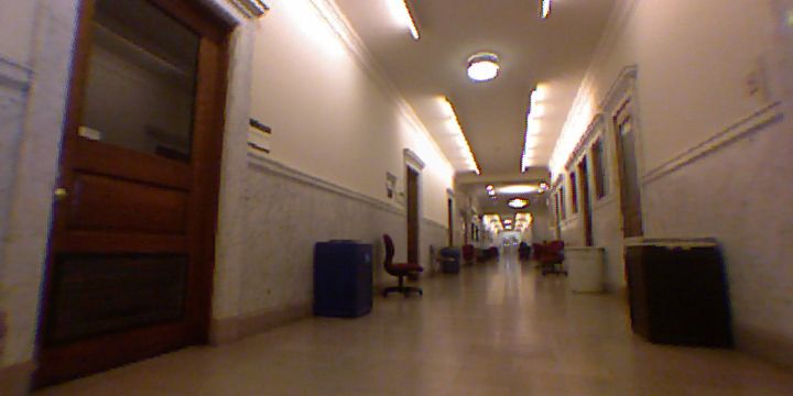
5) Both missed detections and clutter are possible: This         Algorithm 1 Set-based Particle Filter
is the most general model and captures all artifacts of object                                  k , xk }N , motion model pdf p , observation
                                                                     1: Input: Particle set {wt|t    t|t k=1                     f
recognition: missed detections, false positives, and unknown            model pdf p, semantic map Y , control input ut , detection set Zt+1
                                                                                                 k         k         N
                                                                     2: Output: Particle set {wt+1|t+1 , xt+1|t+1 }k=1
data association. If |Yd (x)| = 0, then the pdf is given by (5).
                                                                     3: for k = 1, . . . , N do
If m = 0, then the pdf is given by (7). Otherwise:                   4:     Predict: Draw xkt+1|t from pdf pf (· | xkt|t , ut )
                                                                     5:                 k
                                                                                     wt+1|t        k
                                                                                              ← wt|t
  p(Z | Yd (x), x) = p(Z | ∅, x)p(∅ | Yd (x), x)              (8)
                                                                            Update: wt+1|t+1 ← p Zt+1 | Yd (xkt+1|t ), xkt+1|t wt+1|t
                                                                                        k
                                                                                                                                 k
                                                                     6:
                     X Y pd (yi | x)pz (zπ(i) | yi , x)
                   ×                                         ,       7:              xkt+1|t+1 ← xkt+1|t
                                 (1 − pd (yi | x))λκ(zπ(i) )                                    k
                                                                     8: Normalize the weights {wt+1|t+1 }N
                      π   i|π(i)>0                                                                       k=1 and re-sample if necessary

where the sum is over all functions π : {1, . . . , |Yd (x)|} →
{0, 1, . . . , m} with the property: π(i) = π(i0 ) > 0 ⇒ i = i0 .   between the objects V1 and the measurements V2 or in other
    Having derived a general observation model for a random         words to perfect matchings3 in G. Given a perfect matching π,
number of object detections, we can now state the Bayesian          its associated product term inside the sum in (6) corresponds
filtering equations needed for semantic localization.               to its weight. Then, the sum over all π corresponds to the sum
                                                                    of the weights of all perfect matchings in G, which notably is
Proposition 1. The Bayesian recursion which solves the              equivalent to the permanent of the adjacency matrix of G.
Semantic Localization problem is:
                        Z                                           Definition 1 (Permanent). The permanent of an n × m matrix
Predict:    pt+1|t (x) = pf (x | x0 , ut )pt|t (x0 )dx0 (9)         A = [A(i, j)] with n ≤ m is defined as:
                                                                                                     n
Update: pt+1|t+1 (x) = ηt+1 p(Zt+1 | Yd (x), x)pt+1|t (x),                                          XY
                                                                                      per(A) :=              A(i, π(i)),
where p(Zt+1 | Yd (x), x) is the random finite set observation                                       π i=1
model in (8) and ηt+1 is a normalization constant.
                                                                    where the sum is over all one-to-one functions π : {1, . . . , n}
   IV. A PPROXIMATING THE S ET- BASED BAYES F ILTER                 → {1, . . . , m}. If n > m, then per(A) := per(AT ).
   While the Bayesian recursion with set-valued observations          It is now clear that the detection likelihood in the case of
in Prop. 1 is theoretically appealing, like its vector-based        no false positives and no missed detections can be obtained
counterpart it is intractable. An accurate and efficient approx-    by computing the permanent of a matrix.
imation to the set-based Bayes filter is therefore the subject of
this section. The particle filter [37, Ch.4] is an approximation    Proposition 2. The likelihood in (6) of a random finite set of
to the Bayes filter with vector-valued observations, which has      detections Z = {z1 , . . . , zm }, in the case of no false positives
been very successful for geometric localization. Since the          and no missed detections, with |Yd (x)| = m satisfies:
robot state is still vector-valued, we represent its pdf pt|t at
                                    k                                                   p(Z | Yd (x), x) = per(P ),
time t with a set of particles {wt|t  , xkt|t }N
                                               k=1 :

                             N                                      where P is a m × m matrix with P (i, j) := pz (zj | yi , x).
                             X
                                    k
                pt|t (x) ≈         wt|t δ(x   −   xkt|t ),             The general case in (8), where both false positives and
                             k=1
                                                                    missed detections are possible can be analyzed using the same
where δ(·) is a Dirac delta function. The particle filter im-       graph matching intuition. The following is our main result and
plementation of (9) with the motion model pf as a proposal          its proof appears in the Appendix.
distribution, is summarized in Alg. 1. It appears standard with
the exception that, instead of the conventional vector-based        Theorem 1. Given a robot state x and set of detectable objects
measurement update, line 6 requires computing the likelihood        Yd (x) with |Yd (x)| > 0, the likelihood of a random finite set
of the random set Zt+1 according to (8). In particular, it is       Z = {z1 , . . . , zm } of detections, with m > 0, when both
not apparent how to efficiently compute the sum over all            clutter and missed detections are possible satisfies:
associations π. To gain intuition we begin with the simpler
                                                                                              Y           Y
                                                                                           −λ
case of “perfect vision” in (6).                                     p(Z | Yd (x), x) = e           λκ(z)          (1 − pd (y | x))
                                                                                                 z∈Z            y∈Yd (x)
   Fix a robot state x and consider the non-trivial case when the
received measurements Z and the detectable landmarks Yd (x)                               1        Q              I|Yd (x)|
                                                                                        ×    per                                ,      (10)
are of the same cardinality m. Represent the sets Yd (x) and                              m!      1m,m          1m,|Yd (x)|
Z by the vertices of a complete (balanced) bipartite graph.
In detail, let V1 := Yd (x) and V2 := Z be the vertices             where λ is the expected number of clutter detections, κ(·) is
and E be the complete set of edges. Associate the weight            the spatial pdf of the clutter, pd (y | x) is the probability of
we := pz (z | y, x) with every edge e := (z, y) ∈ E and               3 A matching in graph G is a subgraph of G in which no two edges share
consider the weighted bipartite graph G := (V1 , V2 , E, w).        a common vertex. The weight of a matching is the product of all its edge
The permutations π in (6) correspond to different associations      weights. A matching is perfect if it contains all of G’s vertices.
detecting object y ∈ Yd (x), 1n,m is a n × m matrix of all Algorithm 2 Permanent (Nijenhuis and Wilf [28, Ch.23])
ones, and Q is a matrix with elements: 1: Input: n × n matrix A Output: per(A)
2: for i = 1, . . . , n do
pd (yi | x)pz (zj | yi , x) i = 1, . . . , |Yd (x)|, 3: x(i) ← A(i, n) − 12 n
P
j=1 A(i, j)
Q(i, j) := ,
(1 − pd (yi | x))λκ(zj ) j = 1, . . . , m, 4: s ← −1, g ← false(n, 1), p←s n
Q
i=1 x(i)
5: for k = 2, . . . , 2n−1 do
where without loss of generality it is assumed that |Yd (x)| ≤ 6: if k is even then j ← 1 . Obtain next gray code subset
m; otherwise re-label the sets Z and Yd . 7: else { j←2
8: while gj−1 is false do
Theorem 1 maps the problem of determining the pdf of Z in 9: j ←j+1 }
10: s ← −s, z ← 1 − 2gj , gj ← not gj
the general case in (8) to the problem of finding the permanent 11: for i = 1, . . . , n do
of a (m+|Yd (x)|)×(m+|Yd (x)|) square matrix. The problem 12: x(i) ← x(i) + zA(i, j)
is still computationally challenging because computing the p←p+s n
Q
13: i=1 x(i)
permanent of a matrix is #P-complete4 [38]. However, the 14: return 2(−1)n p
main advantage of Theorem 1 is that it allows us to lever-
age the extensive literature on approximation algorithms for encoders, a Kinect RGB-D camera with Nyko Zoom wide-
computing the matrix permanent. angle lens, and a Hokuyo UTM-30LX 2D laser range finder.
An exact method for computing the permanent of a n × n The IMU and the encoders were integrated using a differential
matrix, proposed by Ryser [34] and later improved by Nijen- drive model and Gaussian noise was added to obtain the mo-
huis and Wilf [28, Ch.23], is summarized in Alg. 2. Its time tion model in (1). In all experiments, the semantic localization
complexity is Θ(n2n−1 ). The dimension of the matrix in (10) was achieved using Alg. 1 with measurement updates obtained
is equal to the number of detections returned by the vision with the exact permanent algorithm (Alg. 2). Only the RGB
algorithm plus the number of detectable objects within the images were used for the semantic measurement updates. The
sensor field of view, which in practice is often small enough to depth was not used, while the lidar was used to provide
enable a real-time implementation of Alg. 2. Otherwise, there ground truth poses in the real-world experiments via geometric
are a number of polynomial-time arbitrarily-close approxima- Monte-Carlo localization. The performance of our approach
tions to the permanent computation. For example, Jerrum et al. is demonstrated for global localization, which means that the
[14] show that for any ∈ (0, 1] and δ > 0, there exists robot has absolutely no information about its starting pose.
a randomized algorithm whose output comes within a factor
B. Observation Model
(1 ± ) of per(A) with probability at least 1 − δ with a
random running time T such that E(T ) = O(n10 (log n)3 ). The state-of-the-art performance in single-image object
The running time was later improved by Bezáková et al. [5] detection is obtained by star-structured models such as de-
to O(n7 (log n)4 ). Also, when A ∈ [0, 1]n×n is a matrix such formable part models (DPM) [11]. Deformable part models
that all row and column sums are at least γn for γ ∈ (0.6, 1], were constructed for two object classes: C := {door, chair}
Law [19, Ch.2.2] provides an algorithm with expected running (Fig. 2). A DPM-based detector was used to process the RGB
time O(n4 (log n + −2 log δ −1 )). images obtained by the robot as follows. Given an input image,
an image pyramid is obtained via repeated smoothing and
Proposition 3. Given m object detections and a semantic map subsampling. Histograms of oriented gradients are computed
with n objects, the time complexity of Alg. 1 for semantic on a dense grid at each level of the pyramid. Detectors for the
localization with N particles is O(N (m + n)2(m+n) ) if the different classes in C are applied sequentially to the image,
measurement update is computed exactly with Alg. 2 and in a sliding-window fashion, and output detection scores at
O(N (n + m)7 (log(m + n))4 ) if computed approximately with each pixel and scale of the pyramid. Detection scores above
the method of Bezáková et al. [5]. a certain threshold are returned along with bounding box and
A final note on the computation of (10) is that the scaling bearing information. The collection of all such detections at
of the numbers can be improved by using that for a matrix time t forms the random finite set Zt . The detection model
A ∈ Rn×m and a constant γ, per(γA) = γ min(n,m) per(A). pd (y | x) and the observation model pz (z | y, x) were
In particular, some of the terms p(Z | ∅, x), p(∅ | Yd (x), x), obtained from training data as discussed in Sec. III-A. The
or 1/m! can be included within the permanent calculation. angle of view of the wide-angle lens was 94◦ , the detection
range - 10 meters, and the following constants were learned:
V. P ERFORMANCE E VALUATION pd,0 = 0.92, σd = 4.53, Σβ = 4◦ . The confusion matrix was:
A. Robot Platform
0.94 0.08
pc (c | y c ) =
We carried out simulations and real-world experiments in an 0.06 0.92
indoor environment using a differential drive robot equipped
while the detection score likelihood is shown in Fig. 7.
with an inertial measurement unit (IMU), magnetic wheel
C. Simulation Results
4A #P-complete problem is equivalent to computing the number of ac-
cepting paths of a polynomial-time nondeterministic Turing machine and #P The performance of the semantic localization algorithm was
contains NP. evaluated in a simulated environment of size 25 × 25 m2 ,0
meters
5
10
0 10 20 30 40 50 60
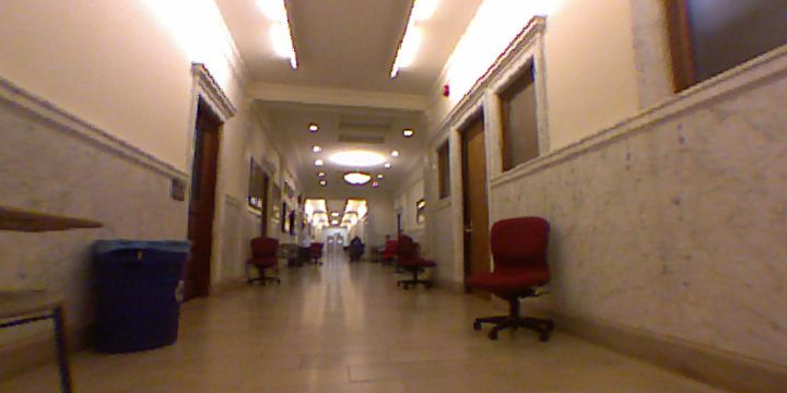
Fig. 1: Trajectories estimated by lidar-based geometric localization (red), image-based semantic Fig. 2: A component of the deformable
localization (blue), and odometry (green) from a real experiment. The starting position, the door part model of a chair
locations, and the chair locations are denoted by the red cross, the yellow squares, and the
blue circles, respectively. See the attached video or http://www.seas.upenn.edu/∼atanasov/vid/
RSS14 SemanticLocalization.mp4 for more details.
4 iterations 5 iterations 8 iterations 16 iterations
door door door door
door door door
door
door
door
chair chair chair
chair chair chair
Fig. 3: Particle filter evolution (bottom) and object detections (top) during a real semantic localization experiment
12 Iterations 17 Iterations 21 Iterations 26 Iterations 462 Iterations
20 20 20 20 20
10 10 10 10 10
0 0 0 0 0
−10 −10 −10 −10 −10
−20 −20 −20 −20 −20
−20 0 20 −20 0 20 −20 0 20 −20 0 20 −20 0 20
Fig. 4: A simulated environment with 45 objects from two classes (yellow squares, blue circles). The plots show the evolution of the particles
(red dots), the ground truth trajectory (green), and the estimated trajectory (red). The expected number of clutter detections was set to λ = 2.
6 Iterations 12 Iterations 18 Iterations 28 Iterations 462 Iterations
20 20 20 20 20
10 10 10 10 10
0 0 0 0 0
−10 −10 −10 −10 −10
−20 −20 −20 −20 −20
−20 0 20 −20 0 20 −20 0 20 −20 0 20 −20 0 20
Fig. 5: A simulated environment with 150 objects from 5 classes (circles, squares, triangles, crosses, and diamonds) in a 25 × 25 m2 area.
The plots show the particles (red dots), the ground truth trajectory (green), and the estimated trajectory (red) for clutter rate λ = 4.
2
RMSE [meters]
RMSE [meters]
4 Door True Class Chair
Position
Position
1
Door
2 0.1 0.1
0 0.05 0.05 0
0 100 200 300 400 0 20 40 60 80 100 120
Hypothesized Class
Time [sec]
20 0 0 15
−0.5 0 0.5 1 1.5 −0.5 0 0.5 1 1.5
RMSE [deg]
RMSE [deg]
Orientation
Orientation
10
10
5
0.1 0.1
0 0
0 100 200 300 400 0 20 40 60 80 100 120
0.05 0.05
Time [sec]
Chair
Iteration
Fig. 6: Root mean squared error (RMSE) in 0 0 Fig. 8: Root mean squared error (RMSE) be-
−0.5 0 0.5 1 1.5 −0.5 0 0.5 1 1.5
the pose estimates obtained from the semantic tween the pose estimates from semantic local-
Fig. 7: Detection score likelihoods learned
localization algorithm after 50 simulated runs ization and from lidar-based geometric local-
via kernel density estimation
of the scenario in Fig. 4 ization obtained from four real experiments3 Iterations 9 Iterations 16 Iterations 28 Iterations
20 20 20 20
0 0 0 0
−20 −20 −20 −20
−20 0 20 −20 0 20 −20 0 20 −20 0 20
Fig. 9: A simulated example of semantic localization in the presence of severe perceptual aliasing. The ground truth trajectory (blue) and
the evolution of the particle positions (red points) and orientations (red lines, top left) are shown.
TABLE I: Comparison of maximum likelihood data association
populated by objects with randomly-chosen positions and (MLD) and our random finite set approach (RFS) on the 4 real
classes (see Fig. 4). The error in the estimates averaged over datasets (Fig. 1) and the simulations in Fig. 4 and Fig. 9. Two
50 repetitions with different randomly-generated scenes is types of initializations were used: local (L), for which the initial
particle set had errors of up to 1 m and 30◦ , and global (G), for
presented in Fig. 6. Since the localization starts with a uniform
which the initial particle set was uniformly distributed over the whole
prior over the whole environment the error is large in the environment. Number of particles (NP) in thousands, position error
initial iterations. Multiple hypotheses are present until the (PE), orientation error (OE), and filter update time5 (UT), averaged
robot obtains enough detections to uniquely localize itself. The over time, are presented. The first MLD(G) column uses the same
performance in a challenging scenario with a lot of ambiguity number of particles as RFS(G), while the second uses a large number
in an attempt to improve the performance.
is presented in Fig. 9. The reason for using only two classes is
Fig. 1 MLD(L) MLD(G) MLD(G) RFS(L) RFS(G)
to increase the ambiguity in the data association. Our approach NP [K] 0.50 3.00 40.0 0.50 3.00
can certainly handle more classes and a higher object density. PE [m] 0.26 22.9 0.31 0.26 0.26
While the complexity in Prop. 3 is in terms of the total number OE [deg] 2.54 107 2.75 2.67 2.69
UT [sec] 0.023 0.060 0.600 0.065 0.320
of objects in the environment, the filter update times actually Fig. 4
scale with the density of the detectable objects. Fig. 5 shows NP [K] 0.50 5.00 100 0.50 5.00
PE [m] 15.3 24.9 17.3 0.32 0.72
a simulation with clutter rate λ = 4 and 150 objects from 5 OE [deg] 67.0 68.8 72.8 4.58 9.17
classes in a 25 × 25 m2 area. Scenarios with such high object UT [sec] 0.012 0.062 1.100 0.042 0.400
Fig. 9
density necessitate the use of an approximate, rather than the NP [K] 0.50 24.0 100 0.50 24.0
exact, permanent algorithm for real-time operation. PE [m] 0.27 48.8 26.9 0.11 2.35
OE [deg] 3.68 112 74.9 2.08 4.05
D. Experimental Results UT [sec] 0.027 0.760 3.340 0.062 2.620
In the real experiments, the robot was driven through a
long hallway containing doors and chairs. Four data sets were E. Comparison with Maximum Likelihood Data Association
collected from the IMU (at 100 Hz), the encoders (at 40 We compared our random finite set (RFS) approach to
Hz), the lidar (at 40 Hz), and the RGB camera (at 1 Hz). the more traditional maximum likelihood data association
Lidar-based geometric localization was performed via the amcl (MLD) approach used in FastSLAM [25]. MLD is based
package in ROS [33] and the results were used as the ground on Alg. 1 but the set of detections on line 6 is processed
truth. The lidar and semantic estimates of the robot trajectory sequentially. For each individual detection z, each particle x
are shown in Fig. 1. The error between the two, averaged over with weight w determines the most likely data association:
the 4 runs, is presented in Fig. 8. The error is large initially q := maxy∈Yd (x) pz (z | y, x) and updates its weight: w0 = qw.
because, unlike the lidar-based localization, our method was The performance is presented in Table I for two types of
started with an uninformative prior. Nevertheless, after the initializations: local (L), for which the initial particle set had
initial global localization stage, the robot is able achieve errors of up to 1 m and 30◦ , and global (G), for which it was
average errors in the position and orientation estimates of less uniformly distributed over the environment. MLD(L) performs
than 35 cm and 10◦ , respectively. The particle filter evolution as well as RFS(L) in the real experiments and in Fig. 9. In Fig.
is illustrated in Fig. 3 along with some object detections. 4, the data association is highly multimodal and MLD(L) does
In our experiments, it was sufficient to capture only class not converge even with 15K particles. This is reinforced in the
and position information in the object state because the ori- global initialization cases. While RFS(G) performs well with
entation and appearance variations were handled well by the 3K particles, MLD(G) needs 40K to converge consistently on
DPM. We emphasize that our model can incorporate richer the real datasets and is slower at the same level of robustness.
object representations by extending the state y and training In Fig. 4 and Fig. 9, MLD(G) does not converge even with
an appropriate observation model. This is likely to make the 100K particles. We conclude that once the particles have
data association more unimodal. As permanent approximation converged correctly MLD performs as well as RFS. However,
methods rely on Monte-Carlo sampling from the data asso- with global initialization or ambiguous data association MLD
ciations, fewer samples can be used in this case to speed up
the computations. Our reduction to the permanent incorporates 5 The reported times are from a MATLAB implementation on a PC with i7
this naturally and leverages state of the art algorithms. CPU@2.3GHz and 16GB RAMmakes mistakes and can never recover while RFS is robust where the assumption that |Yd (x)| ≤ m is used. The follow-
with a small number of particles. ing two lemmas describe a reduction from the problem of
summing all subpermanent sums of a rectangular matrix (or
VI. C ONCLUSION matchings in an unbalanced bipartite graph) to the problem of
Modeling the semantic information obtained from object the permanent of a rectangular matrix (or perfect matchings
detection with random finite sets enabled a unified treatment in an unbalanced bipartite graph) and then to the problem of
of filtering, data association, missed detections, and false the permanent of a square matrix (or perfect matchings in a
positives. The efficient implementation of the set-based Bayes balanced bipartite graph).
filter depends critically on the connection between the matrix
Lemma 1. Let An,m be an n × m matrix with n ≤ m. Then,
permanent and the RFS observation model. Simulations of
n
our approach showed precise and robust localization from X
perk (An,m ) = per( An,m In ).
semantic information in various scenarios and over many rep-
k=0
etitions. Compared to maximum likelihood data association,
our solution offers superior performance in cases of global Proof : Associate A with a weighted complete bipartite graph
localization, loop closure, and perceptual aliasing. The real GA := (V1 := {1, . . . , n}, V2 := {1, . . . , m}, E, wA ), where
experiments demonstrated that the accuracy of the semantic the weights wA corresponding with the entries of A. To
localization method is comparable with the laser-based geo- obtain the graph GB associated with B := An,m In add
metric approaches. Future work will focus on extensions to n dummy nodes V3 to V2 and n edges of weight 1. For
semantic SLAM and active semantic localization. k ∈ {0, . . . , n}, fix subsets α ∈ Qk,n and β ∈ Qk,m using the
notation from Def. 2. A perfect matching in GB associated
ACKNOWLEDGMENTS with α and β corresponds to:
We gratefully acknowledge support by TerraSwarm, one of • A k-matching between α ∈ V1 and β ∈ V2 of weight
six centers of STARnet, a Semiconductor Research Corpo- per(A[α, β])
ration program sponsored by MARCO and DARPA and the • A (n − k)-matching between V1 \ α and V3 of weight 1
following grants: NSF-OIA-1028009, ARL RCTA W911NF- Then, per(B) is the sum of all perfect matchings in GB :
10-2-0016, NSF-DGE-0966142, and NSF-IIS-1317788. We n
X X n
X
thank Chris Clingerman for his help with the MAGIC robot. per(B) = per(A[α, β]) = perk (A),
k=0 β∈Qk,m k=0
P ROOF OF T HEOREM 1 α∈Qk,n
Let V1 := Yd (x) and V2 := Z be the vertices of a where the last equality follows directly from Def. 2.
weighted complete bipartite graph G := (V1 , V2 , E, w), where Lemma 2. Let An,m be an n × m matrix with n ≤ m. Then,
the weight we associated with e := (i, j) ∈ E is Q(i, j). The
functions π in (8) specify different associations between the 1 An,m
per(An,m ) = per
objects V1 and the detections V2 . The introduction of missed (m − n)! 1m−n,m
detections (‘0’ in the range of π) means that some detectable where 1m−n,m is a (m − n) × m matrix of all ones.
objects need not to be assigned to a detection in Z. As
any object could be missed, the associations π correspond to Proof : Associate A with a weighted complete bipartite graph
matchings in the graph G. Given a matching π, the associated GA := (V1 := {1, . . . , n}, V2 := {1, . . . , m}, E, wA ), where
product term inside the sum in (8) corresponds to the weight the weights wA correspond with the entries of A. Toobtain
T
of π. Then, the sum over all π corresponds to the sum of the graph GB associated with B := ATn,m 1Tm−n,m add
the weights of all matchings in G. The sum of the weights (m−n) dummy nodes V3 to V1 and (m−n)m edges of weight
of all matchings with k edges can be computed via the k-th 1. Fix a subset β ∈ Qm−n,m using the notation from Def. 2.
subpermanent sum of the adjacency matrix Q of G. A perfect matching in GB associated with β corresponds to:
• A n-matching between V1 and V2 \ β of weight
Definition 2 (Subpermanent Sum). Let A be an n × m non- per(A[V1 , V2 \ β])
negative matrix with n ≤ m and let Qk,n be the set of all • A (m−n)-matching between V3 and β of weight (m−n)!
subsets of cardinality k of 1, . . . , n. For α ∈ Qk,n and β ∈ Then, per(B) is the sum of all perfect matchings in GB :
Qk,m let A[α, β] := [A(αi , βj )]ki,j=1 be the corresponding X
k-by-k submatrix of A. Define per0 (A) := 1 and per(B) = (m−n)! per(A[V1 , V2 \β]) = (m−n)! per(A),
X β∈Qm−n,m
perk (A) := per(A[α, β]), k = 1, . . . , n
where the last equality follows directly from Def. 2.
α∈Qk,n ,β∈Qk,m
The proof is completed by combining the two reductions
The sum in (8) is then equal to the sum over all k-matchings: above to write the sum in (11) as:
|Yd (x)|
X Y pd (yi | x)pz (zπ(i) | yi , x) |YX
d (x)|
X 1 Q I|Yd (x)|
= perk (Q), (11) perk (Q) = per .
(1 − pd (yi | x))λκ(zπ(i) ) m! 1m,m 1m,|Yd (x)|
π i|π(i)>0 k=0 k=0R EFERENCES tion and Mapping. The International Journal of Robotics
Research, 29(10):1251–1262, 2010.
[1] R. Anati, D. Scaramuzza, K. Derpanis, and K. Daniilidis. [16] D. W. Ko, C. Yi, and I. H. Suh. Semantic Mapping
Robot Localization Using Soft Object Detection. In IEEE and Navigation: A Bayesian Approach. In IEEE/RSJ Int.
Int. Conf. on Robotics and Automation (ICRA), pages Conf. on Intelligent Robots and Systems (IROS), pages
4992–4999, 2012. 2630–2636, 2013.
[2] A. Angeli, S. Doncieux, J. Meyer, and D. Filliat. Visual [17] J. Košecká and F. Li. Vision Based Topological Markov
topological SLAM and global localization. In IEEE Int. Localization. In IEEE Int. Conf. on Robotics and Au-
Conf. on Robotics and Automation (ICRA), 2009. tomation (ICRA), volume 2, pages 1481–1486, 2004.
[3] T. Bailey. Mobile Robot Localisation and Mapping [18] I. Kostavelis and A. Gasteratos. Learning Spatially Se-
in Extensive Outdoor Environments. PhD thesis, The mantic Representations for Cognitive Robot Navigation.
University of Sydney, 2002. Robotics and Autonomous Systems, 61(12):1460 – 1475,
[4] S. Bao and S. Savarese. Semantic Structure from Motion. 2013.
In Computer Vision and Pattern Recognition (CVPR), [19] W. Law. Approximately Counting Perfect and General
2011. Matchings in Bipartite and General Graphs. PhD thesis,
[5] I. Bezáková, D. Štefankovič, V. Vazirani, and E. Vigoda. Duke University, 2009.
Accelerating Simulated Annealing for the Permanent and [20] C. Lee, D. Clark, and J. Salvi. SLAM With Dynamic
Combinatorial Counting Problems. In ACM-SIAM Sym- Targets via Single-Cluster PHD Filtering. IEEE Journal
posium on Discrete Algorithms, pages 900–907, 2006. of Selected Topics in Signal Processing, 7(3):543–552,
[6] A. Bishop and P. Jensfelt. Global Robot Localization 2013.
with Random Finite Set Statistics. In Int. Conf. on [21] M. Liggins, D. Hall, and J. Llinas. Handbook of
Information Fusion, 2010. Multisensor Data Fusion. Taylor & Francis, 2008.
[7] J. Civera, D. Galvez-Lopez, L. Riazuelo, J. Tardos, and [22] W.-K. Ma, B.-N. Vo, S. Singh, and A. Baddeley. Tracking
J. Montiel. Towards Semantic SLAM Using a Monocular an Unknown Time-Varying Number of Speakers Using
Camera. In IEEE/RSJ Int. Conf. on Intelligent Robots and TDOA Measurements: A Random Finite Set Approach.
Systems (IROS), pages 1277–1284, 2011. IEEE Trans. on Signal Processing, 54(9):3291–3304,
[8] J. Collins and J. Uhlmann. Efficient Gating in Data As- 2006.
sociation with Multivariate Gaussian Distributed States. [23] R. Mahler. Statistical Multisource-Multitarget Informa-
IEEE Trans. on Aerospace and Electronic Systems, 28 tion Fusion. Artech House, 2007.
(3):909–916, 1992. [24] G. Mariottini and S. Roumeliotis. Active Vision-based
[9] P. Dames, D. Thakur, M. Schwager, and V. Kumar. Robot Localization and Navigation in a Visual Memory.
Playing Fetch with Your Robot: The Ability of Robots In IEEE Int. Conf. on Robotics and Automation (ICRA),
to Locate and Interact with Objects. IEEE Robotics and 2011.
Automation Magazine, 21(2):46–52, 2013. [25] M. Montemerlo and S. Thrun. Simultaneous Localization
[10] F. Dellaert, D. Fox, W. Burgard, and S. Thrun. Monte and Mapping with Unknown Data Association Using
Carlo Localization for Mobile Robots. In IEEE Int. Conf. FastSLAM. In IEEE Int. Conf. on Robotics and Au-
on Robotics and Automation (ICRA), volume 2, 1999. tomation (ICRA), volume 2, pages 1985–1991, 2003.
[11] P. Felzenszwalb, R. Girshick, D. McAllester, and D. Ra- [26] M. Morelande. Joint Data Association Using Importance
manan. Object Detection with Discriminatively Trained Sampling. In Int. Conf. on Information Fusion, pages
Part-Based Models. IEEE Trans. on Pattern Analysis and 292–299, 2009.
Machine Intelligence (PAMI), 32(9):1627–1645, 2010. [27] J. Mullane, B.-N. Vo, M. Adams, and B.-T. Vo. Random
[12] C. Galindo, A. Saffiotti, S. Coradeschi, P. Buschka, Finite Sets for Robot Mapping & SLAM. Springer Tracts
J. Fernandez-Madrigal, and J. Gonzalez. Multi- in Advanced Robotics. Springer, 2011.
hierarchical Semantic Maps for Mobile Robotics. In [28] A. Nijenhuis and H. Wilf. Combinatorial Algorithms.
IEEE/RSJ Int. Conf. on Intelligent Robots and Systems Academic Press, 1978.
(IROS), pages 2278–2283, 2005. [29] A. Nüchter and J. Hertzberg. Towards Semantic Maps
[13] J. Hesch, D. Kottas, S. Bowman, and S. Roumeliotis. for Mobile Robots. Robotics and Autonomous Systems,
Towards Consistent Vision-Aided Inertial Navigation. In 56(11):915–926, 2008.
Algorithmic Foundations of Robotics X, volume 86 of [30] S. Oh, S. Russell, and S. Sastry. Markov Chain Monte
Springer Tracts in Advanced Robotics. 2013. Carlo Data Association for Multi-Target Tracking. IEEE
[14] M. Jerrum, A. Sinclair, and E. Vigoda. A Polynomial- Trans. on Automatic Control, 54(3):481–497, 2009.
time Approximation Algorithm for the Permanent of a [31] H. Pasula, S. Russell, M. Ostland, and Y. Ritov. Tracking
Matrix with Nonnegative Entries. Journal of the ACM, Many Objects with Many Sensors. In Proc. Int. Joint
51(4):671–697, 2004. Conf. on Artificial Intelligence (IJCAI), volume 2, pages
[15] B. Kalyan, K. Lee, and W. Wijesoma. FISST-SLAM: 1160–1167, 1999.
Finite Set Statistical Approach to Simultaneous Localiza- [32] A. Pronobis. Semantic Mapping with Mobile Robots.PhD thesis, KTH Royal Institute of Technology, 2011.
[33] M. Quigley, B. Gerkey, K. Conley, J. Faust, T. Foote,
J. Leibs, E. Berger, R. Wheeler, and A. Ng. ROS: an
open-source Robot Operating System. In Proc. Open-
Source Software Workshop Int. Conf. on Robotics and
Automation (ICRA), 2009.
[34] H. Ryser. Combinatorial Mathematics. Carus Mathe-
matical Monographs # 14. Mathematical Association of
America, 1963.
[35] S. Se, D. Lowe, and J. Little. Vision-Based Global
Localization and Mapping for Mobile Robots. IEEE
Transactions on Robotics, 21(3):364–375, 2005.
[36] H. Sidenbladh and S.-L. Wirkander. Tracking Random
Sets of Vehicles in Terrain. In Computer Vision and
Pattern Recognition Workshop, volume 9, pages 98–98,
June 2003.
[37] S. Thrun, W. Burgard, and D. Fox. Probabilistic
Robotics. MIT Press Cambridge, 2005.
[38] L. Valiant. The Complexity of Computing the Permanent.
Theoretical Computer Science, 8(2):189–1201, 1979.
[39] J. Wang, H. Zha, and R. Cipolla. Coarse-to-Fine Vision-
Based Localization by Indexing Scale-Invariant Features.
IEEE Trans. on Systems, Man, and Cybernetics, 36(2):
413–422, 2006.
[40] J. Wolf, W. Burgard, and H. Burkhardt. Robust Vision-
based Localization by Combining an Image Retrieval
System with Monte Carlo localization. IEEE Transac-
tions on Robotics, 21(2):208–216, 2005.
[41] L. Wong, L. Kaelbling, and T. Lozano-Pérez. Data
Assocation for Semantic World Modeling from Partial
Views. In International Symposium on Robotics Research
(ISRR), 2013.
[42] C. Yi, I. H. Suh, G. H. Lim, and B.-U. Choi. Active-
Semantic Localization with a Single Consumer-Grade
Camera. In IEEE Int. Conf. on Systems, Man and
Cybernetics, pages 2161–2166, 2009.
[43] F. Zhang, H. Stahle, A. Gaschler, C. Buckl, and A. Knoll.
Single Camera Visual Odometry Based on Random Fi-
nite Set Statistics. In IEEE/RSJ Int. Conf. on Intelligent
Robots and Systems (IROS), pages 559–566, 2012.You can also read