Quantifying the Location Error of Precipitation Nowcasts
←
→
Page content transcription
If your browser does not render page correctly, please read the page content below
Hindawi
Advances in Meteorology
Volume 2020, Article ID 8841913, 12 pages
https://doi.org/10.1155/2020/8841913

Research Article
Quantifying the Location Error of Precipitation Nowcasts

          Arthur Costa Tomaz de Souza , Georgy Ayzel , and Maik Heistermann
          University of Potsdam, Institute of Environmental Science and Geography, Potsdam 14476, Germany

          Correspondence should be addressed to Arthur Costa Tomaz de Souza; costatomazde@uni-potsdam.de

          Received 11 September 2020; Accepted 21 October 2020; Published 3 December 2020

          Academic Editor: Francesco Viola

          Copyright © 2020 Arthur Costa Tomaz de Souza et al. This is an open access article distributed under the Creative Commons
          Attribution License, which permits unrestricted use, distribution, and reproduction in any medium, provided the original work is
          properly cited.

          In precipitation nowcasting, it is common to track the motion of precipitation in a sequence of weather radar images and to
          extrapolate this motion into the future. The total error of such a prediction consists of an error in the predicted location of a
          precipitation feature and an error in the change of precipitation intensity over lead time. So far, verification measures did not allow
          isolating the extent of location errors, making it difficult to specifically improve nowcast models with regard to location prediction.
          In this paper, we introduce a framework to directly quantify the location error. To that end, we detect and track scale-invariant
          precipitation features (corners) in radar images. We then consider these observed tracks as the true reference in order to evaluate
          the performance (or, inversely, the error) of any model that aims to predict the future location of a precipitation feature. Hence,
          the location error of a forecast at any lead time Δt ahead of the forecast time t corresponds to the Euclidean distance between the
          observed and the predicted feature locations at t + Δt. Based on this framework, we carried out a benchmarking case study using
          one year worth of weather radar composites of the German Weather Service. We evaluated the performance of four extrapolation
          models, two of which are based on the linear extrapolation of corner motion from t − 1 to t (LK-Lin1) and t − 4 to t (LK-Lin4) and
          the other two are based on the Dense Inverse Search (DIS) method: motion vectors obtained from DIS are used to predict feature
          locations by linear (DIS-Lin1) and Semi-Lagrangian extrapolation (DIS-Rot1). Of those four models, DIS-Lin1 and LK-Lin4
          turned out to be the most skillful with regard to the prediction of feature location, while we also found that the model skill
          dramatically depends on the sinuosity of the observed tracks. The dataset of 376,125 detected feature tracks in 2016 is openly
          available to foster the improvement of location prediction in extrapolation-based nowcasting models.

1. Introduction                                                               The present study focuses on nowcasts that are based on
                                                                          field tracking. The performance (or skill) of field tracking
Forecasting precipitation for the imminent future (i.e.,                  techniques is mostly verified by comparing the forecast
minutes to hours) is typically referred to as precipitation               precipitation field Ft+Δt for time t + Δt against the observed
nowcasting. A common nowcasting technique is to track the                 precipitation field Ot+Δt at time t + Δt, where t is the forecast
motion of precipitation from a sequence of weather radar                  time and Δt is the lead time. A large variety of verification
images and to extrapolate that motion into the future [1]. For            measures have been suggested in the literature (see, e.g.,
that purpose, we often assume that the intensity of pre-                  [4, 5]). Most of them, however, struggle with disentangling
cipitation features in the most recent image remains con-                 different sources of error: when we compare Ft+Δt to Ot+Δt,
stant over the lead time period—an assumption commonly                    how can we know the cause of the disagreement? Was it our
referred to as “Lagrangian persistence” [2]. In Lagrangian                prediction of the future location of a precipitation feature, or
field tracking, a velocity vector is obtained for each pixel of a          was it how precipitation intensity changed over time? Some
precipitation field, and that vector field is used to extrapolate           verification scores, such as the Fractions Skill Score [6],
the motion of the entire precipitation field—as opposed to                 apply a metric over spatial windows of increasing size in
cell tracking in which contiguous high-intensity objects are              order to examine how the forecast performance depends on
tracked (see [3] for a discussion of both methods).                       the spatial scale. Yet, we still lack the ability to explicitly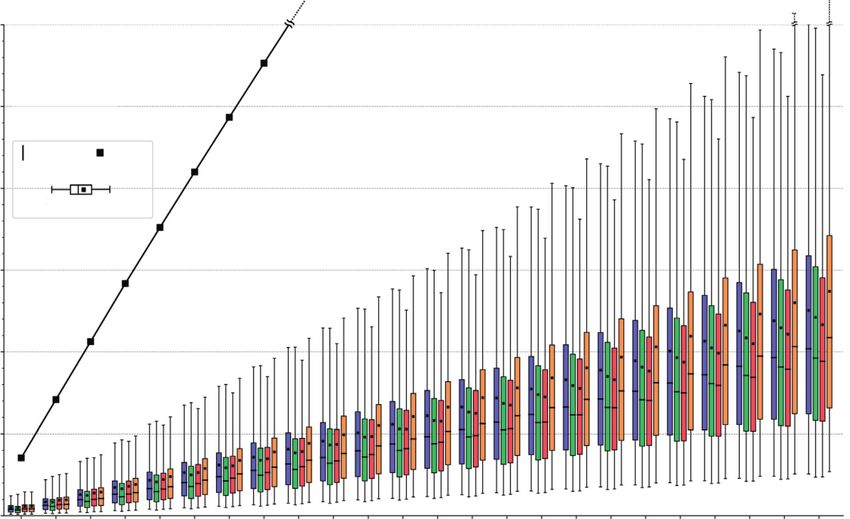
2                                                                                                                              Advances in Meteorology

isolate and quantify the location error. This makes it difficult                                                      True feature track
to benchmark and optimize the corresponding components
of nowcast models.                                                                                                                   Forecast feature track
    In this study, we introduce an approach to directly                                                               Location
                                                                                                                       error          t+3
quantify the location error of precipitation nowcasts which is
based on the extrapolation of field motion. With location                                                                       t+2
error, we refer to the spatial offset (or Euclidean distance)
between the true and the forecast locations of a precipitation                                                     t+1
                                                                            Forecast time                                  n
                                                                                                                        tio
feature (Figure 1). In this context, the term “feature” does
                                                                                             t                     p ola
                                                                                                                r a
not refer to a contiguous object but to a distinct point in the                                        e   xt
precipitation field, and we make use of the ability of the                           t–1         e   ar
                                                                          t–2               Lin
OpenCV library to detect and track the true motion of such
distinct points. In a verification case study, we will dem-           Figure 1: Illustration of the location error for a prediction at
onstrate the ability to quantify the location error by               forecast time t that is based on the linear extrapolation of feature
benchmarking a set of routine extrapolation techniques for           motion from t − 1 to t.
one year of quality-checked radar data in Germany.
    Section 2 highlights the approach to quantify the loca-              To collect all feature tracks T in any given time period
tion error and describes a set of tracking and extrapolation         with a length of n time steps, we detect “goodFeaturesTo-
techniques based on optical flow, as well as the radar data for       Track” (Shi and Tomasi, 1994) at each time step k ∈ [1, . . ., n],
our case study. Section 3 presents the results of our case           and track these features over as many subsequent time steps
study, and Section 4 concludes the paper.                            as possible. Accordingly, each track Ti,j,k could be identified
                                                                     by a unique tuple (i, j, k) that carries its starting point (by the
2. Methods and Data                                                  grid’s row and column indices, i and j) and its starting time
                                                                     index k. In this study, we use an analysis period of one year
2.1. Feature Detection and Tracking. We suggest quantifying          (2016, a leap year) and a time step length of 5 minutes, so
the location error of a forecast by comparing the observed           that k ∈ [1, . . ., 105408].
location (or displacement) of a precipitation feature against            In summary, the tracking process consists of six steps:
its predicted location. In visual computing, a feature is
defined as a point that stands out in a local neighborhood                (1) Identify the features pnew
                                                                                                    k   using goodFeaturesToTrack
and is invariant in terms of scale, rotation, and brightness                 [11] at any time k.
[7]. For a radar image, a feature (or corner) represents a               (2) If there are already features being tracked, pold
point with a sharp gradient of rainfall intensity [2].                                                                     k , from
                                                                             k − 1 to k, we consider only those features pnewk    for
     In this study, features are detected using the approach                 which the distance to any feature pold
of Shi and Tomasi [8] If a feature is detected at one time                                                         k is greater than
                                                                             7 km (with this threshold, we enforce consistency
step, we attempt to track that feature in any subsequent                     with the minDistance parameter of the Shi-Tomasi
time step until it is no longer trackable. The feature tracking
                                                                             corner detection; see Table 1). The trackable features
follows the approach of Kanade [9], as implemented by
                                                                             pk are hence the union of pold          new
                                                                                                            k and pk .
Bouguet [10]. The tracking error (or, inversely put, the
robustness of tracking a feature from one radar image to the             (3) Track pk from k to k + 1 using calcOpticalFlowPyrLK
next) is quantified in terms of the minimum eigenvalue of a                   [11];
2 × 2 normal matrix of optical flow equations (this matrix is             (4) Backwards track (from k + 1 to k) those features pk+1
called a spatial gradient matrix in Bouguet [10]), divided by                that were obtained in step 3.
the number of pixels in a neighborhood window. In the
tracking step, that minimum eigenvalue has to exceed a                   (5) Calculate the distance, dback , from the features pk to
threshold in order for a feature to be considered as suc-                    the backward-tracked locations resulting from step
cessfully tracked. Table 1 provides an overview of pa-                       4.
rameters used for both feature detection and tracking.                   (6) Keep only those features pk+1 where the distance
These values are based on the ones presented by Ayzel et al.                 dback is less than 1 km. These features are now pold
                                                                                                                              k+1 .
[2]. The underlying equations are well documented in
OpenCV [11].                                                              For statistical analysis, each track Ti,j,k is characterized by
     In order to increase the robustness of track detection, the     its duration τ (the number of time steps over which the track
tracking was also performed backwards at each time step              persists), the overall displacement distance d of the feature
(Figure 2): let pt signify a feature that was identified at frame t   along its track, the average feature velocity υ � d/τ, and the
and tracked to the next frame at time t + 1 at the position pt+1 .   straightness of the feature’s displacement in terms of the
The same tracking process was then applied backwards from            sinuosity index (SI) (which is calculated by dividing d by the
the point pt+1 to time t, yielding the point pback  t  . Only the    Euclidean distance between the feature origin and end lo-
trajectories where the distance dback between the source point       cations). The concept of sinuosity is widely used to char-
pt and the backwards tracked point pback   K    was less than one    acterize river curvatures as introduced by Mueller [12] and
kilometer (the grid resolution) were considered in our analysis.     was also applied to atmospheric science by Terry and Feng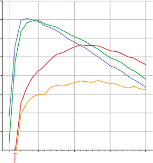
Advances in Meteorology                                                                                                                      3

                                 Table 1: OpenCV function parameters used for feature detection and tracking.
Parameter name                                    Value                                                    Meaning
maxCorners                                         200                                          Maximum number of features
qualityLevel                                       0.2                                      Minimum accepted quality of features
minDistance                                          7                                  Minimal Euclidean distance between features
blockSize                                           21                              Size of pixel neighborhood for covariance calculation
winSize                                          (20, 20)                                         Size of the search window
maxLevel                                            2                                        Maximal number of pyramid levels

                                                                                    Table 2: Overview of extrapolation models.
                    pt                               pt + 1
                                   Forward                                                                                    # Time steps
                                                                         Name                 Main approach
                                                                                                                              looking back
                                                                         Persist           Eulerian persistence                     0
            dback                         Backward                       LK-       Linear extrapolation based on Lukas
                                                                                                                                    1
                                                                         Lin1                     Kanade
                         pback
                          t                                              LK-       Linear extrapolation based on Lukas
                                                                                                                                    4
                                                                         Lin4                     Kanade
                                                                         DIS-         Linear extrapolation from DIS
                                                                                                                                    1
                                                                         Lin1                  motion field
                                                                                   Semi-Lagrangian extrapolation based
                                                                         DIS-
Figure 2: Illustration of the backward tracking test performed at                   on motion field obtained by dense                1
                                                                         Rot1
each time step for all features.                                                               optical flow

[13] to quantify the sinuosity of typhoon tracks. In our                 2.3.1. Eulerian Persistence. As a trivial benchmark, we use
analysis, we will also use the sinuosity index in order to               the assumption of Eulerian persistence, meaning that the
understand the error of predicted feature locations.                     precipitation feature will simply remain at its position at
                                                                         forecast time; that is, Pt+Δt � pt .

2.2. Error of Predicted Locations. Let p be the true location
and let P be the predicted location of a point feature in a              2.3.2. Linear Extrapolation. Linear extrapolation of feature
Cartesian coordinate system. At forecast time t, pt will be              motion assumes that a feature moves, over any lead time, at
equal to Pt. Consider Pt+Δt � f (pt, Δt, St) any function or             constant velocity and in the same direction. The displace-
algorithm that predicts the future location Pt+Δt of point pt            ment vector representing this motion can be obtained in
from any set St of predictors that is available at time t or             different ways. These ways constitute three different models
before. In the context of our study, that set of predictors              exemplified in the present study: LK-Lin1, LK-Lin4, and DIS-
could be, for example, the previous locations pt−1, pt−2, . . . of       Lin1. In the case of LK-Lin1 and LK-Lin4, the displacement
pt. We then define the error of our prediction, henceforth                vector is obtained from “looking back” m time steps from
referred to as location error ε, as the Euclidean distance               forecast time t to previous feature locations at t − m (tracked
between Pt+Δt and pt+Δt .                                                by using the Lucas–Kanade method, hence the LK label). For
                                                                         LK-Lin1, m equals 1, so the vector v(t, pt ) to displace feature
                                                                         pt is the connection from pt−1 to pt; for LK-Lin4, m equals 4,
2.3. Extrapolation Techniques. In a verification experiment,              so that the displacement vector results from the connection
we can use our collection of tracks T in order to retrieve               between pt−4 and pt, where the length of the vector is divided
points pt for which the location Pt+Δt at t + Δt should be               by 4 in order to obtain the displacement velocity. Hence, a
predicted, points that could be used as predictors (St), as well         forecast at lead time Δt extends the vector v(t, pt ) corre-
as the true location pt+Δt of the point at t + Δt. Assuming that         spondingly. Please see Figure 3 for an illustration of both the
an extrapolation of motion uses feature locations from m                 LK-Lin1 and the LK-Lin4 method. Of course, any other
time steps before t, the minimum feature track length to                 look-back time m could be used to obtain a displacement
produce a forecast would be m + 1. In order to retrieve the              vector. In this study, we arbitrarily used m ∈ {1, 4} in order to
location error of such a prediction at time t + Δt, we would             examine the effect of m on the forecast performance.
need a minimum track length of m + Δt + 1.                                    For the DIS-Lin1 model, a complete field of motion
    Based on the above terminology, we present in the                    vectors VDIS is obtained from the Dense Inverse Search
following the extrapolation models analyzed in the present               (DIS) method [14]; the underlying concept and equations of
study. These models are based on the models that were also               the DIS method have been elaborated by Kroeger et al. [15]
evaluated in a recent benchmarking study on optical-flow-                 and then used for the extrapolation. A point pt is linearly
based precipitation nowcasting [2]. Table 2 gives an overview            extrapolated from t to t + n by n times the velocity vector
of model acronyms and their main properties.                             vDIS (t, pt ), where vDIS (t, pt ) is the vector closest to pt in the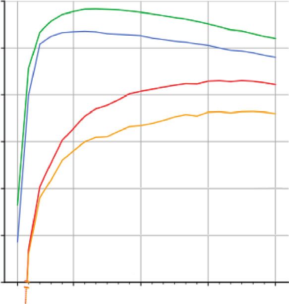
4                                                                                                                                       Advances in Meteorology

                                                    t+n                                                                     t + n ε (tn)
                                                                  ε (tn)
                                              t+3                                                                                      v (t)
                                                                                                                    v (t)          t
                                             t+2
               y                                                                                           v (t)            t–1
                                                                      v (t)   y
                                     t+1
                                                          v (t)                                v (t)
                                               v (t)                                                               t–2
                                 t
                                                                                       v (t)
                   t–1               v (t)                                                              t–3
                         v (t)
                                                                                      t–4
                                                   x                                                                 x
Figure 3: Illustration of the linear extrapolation schemes for the LK group: on the left LK-Lin1 and on the right LK-Lin4. The location error
is displayed by ε(tn).

VDIS (t) field (Figure 4). VDIS (t) is calculated by OpenCV’s
cv2.DISOpticalFlow_create function, which returns velocity                                                                     t+n
vectors for each grid pixel based on the radar frames from                                  VDIS (t)
t − 1 to t. In a recent benchmarking study about optical-flow-                                                            t+3
based precipitation nowcasting, Ayzel et al. [2] showed that                                                        t+2
the DIS-based model (referred to as the “Dense” model in
that paper) is an effective method for radar-based precipi-                        y
                                                                                                             t+1
tation nowcasting.
                                                                                                       t
                                                                                      t–1
2.3.3. Semi-Lagrangian Approach Based on Dense Optical
Flow. In a Semi-Lagrangian approach, the motion field is                                                                        x
typically assumed as constant over the forecast period and
the feature trajectory is determined by following the                         Figure 4: In the DIS-Lin1 model, the vector vDIS (t, pt ) (light red
streamlines [16]. Following this concept, the DIS-Rot1                        arrow) obtained from VDIS (t) is transferred to the pt location and
model (corresponding to “Dense rotation” in [2]) uses the                     linearly extended to t + n.
two most recent radar images, t − 1 and t, to estimate VDIS (t)
by cv2.DISOpticalFlow_create function. Similar to the DIS-                                                                     t+n
Lin1 model, the displacement vector vDIS (t, pt ) which is                               VDIS (t)
closest to pt is used to extrapolate the motion of pt from its                                                        t+3
position at t to t + 1, providing the location of Pt+1. This
                                                                                                                    t+2
process is repeated at all lead time steps until the maximum
lead time is achieved. Hence, at each lead time step n, we                        y                         t+1
retrieve the vector vDI S (t, Pt+n ) which is closest to Pt+n in
order to extrapolate the feature location, Pt+n+1 . Accord-                                         t
ingly, the velocity vector is updated at each lead time step                          t–1
from VDIS (t), allowing for rotational or curved motion
patterns (Figure 5).
                                                                                                                               x
                                                                              Figure 5: Schematic of the DIS-Rot1 model (orange path), where
2.4. Weather Radar Data and Experimental Setup. Our                           the velocity is updated every time step by transferring the velocity
benchmarking case study is based on weather radar data                        vector vDIS (t, p) (light orange arrow) closest to pt (black circles, for
from the German Weather Service, namely, the RY product                       t � 0) or Pt+1 (orange circles, for t > 0) in VDIS(t), to the Pt + Δt
generated as part of the RADKLIM radar reanalysis of the                      location to advect.
German Weather Service DWD [17]. The RY product
represents a quality-controlled national precipitation in-
tensity composite from 18 C-Band radars covering Germany                      mountains that would interfere with the beam propagation.
at 5-minute intervals and a spatial resolution of 1 km at an                  Quality control includes a wide range of correction methods
extent of 1100 × 900 km. The basis of the composite product                   for, e.g., clutter or partial beam blockage (see [17] for
is the so-called “precipitation scans” from each of the 18                    details).
radar locations. The precipitation scan is designed to follow                     The year 2016, selected for this experiment, was char-
the horizon as closely as possible at an azimuth resolution of                acterized by an annual precipitation close to the climato-
1° and a radial resolution of 1 km, adjusting the elevation                   logical mean for most regions in Germany, as can be seen in
angle for each azimuth depending on the presence of                           the German Climate Atlas [18]. However, the precipitation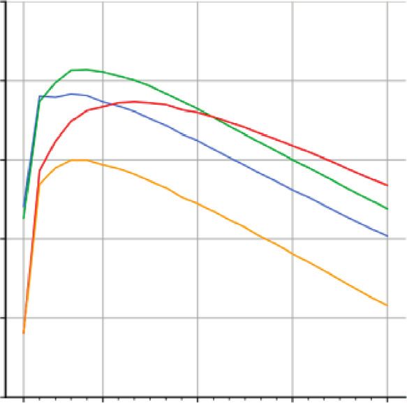
Advances in Meteorology                                                                                                           5

mean during autumn was below the normal average and                 general, expect the length of a track to increase with its
during the winter months slightly above the climatological          duration. Yet, there are also months—most notably the
mean.                                                               summer months from May to August—where this expec-
    As 2016 was a leap year, this experiment was carried out        tation is not met; and, of course, the length of a track de-
on 105408 radar composite images. Since none of the                 pends not only on its duration but also on a feature’s
methods under evaluation required any kind of training,             velocity. The average feature velocity in 2016 amounted to a
there was no need to split the data into sets for calibration       value of 42 km/h; and, in fact, not only does velocity show a
and validation. Instead, we used all tracks for verification.        clear seasonal pattern (with minimum velocities in the
For each track, we always use, as forecast time t, a time of 20     summer months; see Figure 6(d)), but also the seasonal
minutes after the feature was detected for the first time. That      pattern helps us to understand where the patterns of track
is because our model LK-Lin4 needs to look back four time           length and duration appear to be “inconsistent.” For ex-
steps (i.e., 20 minutes) in order to make a forecast, and we        ample, the track velocity is at a minimum in May and June,
need to make sure, for a fair comparison, to compare all            which decreases the length of track despite the rather high
models for the same forecast times.                                 duration values for these two months.
                                                                        The clearest seasonal pattern can be observed for rainfall
                                                                    intensity (Figure 6(e)). That pattern is very much in line with
2.5. Computational Details. The analysis was carried out in a       our expectation as rainfall in the summer months is gov-
Python 3.6 environment using the following main open-               erned by convective events that tend to be more intense than
source libraries: NumPy (https://numpy.org), NumExpr                stratiform event types. However, if we assumed that a higher
(https://github.com/pydata/numexpr), and SciPy (https://            rainfall intensity along a track is caused by the convective
www.scipy.org) for general computations; OpenCV                     nature of the underlying event, the track duration in the
(https://opencv.org) for feature tracking; and Pandas               corresponding months (e.g., May and June) is at least
(https://pandas.pydata.org) and h5py (https://www.h5py.             surprising: we would expect a convective event not only to be
org).                                                               more intense but also to be rather short (in comparison to
                                                                    widespread stratiform rainfall). The apparent inconsistency
3. Results and Discussion                                           between the patterns of rainfall intensity and track duration
                                                                    points us to one of the key issues with the presented track
3.1. Properties of Collected Tracks. The identification and          inventory: we must not misinterpret a “track” as an “event”
tracking process detected 376,125 features above the rainfall       in a hydrometeorological sense. The corner detection al-
rate threshold of 0.2 mm/h and lasted over 20 minutes,              gorithm (see Section 2.1) searches for pronounced features
which resulted in 337,776 eligible tracks after applying the        in the sense of strong local gradients and tracks a feature for
extrapolation step. A track was considered as “eligible” in         as long as it stands out. While we define a rainfall event as
case all models had a predicted location at all lead times,         some coherent process in space and time, the tracking al-
from t to t + n. The loss of 10.2% that is implied by the above     gorithm could “lose” a feature right in the course of an
numbers was caused by the DIS group of models which did             ongoing event and maybe, at the same time, find another
not generate a valid velocity vector vDIS (t, pt ) near every pt    feature to track somewhere else in the field. Obviously, the
point, in the VDIS (t) field, within a 3.5 km threshold.             tracking algorithm was able to track features over a longer
    Figure 6 gives an overview of the properties of the valid       duration in May, June, and September of 2016. However, as
tracks. The figure also shows the seasonal dependency of             of now, we do not know which properties of the corre-
these track properties by summarizing their distribution on         sponding rainfall events caused that effect. We should just
a per month basis. We would like to emphasize that this             emphasize that the duration of a track does not necessarily
analysis must not be interpreted as a “climatology” of track        correspond to the duration of an event. In the same way, we
properties as it only contains data from a single year. Still, we   cannot expect the tracking algorithm to find features at
consider it as illustrative to investigate which properties tend    “representative” locations of a convective cell. It will detect
to exhibit a seasonal pattern and also to discuss whether the       such features anywhere in a rainfall field where local gra-
observed properties can be considered as representative for         dients meet the tracking criteria. That could be right not only
the governing rainfall processes in Germany.                        in the middle of heavy rainfall but also at the edges. Hence,
    In an average month of 2016, we identified and tracked           the reported precipitation intensities along the tracks will
28,146 features (Figure 6(a)). The largest number of tracks is      not be representative of the mean precipitation intensities of
found from April to August (all above the average). Yet,            the corresponding precipitation fields.
there is no continuous seasonal pattern in the number of                Altogether, we have to emphasize at this point that the
detected tracks because, e.g., January and October also show        seasonal track statistics are indeed plausible. But it must be
rather large counts.                                                clear that track statistics are not necessarily representative
    No pattern at all can be found for the track length             for “event” statistics. That notion might be irritating for
(Figure 6(b)). With an average track length of 128 km,              those who have been defining and tracking features in terms
monthly maximum mean and median track lengths occur in              of coherent rainfall objects over their lifetime from initiation
January, April, and September. A partly similar pattern can         to dissipation. A new feature track as we understand it in our
be found for the track duration that amounts to 207 minutes         analysis could be found right in the middle of an ongoing
on average (Figure 6(c)). This is plausible as we would, in         event, and it can be lost long before the actual rainfall
6 Advances in Meteorology
Ave = 28146 Ave = 128
Jan 875.8
Jan Mean Median Feb 793.06
Feb 25% 95% Mar 774.18
Min Max
Mar 5% 75% Apr 869.54
Apr
May 882.9
May
Jun 825.71
Jun
Jul 969.44
Jul
Aug 963.59
Aug
Sep Sep 908.94
Oct Oct 1233.41
Nov Nov 812.08
Dec Dec 766.41
10000 20000 30000 40000 50000 0 100 200 300 400 500
Count Track length (km)
(a) (b)
Ave = 207 Ave = 42
Jan 1870 Jan 133.77
Feb 1685 Feb 135.21
Mar 1315 Mar 117.67
Apr 1350 Apr 115.16
May 1690 May 105.78
Jun 2235 Jun 108.56
Jul 1635 Jul 114.58
Aug 1040 Aug 111.83
Sep 1825 Sep 122.65
Oct 1955 Oct 130.8
Nov 2170 Nov 133.6
Dec 2605 Dec 137.57
0 200 400 600 800 0 25 50 75 100 125
Duration (min) Velocity (km/h)
(c) (d)
Ave = 1.6 Ave = 1.09
Jan 14.85 Jan 101.09
Feb 18.48 Feb 108.42
Mar 16.99 Mar 46.27
Apr 23.99 Apr 166.94
May 68.16 May 73.83
Jun 90.7 Jun 88.6
Jul 61.64 Jul 241.42
Aug 82.5 Aug 78.15
Sep 35.95 Sep 162.16
Oct 39.19 Oct 110.55
Nov 14.44 Nov 107.92
Dec 12.61 Dec 53.9
0 2 4 6 8 1.0 1.1 1.2 1.3 1.4 1.5
Rainfall intensity (mm/h) Sinuosity index
(e) (f )
Figure 6: Statistical properties of detected tracks, organized by month: (a) number of detected tracks, (b) track length, (c) track duration
(time elapsed from detection and loss of a feature), (d) feature velocity, (e) rainfall intensity of a detected feature, and (f ) sinuosity index of a
track.Advances in Meteorology 7
“object” dissolves. However, that does not at all lessen the In order to convey a better idea about the rainfall pat-
value of these tracks for the purpose of our analysis, which is terns in the examples, the observed rainfall intensity at
to quantify the forecast location error based on well-defined forecast time t is plotted as a background in grey scale.
and scale-invariant features. Furthermore, the sinuosity index and the track duration are
Having said that, one final track property shown in printed in the corresponding subplots.
Figure 6(f ) has not been discussed yet: the sinuosity index. Please note that the duration of the observed tracks in
As pointed out above (Section 2.1), the sinuosity index il- Figure 7 can extend over many hours; very long tracks were
lustrates how much the shape of a track deviates from a capped at a duration of 300 minutes for the purpose of
straight line (which would correspond to a sinuosity index of plotting. Furthermore, the lead time of the predictions in the
1). Figure 6(f ) shows rather large sinuosity values for the examples was set to the (capped) track duration minus 20
summer months, May to September, but there is no obvious minutes (which corresponds to the period t − 4 until forest
seasonal pattern. More strikingly, the distribution of the time t). As a consequence, the lead times illustrated in
sinuosity index is very heavily tailed. The average value Figure 7 are mostly longer than the maximum lead time of
amounts to approximately 1.10 in the year 2016, which is, at 120 minutes, which is used in our verification experiment
the same time, the 90th percentile of the sinuosity values. (see the next section). Hence, the first visual impression of
That means, in turn, that the vast majority of tracks are Figure 7 is dominated by the considerable errors that can
rather straight, while the remaining tracks show all kinds of occur for such long lead times. But, of course, we should
curved, meandering, twisted, or just erratic behavior. rather be aware of the behavior for shorter lead times up to
Hence, before we systematically show the results of our 120 minutes. For that reason, the 120-minute lead time is
verification experiment with regard to the location error (see highlighted by a larger dot.
Section 3.3), we would like to illustrate, in the following Not surprisingly, most of the competing methods appear to
paragraph, the behavior of observed tracks in comparison to remain rather close to the observed track for short lead times of
the forecast tracks under different sinuosity conditions. up to 30 minutes (except, e.g., in subplot Figure 7(j) in which
the DIS-based methods entirely fail to capture the direction of
feature movement). After that, the lead time over which the
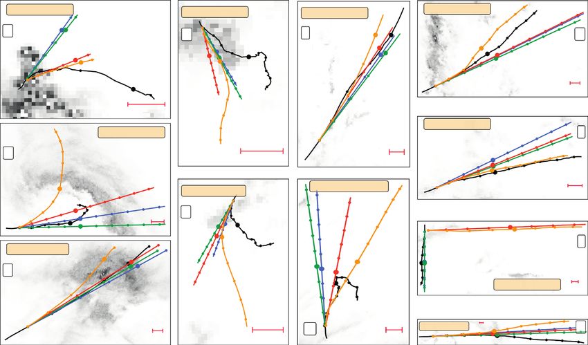
3.2. Visual Examples of Observed and Predicted Tracks. extrapolation models adequately predict the observed feature
Before we systematically evaluate the performance of dif- track varies, depending on the persistence of the motion be-
ferent extrapolation techniques, we would like to provide havior and the validity of the underlying model assumption.
some illustrative examples of observed versus predicted For example, all models perform quite well for very long times
tracks. The selection of tracks for this illustration is arbitrary in subplot (f). In subplot (i), the Semi-Lagrangian approach
and does not intend to be representative of the performance (DIS-Rot1) shows a clear advantage, while in subplots of
of any of the extrapolation methods. Instead, we aim to Figures 7(c) and 7(k), DIS-Rot1 is outperformed by all other
exemplify shapes of observed and predicted tracks under models. Surely, there are several examples (Figures 7(b), 7(d),
different sinuosity conditions in order to convey a better 7(e), and 7(g)) in which all models entirely fail to anticipate the
understanding of the various constellations that will finally motion for lead times beyond 120 minutes.
be condensed into one single location error value. As this compilation of examples is deliberately arbitrary,
Figure 7 shows a “gallery” of 11 observed tracks in it does not provide a basis to infer the general superiority or
different subplots (From Figure 7(a) to 7(k)). Each subplot inferiority of one or the other method. All models appear to
also contains the tracks that were predicted by the different struggle with predicting very sinuous tracks (subplots in
extrapolation models. Each dot represents one feature Figures 7(b), 7(d), 7(e), and 7(g)), which is what we would
location in a 30-minute time step, except the first one that expect. However, while the figure makes it difficult to
represents the first prediction step at five-minute lead time. compare the absolute location error between the examples
LK-Lin1 and LK-Lin4 infer the displacement vector di- (due to the different scales), it still appears that the absolute
rectly from the feature positions at t and t − 1 or t and t − 4, location error does not necessarily depend on the sinuosity.
respectively. As a reminder, DIS-Lin1 and DIS-Rot1 obtain For example, the location error of LK-Lin1 after the max-
the displacement vector of a feature from the DIS algo- imum lead time (280 minutes) is higher in subplot 7(i)
rithm, a dense optical flow technique that produces motion (almost straight, SI � 1.01) than it is in subplot 7(d)
fields based on the radar images at t and t − 1; DIS-Lin1 (SI � 1.36). In fact, straight tracks can imply a large error if
extrapolates the closest vector linearly over the entire lead the initial motion vector of a forecast method fails to rep-
time, while DIS-Rot1 uses a Semi-Lagrangian scheme in resent the average long-term direction (see subplot 7(j) for a
which the displacement vector is updated as the feature very impressive example). Then again, large errors can occur
moves through the velocity field obtained from the DIS if a strong sinuosity of the track coincides with a large
technique. Further details have been provided in Section overestimation of the absolute velocity (e.g., subplots 7(b)
2.3. As in all forecasts of our verification experiment, the and 7(g)). In that case, the linear extrapolation quickly
forecast time t corresponds to the 5th feature of the ob- departs from the track origin, while the actual feature track
served track. That is because the LK-Lin4 method needs to meanders slowly and remains in the close vicinity of the
look four steps back in time (t − 4) in order to produce a origin. For such a scenario, the trivial persistence model (the
forecast, while the other methods only look back one step in feature just remains at the origin) will be superior even for
time (t − 1). short lead times.8 Advances in Meteorology
Sl = 1.12 τ = 175 Sl = 1.36 τ = 300 Sl = 1.01 τ = 300
Sl = 1.01 τ = 165
(a) (d) (f) (h)
10 km
10km
Sl = 1.01 τ = 300
Sl = 1.33 τ = 300 (i)
(b)
10km 10 km
Sl = 2.22 τ = 300
Sl = 1.36 τ = 300 10 km
(e)
10km
(j)
Sl = 1.0 τ = 170
(c)
Sl = 1.01 τ = 245
10 km
(g) Sl = 1.0 τ = 300 10 km (k)
10km 10 km 10 km
0 5 10 15 20 25 30
mm/h
Observation DIS-Lin1
LK-Lin1 DIS-Rot1
LK-Lin4
Figure 7: Compilation of forecast versus observed tracks under different sinuosity conditions. Due to the different spatial extents of the
windows, the scale of each subplot is different. Hence, a 10 km scale bar is provided for orientation. For each example, the observed track
duration τ (in hours) and its sinuosity index SI are shown. The lead time of 120 minutes is highlighted by a larger dot. Some very long tracks
have been capped at a maximum of 300 minutes for illustrative purposes.
Altogether, these different examples give us a better idea all models, dramatically lower than that for the persistence
of how location errors can develop from both inadequate model; the mean error of persistence is higher than the mean
model assumptions (e.g., linear approximation versus error of any model at any lead time, which means that all
curved or sinuous conditions) and a failure to approximate models, on average, have positive skill at all lead times. For all
the average motion from the initial feature locations. It is models, the error distribution is obviously positively skewed,
impossible, though, to diagnose the superiority of one or the with the mean error being much higher than the median, and
other model from these examples. Hence, we will now thus there is a heavy tail towards high location errors.
systematically examine the results of our model verification For very short lead times of up to 10 minutes, the mean
experiment. We will not only analyze how the location error error is about one kilometer for all competing models except
depends on lead time, but we will also investigate how the for persistence which is already up at more than seven ki-
model performance relative to the persistence model de- lometers after ten minutes. After 60 minutes, the mean
pends on the sinuosity of the underlying tracks. location error of all models exceeds a distance of 5 kilo-
meters, as well as 10 kilometers after 110 minutes. For all
models, at least 25% of all forecasts exceed an error of 5
3.3. Systematic Quantification of the Location Error. After kilometers after 50 minutes and an error of 10 kilometers
having exemplified different observed and predicted tracks in after 90 minutes. After 75 minutes, at least 5% of all forecasts
the previous section, we now present the results of our exceed an error of 15 kilometers.
benchmarking experiment. Figure 8 shows the distribution of Altogether, the location error can be substantial for a
locations errors for different models and lead times up to 120 significant proportion of forecasts, while the median loca-
minutes. For each lead time, the box plots specify mean, tion error grows at a more moderate rate.
median, interquartile range, and the 5th and 95th percentiles While this general pattern governs the behavior of all
of the location error. For all models, the error quantiles in- models, there are clear differences between the performances
crease slightly exponentially but almost linearly with lead time. of the competing models. These differences, however, are not
The rate at which the location error grows with lead time is, for always coherent across all error quantiles and lead times,Advances in Meteorology 9
30
25
Median Mean
25% 95%
20
5% 75%
Distance (km)
15
10
5
0
5 10 15 20 25 30 35 40 45 50 55 60 65 70 75 80 85 90 95 100 105 110 115 120
Lead time (min)
Lk-Lin1 DIS-Rot1
Lk-Lin4 Persist
DIS-Lin1
Figure 8: The distribution of location errors for different extrapolation models and lead times.
except for the DIS-Rot1 model, which has the weakest per- examine the skill of our models more closely. Skill scores rate
formance of all models at virtually all lead times and for all the score of a forecast in relation to the score of a reference
quantiles, and the LK-Lin1 model, which performs better than forecast, in our case persistence. They are particularly useful in
DIS-Rot1 but ranks second last. As for the best forecast benchmark studies such as the present one. Equation (1)
performance, the LK-Lin4 and the DIS-Lin1 models take turns shows the general definition of skill as derived from any
depending on error quantile and lead time: For the 5th and the forecast score, as well as the specific formula if we use the
25th percentiles, the LK-Lin4 model performs best for lead location error ε as the “score” (which becomes zero for a
times up to 100 minutes, for the median up to 80 minutes, and perfect forecast) and persistence as the “reference”:
for the mean up to 55 minutes. The DIS-Lin1 model shows the
strongest changes of relative performance over lead time: as for Scoreforecast − Scorereference εforecast − εpersistence
Skill � � .
the mean error, DIS-Lin1 starts to outperform LK-Lin4 at a Scoreperfect − Scorereference −εpersistence
lead time of 60 minutes and continues this way until the (1)
maximum lead time of 120 minutes. As for the median error,
DIS-Lin1 only catches up with LK-Lin4 after 90 minutes. For We examine the forecast skill under different sinuosity
the 75th percentile, DIS-Lin1 outperforms LK-Lin4 after 50 conditions. As already pointed out in Section 3.1, the dis-
minutes and for the 95th percentile already after 20 minutes. tribution of sinuosity is highly skewed and 90% of observed
In summary, LK-Lin4 tends to outperform DIS-Lin1 in the tracks would pass as at least “rather straight” with a sinuosity
first hour, while DIS-Lin1 becomes superior in the second index equal to or lower than 1.1. Hence, we split the forecasts
hour, apparently because it tends to avoid very high errors into three unequal groups, depending on quantiles of the
more efficiently than LK-Lin4 does. sinuosity index: The first group contains the “straight” 90%
In the following, we would like to better understand how of the forecasts with a sinuosity index below 1.1. We consider
model skill is affected by sinuosity. In Section 3.2, we have the value of 1.1 as an—admittedly—arbitrary threshold
already indicated that the absolute values of location errors between “rather straight” and “rather winding” tracks. The
do not clearly depend on sinuosity. That was confirmed by remaining 10% of tracks are split into two equally sized
the systematic verification experiment (results not shown). groups, again based on sinuosity: the 5% with the highest
Yet, the difference between an extrapolation model and the sinuosity, exceeding an SI value of 1.2, could be labelled as
(trivial) persistence model might very well depend on sin- “twisted,” and the remaining 5% with intermediate SI values
uosity. In order to formally evaluate that hypothesis, we now between 1.1 and 1.2 could be labelled as “winding.” Figure 910 Advances in Meteorology
Straight : Sl < 1.1 Winding : 1.1 ≤ Sl < 1.2 Twisted : Sl ≥ 1.2
0.88 0.66 0.5
0.64
0.86 0.4
0.62
0.3
0.84 0.60
Skill
0.58 0.2
Skill
Skill
0.82 0.56
0.1
0.54
0.80
0.0
0.52
0.78 0.50 –0.1
5 30 60 90 120 5 30 60 90 120 5 30 60 90 120
Lead time (min) Lead time (min) Lead time (min)
Lk-Lin1 DIS-Lin1 Lk-Lin1 DIS-Lin1 Lk-Lin1 DIS-Lin1
Lk-Lin4 DIS-Rot1 Lk-Lin4 DIS-Rot1 Lk-Lin4 DIS-Rot1
Figure 9: The mean model skill over each lead time with regard to location prediction for different extrapolation models and sinuosity
conditions. Please note that the very low skill values of the DIS-based models at 5-minute lead time (in the winding and twisted groups) are
hidden by the scaling of the y-axis. At five-minute lead time, both models only have a skill of about 0.35 (winding) and −0.55 (twisted).
shows the average model’s skill over every lead time for these images. In our study, we detected features by using the
three sinuosity classes. Clearly, the model skill dramatically approach of Shi and Tomasi (1994) and tracked these fea-
varies between these three groups: it ranges between 0.79 tures following the approach of Lucas and Kanade [9], using
and 0.87 for the “straight” category, mostly between 0.5 and both algorithms as implemented in the OpenCV library. We
0.65 for the “winding” category, and mostly between 0 and increased the robustness of extracted feature tracks by
0.5 for the “twisted” category. This decrease of skill with making sure that the features can be successfully tracked
increasing sinuosity is well in line with our expectation. forwards and backwards. That approach, together with a
Furthermore, the ranking of all models based on skill is quite rather strict definition of parameter values for feature de-
coherent across all categories and also consistent with our tection and tracking, increases our confidence in the reli-
previous analysis of location errors. DIS-Lin1 becomes ability of the detected tracks. Still, we have to assume that the
superior within the second forecast hour, while LK-Lin1 feature locations themselves are, as any measurement, un-
performs better in the first forecast hour. Only in the certain. We expect the main sources of uncertainty to be the
“twisted” category do LK-Lin1 and, even more, LK-Lin4 grid resolution (which does not allow resolving errors below
outperform DIS-Lin1 across all lead times. It should be 1 km), and complex small-scale intensity dynamics that can
noted, though, that the overall skill in the twisted category is interfere with motion patterns. For future studies, we suggest
very low for all competing models. In the “winding” cate- a comprehensive sensitivity analysis with regard to the
gory, LK-Lin1 slightly outperforms LK-Lin4 in the first 20 parameters of the feature detection and tracking algorithms
minutes. Finally, DIS-Rot1 performs worst at all lead times in order to better understand the effects on both the number
in all categories. and the robustness of detected tracks in the context of
The change of model skill with lead time should be rainfall motion analysis. Still, we assume that the error of
interpreted with care, as it depends on both the performance extrapolating feature motion is substantially larger than the
of the extrapolation model itself and the location error of the error of feature tracking itself. In summary, we consider it
persistence model. For most models and SI categories, the warranted to use the observed tracks as a reference in order
skill appears to reach an optimum at some lead time, which to evaluate the performance (or, inversely, the error) of any
implies that the superiority of the model over persistence model that aims to predict the future locations of such
reaches a maximum. precipitation features. For that purpose, we defined the
location error of a forecast at any lead time Δt ahead of the
4. Conclusions forecast time t as the Euclidean distance between the ob-
served and the predicted feature locations at t + Δt.
In this paper, we have introduced a framework to isolate and One might want to use this approach to comprehensively
quantify the location error in precipitation nowcasts that are quantify the location error of any forecast model for the full
based on field-tracking techniques. While it is often assumed spatial domain of a forecast grid, for example, a national
that errors in precipitation nowcasts are dominated by the radar composite. In such a case, we would need to assume
temporal dynamics of precipitation intensity, the location that the average of forecast errors that we have quantified
error of predicted precipitation features has so far not been from observed feature locations in a forecast domain is
explicitly and formally quantified. representative for the average error of all location predic-
The main idea of our framework is to detect and track tions in that domain. We have not yet investigated the
scale-invariant precipitation features (corners) in radar validity of that assumption. One might argue that theAdvances in Meteorology 11
behavior of locations identified as “corners” or “good fea- precipitation nowcasting, for example, in the context of early
tures to track” might not be representative for the motion warning systems for pluvial floods in urban environments (see
behavior of the entire precipitation field; however, it will be [19]), it becomes obvious that location errors matter: the order
difficult to find evidence to either verify or falsify such a of magnitude of these errors is about the same as the typical
hypothesis, as it would require another independent way to extent of a convective cell or of a medium-sized city. Hence, the
quantify the location error. Still, we are convinced that the uncertainty of precipitation nowcasts at such length sca-
proposed framework is useful: even without the need of les—just as a result of locational errors—can be substantial
strong assumptions on representativeness, the framework already at lead times of less than an hour.
allows us to compare and benchmark the ability of different While similar conclusions have already been drawn by
models to forecast future locations of precipitation features using spatially sensitive verification measures such as the
and thus to specifically focus on improving that ability by Fractions Skill Score (see, e.g., [6]), our framework allows us to
future model development. isolate the location error for specific models and situations, to
The hypothesis that such further model developments better understand the factors that govern these errors, and
are urgently required is supported by the results of our hence to use that knowledge in order to specifically improve the
benchmarking study. It should be clarified again that this extrapolation of motion patterns in existing nowcasting models.
benchmark study does not intend to suggest better ex- As an example, we have demonstrated how the use of the
trapolation models but to demonstrate the ability of our sinuosity index can help us to better understand the predictive
framework to unravel the location errors that are produced skill and hence the uncertainty of our models in specific sit-
by state-of-the-art extrapolation methods. For that purpose, uations. We hope that the large number of extracted tracks will
we compared four models: two models use the feature lo- help to foster the development of new techniques that use data-
cations before and at forecast time t in order to derive driven machine learning models for the extrapolation of feature
displacement vectors which are then used to linearly ex- location. For that purpose, we have made openly available the
trapolate feature movement over the lead time. Model LK- full set of extracted feature tracks for the year 2016 (https://doi.
Lin1 uses the feature locations at t and t − 1, and LK-Lin4 org/10.5281/zenodo.4024272 [20]) to serve as input to future
uses the feature locations at t and t − 4. The other two models studies. However, such future studies should also use radar data
are based on the dense optical flow algorithm DIS that from a longer time period in order to learn more about the
generates a full motion vector field under various seasonal effects related to the properties of feature tracks.
smoothness constraints. The model DIS-Lin1 obtains the
displacement vector for a feature at t from the nearest Data Availability
motion vector in the field based on the radar images at times
The radar data are provided by DWD at https://opendata.
t and t − 1 and uses that vector over the entire lead time. DIS-
dwd.de/weather/radar/radolan/ry (last access: Sept. 2020).
Rot1, in contrast, uses a Semi-Lagrangian scheme in which
The code of this analysis is available in the Github repository
the displacement vector is updated as the feature moves
under https://github.com/arthurcts/loc_error (last access:
through the motion field obtained from the DIS technique.
Sept. 2020). The dataset of extracted feature tracks has been
The motivation behind the DIS-Rot1 model is to better
deposited in the Zenodo repository (https://doi.org/10.5281/
represent rotational or curved motion patterns. From these
zenodo.4024272).
four competing models, LK-Lin4 appears to be the best
model in the first forecast hour and DIS-Lin1 the best in the Conflicts of Interest
second. DIS-Rot1 performs consistently the worst. That is
not quite in line with our naive expectation in which we The authors declare that there are no conflicts of interest
would hope that a Semi-Lagrangian approach should be able regarding the publication of this paper.
to better capture at least curved motion patterns. But not
even in the winding category does the complexity of the DIS- Acknowledgments
Rot1 approach pay off. Whether that is due to the imple-
mentation of the Semi-Lagrangian approach or due to the The authors acknowledge the German Weather Service,
lack of validity of the approach should be the subject of namely, Dr. Tanja Winterrath, for making the RY data
future research. Comparing LK-Lin1 to LK-Lin4, we see a available from the latest RADKLIM reanalysis. Arthur Costa
clear advantage in looking back in time more than one step. Tomaz de Souza has been funded by a Ph.D. scholarship of
It appears that, this way, we can retrieve more reliable, more the German Academic Exchange Service (DAAD). Georgy
representative, and less noisy displacement vectors, which Ayzel was partly funded by the ClimXtreme project (BMBF,
shows in the superiority of LK-Lin4 over LK-Lin1. FKZ 01LP1903B).
For all competing models, the mean location error exceeds
a distance of 5 kilometers after 60 minutes and 10 kilometers References
after 110 minutes. At least 25% of all forecasts exceed an error
[1] M. Reyniers, Quantitative Precipitation Forecasts Based on
of 5 kilometers after 50 minutes and an error of 10 kilometers Radar Observations: Principles, Algorithms and Operational
after 90 minutes. Even for the best models in our experiment, at Systems, Institut Royal Météorologique de Belgique, Brussel,
least 5 percent of the forecasts will have a location error of more Belgium, 2008.
than 10 kilometers after 45 minutes. When we relate such [2] G. Ayzel, M. Heistermann, and T. Winterrath, “Optical flow
errors to application scenarios that are typically suggested for models as an open benchmark for radar-based precipitation12 Advances in Meteorology
nowcasting (rainymotion v0. 1),” Geoscientific Model Develop-
ment, vol. 12, pp. 1387–1402, 2019.
[3] C. Pierce, A. Seed, S. Ballard, D. Simonin, and Z. Li, “Nowcasting,”
in Doppler Radar Observations—Weather Radar, Wind Profiler,
Ionospheric Radar, and Other Advanced Applications, J. Bech, Ed.,
InTech, London, UK, 2012, http://www.intechopen.com/books/
doppler-radar-observations-weather-radar-wind-profiler-ionosp
heric-radar-and-other-advanced-applications/nowcasting.
[4] M. E. Baldwin and J. S. Kain, “Sensitivity of several performance
measures to displacement error, bias, and event frequency,”
Weather and Forecasting, vol. 21, no. 4, pp. 636–648, 2006.
[5] E. E. Ebert, “Fuzzy verification of high-resolution gridded fore-
casts: a review and proposed framework,” Meteorological Appli-
cations, vol. 15, no. 1, pp. 51–64, 2008.
[6] G. Ayzel, T. Scheffer, and M. Heistermann, “RainNet v1.0: a
convolutional neural network for radar-based precipitation
nowcasting,” Geoscientific Model Development, vol. 13, no. 6,
pp. 2631–2644, 2020.
[7] C. Schmid, R. Mohr, and C. Bauckhage, “Evaluation of interest
point detectors,” International Journal of Computer Vision, vol. 37,
no. 2, pp. 151–172, 2000.
[8] J. Shi and C. Tomasi, “Good features to track,” in Proceedings of
the 9th IEEE Conference on Computer Vision and Pattern
Recognition, Springer, Seattle, WA, USA, 1994.
[9] B. D. Lucas and T. Kanade, “An iterative image registration
technique with an application to stereo vision,” in Proceedings
of the 7th International Joint Conference on Artificial Intel-
ligence, p. 674, Vancouver, BC, Canada, August 1981.
[10] J. Y. Bouguet, “Pyramidal implementation of the Lucas
Kanade feature tracker description of the algorithm,” Tech-
nical report, Intel Corporation, Microprocessor Research
Labs, Santa Clara, CA, USA, 2000.
[11] OpenCV library, “OpenCV: optical flow,” 2020, https://docs.
opencv.org/4.4.0/d4/dee/tutorial_optical_flow.html.
[12] J. E. Mueller, “An introduction to the hydraulic and topo-
graphic sinuosity Indexes1,” Annals of the Association of
American Geographers, vol. 58, no. 2, pp. 371–385, 1968.
[13] J. P. Terry and C.-C. Feng, “On quantifying the sinuosity of
typhoon tracks in the western North Pacific basin,” Applied
Geography, vol. 30, no. 4, pp. 678–686, 2010.
[14] OpenCV library, “OpenCV: DISOpticalFlow class reference,”
2020, https://docs.opencv.org/4.4.0/de/d4f/classcv_1_1DISO
pticalFlow.html.
[15] T. Kroeger, R. Timofte, D. Dai, and L. Van Gool, “Fast optical
flow using dense inverse search,” in Proceedings of the Eu-
ropean Conference on Computer Vision, Amsterdam, The
Netherlands, Springer, October 2016.
[16] U. Germann and I. Zawadzki, “Scale-dependence of the pre-
dictability of precipitation from continental radar images. Part I:
description of the methodology,” Monthly Weather Review,
vol. 130, no. 12, pp. 2859–2873, 2002.
[17] T. Winterrath, “Erstellung einer radargestützten nieders-
chlagsklimatologie (creation of a radar-based precipitation cli-
matology),” Berichte des Deutschen Wetterdienstes, Deutscher
Wetterdienst, Offenbach, Germany, 2017, https://www.dwd.de/
DE/leistungen/pbfb_verlag_berichte/pdf_einzelbaende/251_pdf.
pdf.
[18] DWD, “German climate Atlas,” 2020, https://www.dwd.de/EN/
ourservices/germanclimateatlas/germanclimateatlas.html.
[19] A. Zanchetta and P. Coulibaly, “Recent advances in real-time
pluvial flash flood forecasting,” Water, vol. 12, no. 2, p. 570, 2020.
[20] A. C. T. Souza, “Set of extracted feature tracks for the year
2016,” Zenodo, 2020.You can also read


