Prediction performance of space weather forecast centers following the extreme events of October and November 2003
←
→
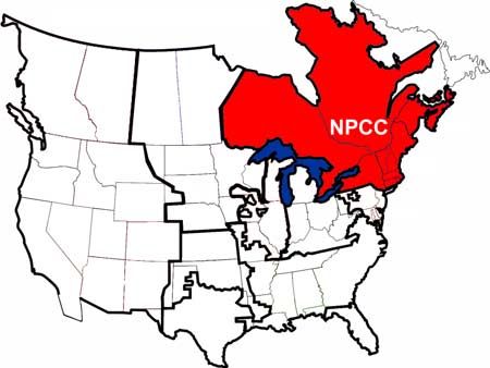
Page content transcription
If your browser does not render page correctly, please read the page content below
SPACE WEATHER, VOL. 2, S08001, doi:10.1029/2004SW000076, 2004

Prediction performance of space weather forecast centers
following the extreme events of October
and November 2003
Cary Oler
Solar Terrestrial Dispatch, Stirling, Alberta, Canada
Received 25 February 2004; revised 16 April 2004; accepted 28 April 2004; published 5 August 2004.

[1] A review and analysis of the five strongest interplanetary coronal mass ejection (ICME)
events of late October and early November 2003 (the strongest events of the ‘‘Halloween’’ epoch)
are studied with respect to the prediction performance of five space weather forecast centers.
Accurate time-of-arrival predictions and rapid responses to the upstream detection of strong
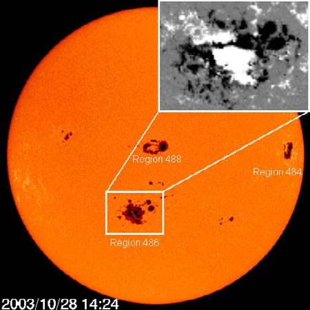
ICMEs are of paramount importance to critical infrastructures such as power companies.
Prediction and performance analysis results indicate that (1) the average time-of-arrival error for
all forecast centers was 9.26 hours, which is consistent with the guidance errors associated with
the leading shock propagation prediction models; (2) time-of-arrival predictions from Solar
Terrestrial Dispatch (STD) surpassed all others in accuracy, with an average time-of-arrival
prediction error of 1.22 hours; (3) overall, the strongest ICME impact events of 29 and 30 October
were the most poorly predicted; (4) the most accurate shock propagation prediction model
operated by the Geophysical Institute of the University of Alaska Fairbanks was the HAFv.2
model; and (5) STD provided the most rapid notification to the Northeast Power Coordinating
Council concerning the detection and imminent arrival of most of the ICMEs. A better method
of conveying time-of-arrival prediction information is presented that may be more easily
digested by consumers of space weather services.          INDEX TERMS: 2722 Magnetospheric Physics:
Forecasting; 2788 Magnetospheric Physics: Storms and substorms; 2409 Ionosphere: Current systems (2708); 2139
Interplanetary Physics: Interplanetary shocks; KEYWORDS: prediction, GIC, Halloween, performance, storm, CME
Citation: Oler, C. (2004), Prediction performance of space weather forecast centers following the extreme events of October
and November 2003, Space Weather, 2, S08001, doi:10.1029/2004SW000076.

1. Introduction                                                          [4] Whether a high-velocity ICME succeeds in producing
  [2] Significant solar activity can have strong impacts on            an intense geomagnetic storm depends on the presence of
technology and infrastructure systems [Lambour et al., 2003].          strong southward magnetic fields imbedded within the
The severe geomagnetic storm and associated province-                  sheath region [Tsurutani et al., 1988; Gosling and McComas,
wide power blackout in Quebec on 13 and 14 March 1989                  1987] and/or the core (e.g., the magnetic cloud) of the ICME
[Czech et al., 1992] forms the historical basis for illustrating       [Gonzalez et al., 1998]. The arrival of these fields at the Earth
the deleterious effects of strong space weather activity on            can produce strong magnetospheric current systems
critical infrastructure systems such as those in the North-            minutes to hours after the initial impact of the ICME shock
east Power Coordinating Council (NPCC) region (Figure 1),              front (depending on where in the ICME the southward
which has been historically sensitive to space weather                 fields reside). Thus, although the time of arrival of an ICME
storms and geomagnetically induced currents (GICs).                    is not by itself sufficient to predict magnetic storm effects, it
  [3] It is now widely recognized that most intense geo-               is sufficient to predict when strong ICMEs may first begin
magnetic storms are caused by high-velocity coronal mass               impacting vulnerable industries such as power grids. For
ejections [Tsurutani et al., 1988; Gosling et al., 1991; Richardson    example, the initial shock-driven impact of ICMEs can
et al., 2001; Yurchyshyn et al., 2004] associated with extended        produce sudden magnetic impulses [Siscoe et al., 1968;
periods (several hours) of strong southward (less than                 Ogilvie et al., 1968; Araki, 1977; Gosling et al., 1991; Russell et
  10 nT) interplanetary magnetic fields (IMFs) [Gonzalez               al., 1994] that can drive ground-induced currents through
and Tsurutani, 1987; Gonzalez et al., 1994]. The strength of           power grids around the world nearly simultaneously. These
the IMF, and to a lesser but still notable degree the strength         are reasons why power (and other) industries vulnerable to
of the southward component, has been correlated                        space weather are heavily concerned with the accurate
with interplanetary coronal mass ejection (ICME) velocity              prediction of the arrival time of significant ICME distur-
[Gonzalez et al., 1998; Lindsay et al., 1999; Yurchyshyn et al.,       bances. This study therefore concentrates on the shock
2004]. Thus high-velocity Earthward directed ICMEs have                time-of-arrival predictions of the 24 October to 4 November
the greatest potential to produce the strongest geomagnetic            events as a significant indicator of space weather forecast
storms.                                                                center prediction performance.

Copyright 2004 by the American Geophysical Union                S08001                                                            1 of 12
S08001              OLER: PREDICTION PERFORMANCE DURING EXTREME SPACE WEATHER                                        S08001

                                                                predictions from this group of researchers will hereinafter
                                                                be referred to as the GI predictions.
                                                                  [11] 5. Solar Influences Data Center (SIDC): A regional
                                                                warning center in Belgium for the European region pro-
                                                                duces predictions that are distributed to recipients through
                                                                e-mail distribution lists and also publicly through its Web
                                                                site (sidc.oma.be).
                                                                  [12] 6. Geological Survey of Canada (GSC): A regional
                                                                warning center distributes prediction information via a
                                                                publicly accessible Web site (www.spaceweather.gc.ca). It
                                                                is also a secondary source of prediction information for the
                                                                NPCC. Unfortunately, documented time-of-arrival predic-
                                                                tions do not appear to have been produced. As a result, the
                                                                GSC has been excluded from the bulk of this study.
                                                                  [13] 7. Metatech Corporation (MC): A commercial space
                                                                weather provider for a power company in the United
   Figure 1. Domain of the NPCC control regions.
                                                                Kingdom provides publicly available space weather
                                                                advisories through its Web site (www.metatechcorp.com).
                                                                Unfortunately, MC advisory notices during this period did
  [5] To be included in this study, a forecast center must      not contain sufficient information or were too ambiguous
have provided prediction information for each of the five       to determine specific time-of-arrival prediction dates for
strongest ICME events of this epoch. In addition, each          many of the events studied. The predictions from MC are
prediction must have been time or date stamped and              therefore not suitable for inclusion in this study.
placed in the public domain prior to the arrival of the           [14] The first five space weather forecast centers enu-
ICMEs. Suitable prediction distribution methods include         merated above provided suitable prediction information to
e-mail distribution lists and publicly accessible Web pages.    be included in this study. This study does not discuss the
  [6] For this study, the predictions from the follow-          observed effects of the storm activity of October and
ing space weather forecast centers were examined for            November on the power grids in the NPCC region. A
suitability.                                                    separate paper is being prepared for publication that will
  [7] 1. Space Environment Center (SEC): The world              address those impacts.
warning space weather agency distributes prediction in-           [15] A brief examination of the solar drivers responsible
formation via e-mail distribution lists as well as a publicly   for the strong ICME events of this epoch is presented in
accessible Web site (www.sec.noaa.gov). SEC is also a           section 2. The time-of-arrival predictions of each forecast
secondary source of prediction information for the NPCC.        center are then examined along with the best and worst
  [8] 2. Solar Terrestrial Dispatch (STD): The primary          predictions in section 3. In section 4 we examine the
space weather forecast center for the NPCC region dis-          maximum lead time performance of STD, SEC, and IPS
tributes prediction information via e-mail distribution lists   (where STD and SEC rendered services directly to the
as well as a publicly accessible Web site (www.spacew.          NPCC). In section 5 we introduce the use of impact
com).                                                           prediction windows and discuss their usefulness to space
  [9] 3. Ionospheric Prediction Service (IPS) Radio and         weather consumers.
Space Services: A regional warning center in Australia
distributes prediction information via e-mail distribution
                                                                2. Solar Sources of the Extreme Events
lists as well as a publicly accessible Web site (www.ips.
gov.au).
                                                                of October and November 2003
  [10] 4. Geophysical Institute (GI) of the University of         [16] Solar activity intensified to high levels from mid-
Alaska Fairbanks and Exploration Physics International:         October through early November 2003 following the emer-
The research group associated with these organizations          gence of three very large and active sunspot groups
produces unofficial ‘‘fearless forecasts’’ jointly with Space   (Figure 2). Between 19 October and 4 November these
Environment Center (SEC)/National Oceanic and Atmo-             groups were associated with some of the most intense
spheric Administration researchers that are based on the        solar activity on record. X-ray flare emissions broke long-
results of evolving kinematic and semiempirical models of       standing records. The geomagnetic storms of 29 and
solar wind flows. This group is not an official ‘‘forecast      30 October were the most intense of solar cycle 23 and
center’’ but rather a research group working on improving       were ranked 6th and 16th, respectively, on the ‘‘Top 30’’
the performance and operational parameters of several           list assembled by SEC for the events commencing from
prominent shock propagation models. Their predictions           1936 (SEC Power Point presentation, ‘‘Post event review
are designed to be objective with minimal bias. They            for October 19th -- November 17th events,’’ 21 November
distribute their predictions through an e-mail distribution     2003, hereinafter referred to as SEC, 2003). The intensity
list, and the results of their predictions are also publicly    and frequency of the solar X-ray activity are illustrated in
available through their Web site (gse.gi.alaska.edu). The       the plot of Figure 3.

                                                                                                                     2 of 12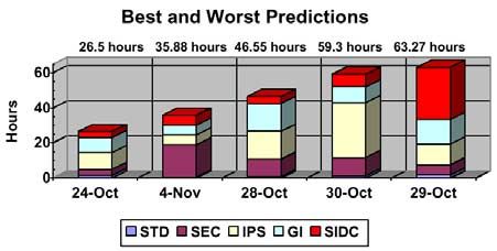
S08001              OLER: PREDICTION PERFORMANCE DURING EXTREME SPACE WEATHER                                     S08001

                                                              complex formed and maintained a strong magnetic
                                                              delta configuration throughout its passage across the
                                                              solar disk and unleashed several additional strong solar
                                                              flares.
                                                                [18] Region 10486 (or 486) rotated into view around
                                                              the southeastern solar limb on 22 October. This region
                                                              matured as it rotated toward the central solar meridian
                                                              and quickly asserted itself as the most prolific flare
                                                              producer of the trio of large spot groups. Multiple mag-
                                                              netic delta configurations were evident in this region (see
                                                              Figure 2) that supported the eruption of multiple intense
                                                              X-class solar flares.
                                                                [19] Region 10488 (or 488) emerged on the visible disk
                                                              north and slightly west of region 486 on 27 October. How-
                                                              ever, it remained comparatively quiet until it approached
                                                              the western solar limb and did not produce any significant
                                                              ICMEs.
                                                                [20] During the period of 22 October to 4 November,
                                                              there were nine strong partial and/or full halo coronal
                                                              mass ejections determined by the Solar and Heliospheric
                                                              Observatory (SOHO) spacecraft science team. Eight of
Figure 2. Map of active regions just after the large          these events were determined as ‘‘front-sided.’’ Total
X17/4B proton flare of 28 October and the associated          magnetic field data from the Advanced Composition Ex-
geoeffective ICME from region 486. Images courtesy of         plorer (ACE) satellite shows eight relatively well defined
Solar and Heliospheric Observatory Michelson Dop-             transient disturbances in the solar wind during this same
pler Imager.                                                  time interval (see Figure 4).
                                                                [21] Solar wind velocity, density, and temperature data
                                                              were not available for several of the strongest events
  [17] Region 10484 (hereinafter referred to as region 484)   because of proton contamination of the ACE Solar Wind,
was the first influential sunspot complex to rotate into      Electron, Proton, and Alpha Monitor (SWEPAM) sensors.
view around the northeastern solar limb on 18 October         Thus only the total interplanetary magnetic field (IMF)
2003. It grew exceptionally rapidly and produced several      strength values were used to sort the ICMEs by strength.
energetic solar flares on 19 October, including the first     The five strongest and best defined ICMEs used in this
X-class flare in four months (since 15 June 2003), which      study (all events with peak IMF magnitudes above 20 nT)
was successfully (and solely) predicted a little over         are listed in Table 1, sorted according to their dates of
12 hours earlier by Solar Terrestrial Dispatch. This spot     occurrence and ranked according to IMF strength. These

         Figure 3. X-ray flare activity from 19 October through 4 November. Note the rapid ascent and
         decay of the background X-ray flux as the active regions appeared, matured, and then rotated out
         of view behind the west limb. The primary geoeffective solar events occurred between 22 October
         and 2 November.

                                                                                                                  3 of 12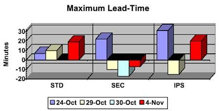
S08001              OLER: PREDICTION PERFORMANCE DURING EXTREME SPACE WEATHER                                          S08001

         Figure 4. Interplanetary magnetic field data as measured by the ACE spacecraft for the events of
         24 October through 6 November. Each event is ranked according to strength by sorting the
         observed peak total magnetic field magnitudes (Bt). Since we are primarily concerned with the
         prediction performance of the most extreme ICME events, only those events with total magnetic
         field values that peaked above 20 nT are considered in this study. The events satisfying this
         criteria are identified as events 1 --5 and are listed in Table 1.

five selected events were the only ones associated with         A map of the physical locations of each of the events in
periods of severe planetary geomagnetic storm activity          Table 1 is illustrated in Figure 6.
(planetary Kp indices of 7 -- or greater).                        [23] Note that although the most extreme coronal mass
  [22] Table 1 and Figures 5 and 6 illustrate the widely        ejection having a plane-of-sky velocity of 2381 km sec 1
varying characteristics, locations, and inferred trajectories   was observed on 4 November in association with the X28
of each of the solar driver events. The variances in the        solar flare event (as extrapolated from saturated GOES
characteristics and trajectories of the five selected events    X-ray data by SEC and more recently estimated as an
should be sufficient to reveal the skill of each forecast       X40-X50 event through its X-ray impact on the Earth’s
center in assessing and predicting their respective impacts.    ionosphere [Thomson et al., 2004]), the Earth-bound impact

Table 1. Characteristics of the Five Strongest ICMEs
                                                                                               Estimated          Estimated
                  ICME Ejection     Associated Solar      Integrated       SSC or Sudden        Type II          Plane-of-Sky
                    Date and             Event               X-Ray        Impulse at Earth   Shock Velocity,       Velocity
Event    Rank    Time (From C2)     (Type II Onset)       Flux, J m 2      Date and Time        km s 1         (SOHO), km s     1

  1       3        22 Oct. 2003       22 Oct. 2003      multiple peaks;     24 Oct. 2003          650                898
                    0745 UTC            0938 UTC          complex            1529 UTC
                                       region 484,
                                     multiple X ray,
                                         N08E19
                                                                     1
  2       5        26 Oct. 2003       26 Oct. 2003        6.3  10          28 Oct. 2003          950               1432
                    1754 UTC            1735 UTC                             0206 UTC
                                       region 484,
                                    X1.2/1N, N02W38
  3       1        28 Oct. 2003       28 Oct. 2003         1.8  100        29 Oct. 2003          1250              2125
                    1054 UTC            1102 UTC                             0613 UTC
                                       region 486,
                                    X17.2/4B, S16E08
                                                                     1
  4       2        29 Oct. 2003       29 Oct. 2003        8.7  10          30 Oct. 2003          775               1948
                    2054 UTC            2042 UTC                             1640 UTC
                                       region 486,
                                    X10.0/2B, S15W02
                                                                     1
  5       4        2 Nov. 2003        02 Nov. 2003        9.1  10          4 Nov. 2003           1691              1826
                    1730 UTC            1714 UTC                             0627 UTC
                                       region 486,
                                    X8.7/2B, S14W56

                                                                                                                       4 of 12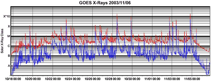
S08001             OLER: PREDICTION PERFORMANCE DURING EXTREME SPACE WEATHER                                  S08001

         Figure 5. Large Angle and Spectrometric Coronagraph (LASCO) experiment C3 images
         illustrating the relative trajectories of each of the ICMEs associated with the events in Table 1.
         The event following the X28/SEC or X40-50/Thomson flare of 4 November is also shown for
         completeness, even though the Earth-bound impact was too weak to appear on our list of the five
         strongest events. The image of 2 November does not show the full halo coronal mass ejection very
         well because of strong proton contamination of the LASCO camera. As these images suggest, the
         trajectories of these coronal mass ejection events varied significantly with primary radial
         components directed toward the Earth and at apparent near -- right angles to the Earth.

                                                                                                              5 of 12
S08001 OLER: PREDICTION PERFORMANCE DURING EXTREME SPACE WEATHER S08001
arrivals that span a portion of a UTC day. For example,
SEC’s prediction for 26 October (a copy of this report is
available from sec@sec.noaa.gov) stated
Geophysical activity forecast: the geomagnetic field is expected
to be quiet to active all three days, with possible minor storm
conditions on day two due to a partial halo CME from the X1.2
flare observed today at 0654 UTC.
[26] Thus the only useful time-of-arrival prediction in-
formation from SEC for this event is a 24-hour window
centered on ‘‘day two,’’ corresponding to the UTC day of
28 October. This is a common trait observed with most
forecast centers.
[27] The uncertainties in the time-of-arrival statements
given by SEC, IPS, and SIDC make it difficult to determine
preferred times of arrivals. For these forecasts we look at
the wording used in the predictions and take the best
reasonable estimate. For example, IPS predicted that the
disturbance of 28 October would arrive some time during
Figure 6. Probable solar source locations of the five the ‘‘2nd half of the UT day of 28 October.’’ We therefore
strongest ICME impacts. The two solar events asso- assigned this event a ‘‘most reasonable’’ time of arrival of
ciated with the strongest ICME impacts are indicated 1800 UTC, which is the midpoint of the second half of the
with circled dots. UTC day. The resulting prediction error is subject to some
uncertainty (in this case, roughly 6 hours) but should
of that event was ranked as the weakest because of the represent a reasonable estimate given the available form
poor location of the solar driver on the west limb and has of the prediction statement. Later in this study, we look at
therefore been excluded from this study. the results of adjusting the most reasonable times of
arrivals in order to minimize the errors within the con-
straints imposed by the given forecast statements.
3. Time-of-Arrival Prediction Analysis [28] The researchers associated with the GI make multi-
[24] The five space weather forecast center predictions ple objective predictions using a suite of solar wind shock
are listed in Tables 2 -- 6. Only the first official time-of- propagation models, including the shock time of arrival
arrival predictions issued by each forecast center are used (STOA) model [Dryer and Smart, 1984; Smart et al., 1984,
in order to prevent the introduction of undue bias and to 1986; Smart and Shea, 1985; Lewis and Dryer, 1987] and the
ensure as accurate a comparison as possible. revised STOA-2 model [Moon et al., 2002; Vlasov, 1988,
[25] Most forecast centers are careful when it comes to 1992], the interplanetary shock propagation model (ISPM)
specifying time-of-arrival estimates. Time-of-arrival pre- [Smith and Dryer, 1995], and the HAFv.2 model [Fry, 1985;
dictions are very difficult to accurately determine, and Fry et al., 2001; Hakamada and Akasofu, 1982].
there are always a number of hours of uncertainty. As a [29] To make use of the GI predictions in this study, it
result, most forecast centers indicate predicted times of is necessary to establish a most reasonable time-of-
Table 2. Prediction Performance of Solar Terrestrial Dispatcha
Most
Actual Reasonable Lead Time
Observed ICME Impact Issue Time of Prediction Minimized Between Alert
Impact Date Prediction Prediction Error Error K 6 or 7 Alert Date Issued and ICME Arrival
24 Oct. 2003 24 Oct. 2003 22 Oct. 2003 1 hour 1 hour 29 min 24 Oct. 2003 1522 UTC +7 min
1529 UTC 1400 UTC 1845 UTC 29 min
28 Oct. 2003 28 Oct. 2003 27 Oct. 2003 54 min 54 min none issued or required not applicable;
0206 UTC 0300 UTC 0630 UTC no alert issued
29 Oct. 2003 29 Oct. 2003 28 Oct. 2003 1 hour 1 hour 47 min 29 Oct. 2003 0603 UTC +10 min
0613 UTC 0800 UTC 1630 UTC 47 min
30 Oct. 2003 30 Oct. 2003 30 Oct. 2003 1 hour 1 hour 20 min alert in progress separate notice
1640 UTC 1800 UTC 0405 UTC 20 min continued from of shock arrival
previous event sent out at
1657 UTC
4 Nov. 2003 4 Nov. 2003 2 Nov. 2003 33 min 33 min 4 Nov. 2003 0608 UTC +19 min
0627 UTC 0700 UTC 2250 UTC
a
Average time-of-arrival prediction error was 1 hour 13 min.
6 of 12S08001 OLER: PREDICTION PERFORMANCE DURING EXTREME SPACE WEATHER S08001
Table 3. Prediction Performance of Space Environment Centera
Lead Time
Observed ICME Most Reasonable Issue Time of Prediction Minimized K 6 or 7 Alert Between Alert
Impact Date Impact Prediction Prediction Error Error Date Issued and ICME Arrival
24 Oct. 2003 24 Oct. 2003 22 Oct. 2003 3 hours 29 min 0 hours 0 min 24 Oct. 2003 +22 min
1529 UTC 1200 UTC, 2240 UTC 1507 UTC
‘‘mid-day on 24 Oct.’’
28 Oct. 2003 28 Oct. 2003 26 Oct. 2003 9 hours 54 min 0 hours 0 min none issued or not applicable
0206 UTC 1200 UTC, 2200 UTC required; no major since an alert
‘‘minor storm or severe storm was not issued
conditions was observed
on day two’’
29 Oct. 2003 29 Oct. 2003 28 Oct. 2003 5 hours 47 min 0 hours 0 min 29 Oct. 2003 10 min
0613 UTC 1200 UTC, 2200 UTC 0623 UTC
‘‘likely impact the
earth’s magnetic
field by mid-day
on day one’’
30 Oct. 2003 31 Oct. 2003 29 Oct. 2003 10 hours 20 min 7 hours 20 min 30 Oct. 2003 17 min
1640 UTC 0300 UTC, 2200 UTC 1657 UTC
‘‘impact from
today’s X10 flare
will be assessed
next period;
predictions for
days two and
three will likely
change considerably’’
4 Nov. 2003 3 Nov. 2003 2 Nov. 2003 18 hours 27 min 12 hours 27 min 4 Nov. 2003 7 min
0627 UTC 1200 UTC, 2200 UTC 0634 UTC
‘‘beginning on
day one near the
middle of the day’’
a
Average time-of-arrival prediction error was 9 hours 35 min. Impact date was obtained from ground-level magnetometer data. Impact
predictions were obtained from the daily ‘‘Report of Solar and Geophysical Activity’’ (www.sec.noaa.gov/forecast.html). K 6 or 7 alerts were
obtained in real time from SEC via e-mail and documented in its Preliminary report and forecast of Solar Geophysical Data (www.sec.noaa.gov/
weekly).
Table 4. Predictions of IPS Radio and Space Services Australiaa
Lead Time
Observed ICME Most Reasonable Prediction Prediction Minimized Storm Alert Between Alert
Impact Date Impact Prediction Issue Time Error Error Date/Time and ICME Arrival
24 Oct. 2003 24 Oct. 2003 22 Oct. 2003 9 hours 29 min 0 hours 0 min 24 Oct. 2003 +31 min
1529 UTC 0600 UTC, 2330 UTC 1458 UTC
‘‘early on 24th’’
28 Oct. 2003 28 Oct. 2003 26 Oct. 2003 15 hours 54 min 9 hours 54 min no alert issued not applicable
0206 UTC 1800 UTC, 2330 UTC or required; since an alert
‘‘2nd half of UT no major or severe was not issued
day on 28 Oct.’’ storm was observed
29 Oct. 2003 29 Oct. 2003 28 Oct. 2003 11 hours 47 min 5 hours 47 min 29 Oct. 2003 15 min
0613 UTC 1800 UTC, 2211 UTC 0628 UTC
‘‘2nd half of UT
day on 29 Oct.’’
30 Oct. 2003 01 Nov. 2003 29 Oct. 2003 31 hours 20 min 19 hours 20 min first mention excluded
1640 UTC 0000 UTC, 2330 UTC of storm on
‘‘late on 31 Oct. 30 Oct. at
or early on 01 Nov.’’ 2025 UTC
by automated
K = 7 detection
4 Nov. 2003 4 Nov. 2003 2 Nov. 2003 5 hours 33 min 0 hours 0 min 4 Nov. 2003 +20 min
0627 UTC 1200 UTC, 2330 UTC 0607 UTC
‘‘around mid-day
on 04 Nov.’’
a
Average time-of-arrival prediction error was 14 hours 49 min. Impact date was obtained from ground-level magnetometer data. Impact
predictions and issued storm alerts are available in real time via e-mail and are archived at www.ips.gov.au.
7 of 12S08001 OLER: PREDICTION PERFORMANCE DURING EXTREME SPACE WEATHER S08001
Table 5. Predictions of Geophysical Institute, University of Alaska at Fairbanksa
HAFv.2 STOA STOA-2 ISPM Selected
Observed Impact Prediction Impact Prediction Impact Prediction Impact Prediction Prediction
Impact Prediction Error Prediction Error Prediction Error Prediction Error Error
24 Oct. 25 Oct. 11 hours 24 Oct. 1 hour 24 Oct. 6 hours 25 Oct. 13 hours 8 hours
1529 UTC 0300 UTC 31 min 1331 UTC 58 min 0840 UTC 49 min 0526 UTC 57 min 34 min
28 Oct. 28 Oct. 1 hours 28 Oct. 16 hours 28 Oct. 18 hours 29 Oct. 27 hours 15 hours
0206 UTC 0400 UTC 54 min 1812 UTC 6 min 2017 UTC 11 min 0541 UTC 35 min 57 min
29 Oct. 30 Oct. 19 hours 29 Oct. 11 hours 29 Oct. 12 hours 29 Oct. 13 hours 14 hours
0613 UTC 0200 UTC 47 min 1713 UTC 0 min 1833 UTC 20 min 1936 UTC 23 min 8 min
30 Oct. 30 Oct. 3 hours 31 Oct. 10 hours 31 Oct. 19 hours 30 Oct. 2 hours 8 hours
1640 UTC 2000 UTC 20 min 0319 UTC 39 min 1141 UTC 01 min 1933 UTC 53 min 58 min
4 Nov. 04 Nov 3 hours 4 Nov. 2 hours 4 Nov. 15 hours 4 Nov. 2 hours 5 hours
0627 UTC 0300 UTC 27 min 0412 UTC 15 min 2138 UTC 11 min 0413 UTC 14 min 47 min
a
Average time-of-arrival prediction errors were 8 hours 0 min (HAFv.2), 8 hours 24 min (STOA), 14 hours 18 min (STOA-2), and 12 hours
0 min (ISPM). Overall average prediction error was 10 hours 41 min.
arrival prediction based on the suite of predictions [31] Unfortunately, the ICME from this event arrived
issued for each event. This was done by selecting the before SEC’s ‘‘next period.’’ We are therefore left with
average of the four published time-of-arrival predictions only the last snippet of this statement for clues as to when
for STOA, STOA-2, ISPM, and HAFv.2, (shown in the the forecaster thought the disturbance might arrive. These
‘‘selected’’ column of Table 5). Earlier studies of these snippets suggest that the SEC forecaster believed that the
models have shown that time-of-arrival errors of be- ICME would impact on days 2 and 3 (31 October and
tween 9.8 and 11.6 hours are to be expected [Cho et al., 1 November). We have therefore assigned an impact time
2003]. Our most reasonable average error of 10.68 hours of 0300 UTC on 31 October as an estimate, reasoning that
for the suite of models is therefore in good agreement the forecaster would have preferred an early UTC day
with these findings. impact on 31 October.
[30] The most uncertain prediction for which a preferred
time of arrival was difficult to determine was issued by the 3.1. Time-of-Arrival Prediction Results
Space Environment Center on 29 October. Its daily sum- [32] Figure 7 provides a side-by-side comparison of the
mary report (a copy is available from sec@sec.noaa.gov) most reasonable time-of-arrival predictions for each of the
stated that forecast centers and for the five strongest space weather
The potential geomagnetic impact from today’s X10 flare will events of 24 October through 4 November. Clearly, the
be assessed next period; predictions for days two and three predictions from STD were associated with the lowest
will likely change considerably. prediction errors.
Table 6. Solar Influences Data Center (SIDC) Belgium Predictionsa
Observed ICME Most Reasonable Prediction Prediction Minimized
Impact Date Impact Prediction Issue Time Error Error
24 Oct. 2003 24 Oct. 2003 23 Oct. 2003 1333 UTC 3 hours 29 min 0 hours 0 min
1529 UTC 1200 UTC,
‘‘to become
geoeffective
by 24 Oct.’’
28 Oct. 2003 28 Oct. 2003 27 Oct. 2003 1230 UTC 3 hours 54 min 0 hours 0 min
0206 UTC 0600 UTC,
‘‘early on 28 Oct.’’
29 Oct. 2003 30 Oct. 2003 28 Oct. 2003 1230 UTC 29 hours 47 min 17 hours 47 min
0613 UTC 1200 UTC,
‘‘major to severe
magnetic storm on
Thursday 30 Oct.’’
30 Oct. 2003 31 Oct. 2003 30 Oct. 2003 1351 UTC 7 hours 20 min 1 hour 20 min
1640 UTC 0000 UTC,
‘‘tonight or early
tomorrow (31Oct.)’’
4 Nov. 2003 4 Nov. 2003 3 Nov. 2003, 1227 UTC 5 hours 33 min 0 hours 0 min
0627 UTC 1200 UTC,
‘‘may arrive on
04 November’’
a
Average time-of-arrival prediction error was 10 hours 1 min. Impact date was obtained from ground-level magnetometer
data. Impact predictions are available via e-mail and at www.sidc.oma.be.
8 of 12S08001 OLER: PREDICTION PERFORMANCE DURING EXTREME SPACE WEATHER S08001
Figure 9. Cumulative most reasonable prediction
errors for each space weather forecast center, indicating
the best performing forecast centers for the five
strongest ICME impact events of October and Novem-
Figure 7. Nominal (most reasonable) time-of-arrival ber 2003. Lower error values (thinner slabs) indicate
prediction errors for each of the five events studied. higher prediction accuracy.
[33] The most difficult events to predict are determined accumulated errors. It illustrates that several of GI’s
by summing together the time-of-arrival errors for each of numerical models outperformed many of the forecast
the events and for all of the forecast centers, as shown in center predictions. In particular, the STOA and HAFv.2
Figure 8. As Figure 8 illustrates, the most difficult ICME models were consistently more accurate. This interesting
impacts to predict were the fastest transit events of 29 and result suggests that, with the exception of STD, the other
30 October. This is probably no coincidence. The ICME forecast centers may have been able to improve their
that impacted on 29 October made it to the Earth in only performance by relying solely on the guidance of the
18.82 hours, while the event of 30 October required only HAFv.2 model.
19.5 hours (SEC, 2003). There is very little climatological [35] Figure 10 is an accumulation of the minimized time-
information for events with such high velocities. The lack of-arrival errors for each of the forecast centers. The
of useful historic information may have hindered the minimized prediction errors are far more objective (even
formation of accurate predictions. In addition, the lower- overly optimistic) and represent the smallest possible
energy signature of the X10/2B flare of 29 October may errors that could be assigned to each prediction on the
have contributed to the poor prediction performance of the basis of the limitations of the prediction statements. For
30 October ICME impact. That solar flare covered roughly example, if a prediction calls for an impact ‘‘on day 2’’
half the area, had a slower estimated type II shock velocity, (lacking any additional time-of-arrival information) and
and was 1.7 times less intense in X rays than the preceding the ICME impacts the Earth any time on day 2, a mini-
class X17+/4B event of 28 October. These weaker charac- mized prediction error of 0 (a perfect prediction) is
teristics may have led forecasters to expect a lower ICME assigned for that event. On the other hand, if the predic-
velocity. Although this seems reasonable, the deceleration tion is slightly more informative and calls for an impact
curve of the ICME was probably flatter than expected ‘‘during the latter-half of day 2’’ and the ICME impacts the
given the path the ICME would have taken through Earth during the first half of the day, then a minimized
the higher-velocity wake of the fast X17+/4B solar flare- prediction error representing the difference between the
associated ICME. observed impact time and 1200 UTC is assigned for that
[34] Figure 9 shows the accumulated most reasonable
prediction errors of each forecast center and reveals which
forecast centers performed the best by scoring the lowest
Figure 10. Estimated best possible prediction perform
ance of each space weather forecast center (in
ascending order) determined by accumulating the
lowest possible prediction errors for each forecast
center and for each of GI’s shock arrival model
predictions. The minimized error for GI is defined as
Figure 8. Best and worst predicted events and the the accumulated time-of-arrival errors for the closest
error contributions of each prediction center. Thin slabs of the four model predictions to the observed ICME
represent good prediction performance. impact times.
9 of 12S08001 OLER: PREDICTION PERFORMANCE DURING EXTREME SPACE WEATHER S08001
event. For GI the minimized error is determined by using
the time-of-arrival prediction result from the most accu-
rate model for each of the events. The ‘‘minimized error’’
columns of Tables 2 -- 6 represent the minimized prediction
errors in Figure 10.
[36] It is interesting to note that GI’s accumulated min-
imized prediction errors were at least as accurate as the
minimized predictions issued by each of the other forecast
centers (excluding STD). This means that, with the excep-
tion of STD, the predictions from the other forecast centers
for the five strongest ICME impacts were essentially no
better than the predictions from the best performing Figure 11. Maximum lead time, defined as the time
models operated by GI. measured from the arrival of an ICME at the ACE
[37] It is also interesting to note that STD’s time-of- spacecraft to the issuance of a geomagnetic storm alert
arrival prediction errors were more than 3 times smaller by Solar Terrestrial Dispatch, the Space Environment
than the minimized errors of the other forecast centers. Center, and Ionospheric Prediction Service Radio and
Possible reasons for this are discussed in section 3.2. Space Services Australia. Higher positive values are the
most desirable.
3.2. Sources of Prediction Inaccuracies
[38] The success of any solar wind shock time-of-arrival inputs from the available data rather than an unusually
prediction model is inherently dependent on the quality of accurate modeling method.
the data input into the model. Unfortunately, many of the
required model inputs cannot be easily or accurately
answered. For example, a fundamental quantity required
4. Maximum Alert Lead Time Performance
by every model is a description of the initial velocity of the [42] This section discusses the alert lead time perform-
coronal mass ejection. The type II shock velocity inferred ance of STD and SEC to the NPCC control centers. The
from ground-based observations of sweep frequency radio alert lead time associated with IPS is also examined. The
bursts [Gopalswamy, 2000] is typically used as an estimate ‘‘maximum alert lead time’’ is defined as the maximum
for this parameter. However, this measurement is strongly amount of response time the NPCC control centers have
dependent on coronal density models which are known to from the moment a geomagnetic storm alert is issued to
have deficiencies [Sun et al., 2002]. In addition, there are the moment the ICME impacts the Earth and produces
fundamental debates concerning the true origin of the measurable enhancements in geomagnetic activity. This
type II emissions [Shanmugaraju et al., 2003] and whether definition helps to identify how rapidly each forecast
they are always related to ICMEs. If the type II input center responds to the arrival and identification of storm-
parameter is inaccurate, the prediction output by the capable ICMEs.
model will invariably suffer. [43] Four of the five ICME events considered in this
[39] Numerous additional error sources also exist, such study produced relatively prompt major to severe geo-
as the shape and precise trajectory of the coronal mass magnetic storm conditions (planetary geomagnetic K indi-
ejection [Gopalswamy and Kaiser, 2002], the duration of the ces of 6 or greater) following their arrivals. These include
driven phase of the shock, and how the structure of the the ICME impacts of 24 October, 29 October, 30 October,
solar wind upstream of the shock may affect its character. and 4 November. The event of 28 October was not strong
At the present time the tools simply do not exist to enough to generate prompt geomagnetic storm alerts from
determine many of these required physical characteristics STD, SEC, or IPS.
with absolute certainty. Thus many assumptions and fore- [44] The strong forward shock of the 29 October ICME
caster-dependent ‘‘best guesses’’ are involved in modeling drove moderately strong GICs of between 10 and 20 A in
ICME impacts. the NPCC region when it impacted the Earth’s magneto-
[40] Studies of model performance [Cho et al., 2003; Smith sphere. The relevant importance of the rapid notification
et al., 2000] have shown that the accumulated modeling of shock arrivals is thereby demonstrated.
errors generally result in time-of-arrival predictions that [45] Tables 2 and 3 provide comparative information
are accurate to within about 10 -- 12 hours. Each forecast concerning the issuance of major to severe geomagnetic
center attempts to minimize the errors by choosing input storm alerts to the NPCC region by STD and SEC. Table 4
parameters that seem reasonable to each forecaster. contains comparative information from IPS. The alerts
[41] As this study has demonstrated, it is possible to disseminated by SEC were distributed throughout the
significantly exceed the accuracy of standard interplane- North America Energy Reliability Council, which encom-
tary shock time-of-arrival prediction models if the fore- passes all power companies in North America, while those
caster is careful in selecting model input parameters. The of STD were disseminated only to the NPCC.
success of Solar Terrestrial Dispatch in maintaining sig- [46] The maximum lead time for each of the four qual-
nificantly lower errors during the five strongest ICME ifying events is illustrated graphically in Figure 11. The
impacts is attributed to a judicious selection of model maximum lead time for the 29 October ICME is of partic-
10 of 12S08001 OLER: PREDICTION PERFORMANCE DURING EXTREME SPACE WEATHER S08001
[49] It is interesting to note how the impact prediction
window for the fast transit event of 30 October differed
from the other prediction windows. In particular, STD’s
predicted earliest (‘‘minimum’’) time of arrival for this
event was very close to the predicted ‘‘target’’ time of
arrival. This was the result of the forecaster correctly
reasoning that the observed lower plane-of-sky velocity
(and the overall lower energy profile of the solar flare
event of 29 October) would not involve an ICME with a
faster transit velocity than the earlier fast transit event of
29 October. Narrowing the prediction window in this
Figure 12. Impact prediction windows from STD for
manner provides obvious advantages to space weather
all five of the studied events. The central 0-hour line
consumers, where smaller (or larger) minimum or maxi-
represents the time the ICME impacted the Earth and
mum bars relative to the predicted target time of arrival
produced a sudden magnetic impulse. Bars represent
implicitly indicate greater (or lesser) confidence in the
the difference (in hours) between the observed impact
predicted ICME times of arrivals.
time and the predicted (preferred) ‘‘target’’ impact
time, the predicted earliest ‘‘minimum’’ time the
disturbance might impact, and the predicted latest 6. Conclusions
‘‘maximum’’ time the disturbance might arrive. [50] The prediction performance of five global space
weather forecast centers was studied in relation to the five
ular interest because of the size of the associated leading strongest ICME disturbances of 24 October through
solar wind shock front and its ability to produce notable 4 November 2003. Performance was measured in terms
GIC activity within the NPCC region. Solar Terrestrial of the accuracy of the forecast centers in predicting the
Dispatch issued a severe storm alert 10 min before this times of arrivals of the ICMEs. The lead time between the
shock front impacted the Earth. The shock traveled from first issued geomagnetic storm alert and the first measured
ACE to the Earth in only 14 min, which is less than half of geomagnetic response to the impact of the ICME was also
the time that is normally required for an average ‘‘high’’- examined.
velocity ICME to reach the Earth from the L1 point. IPS [51] Solar Terrestrial Dispatch had the best performance
and SEC issued their alerts 15 and 10 min, respectively, in all respects, with accumulated time-of-arrival prediction
after the disturbance had impacted the Earth and at least errors at least 3 times lower than the next best performer.
8 min after moderately strong GIC activity had first been The other space weather forecast centers performed about
detected on the power grids. as well as the HAFv.2 and STOA models. Of the four
[47] Note in Figure 11 that the Solar Terrestrial Dispatch numerical prediction models operated by GI, the HAFv.2
lead time for the 30 October event is plotted at the 0 min model provided the best guidance.
mark to signify the fact that STD was still in a severe [52] The most problematic events to predict were the fast
geomagnetic storm alert mode when the 30 October ICME transit events of 29 and 30 October. This is reasonable
impacted the Earth. STD was therefore not required to given the scarcity of historic events of comparable magni-
send out an alert (although a notice of the shock arrival tudes on which to base predictions.
was communicated to the control centers). The Space [ 53 ] Some important recommendations most space
Environment Center canceled its severe storm alert less weather forecast centers should consider implementing
than 1 hour before this disturbance impacted the Earth. include the following.
SEC then had to reinstate the severe storm alert after the [54] 1. Detailed ICME impact predictions should be
ICME arrived, which it did 17 min after the disturbance released whenever sufficient data are available to formu-
impacted the Earth. IPS does not mention the arrival of the late a forecast, rather than waiting to integrate the results
ICME in its products until 2025 UTC on 30 October, after into daily products that are issued at fixed times each day.
its systems detected a period of severe geomagnetic storm- [55] 2. The direct use of published type II shock velocities
ing. The IPS lead time for this event is therefore excluded in ICME propagation prediction models should be used
from the plot in Figure 11. cautiously as an initial ICME velocity estimate. The type II
estimates for each of the events in this study under-
5. Use of Impact Prediction ‘‘Windows’’ predicted (sometimes significantly) the true velocity of
the ICME forward shocks.
[48] For each ICME impact prediction it is useful to
[56] 3. Impact prediction ‘‘windows’’ should be included
specify the extremes of the possible maximum and mini-
in predictions. Impact windows will allow users of space
mum arrival times (an impact window). STD is the only
weather services to better plan for disturbed conditions.
forecast center in this study that produced impact predic-
tion windows for each of the ICME events. Its prediction
[57] Acknowledgments. The author gratefully acknowledges the
windows for the events of 24 October to 4 November are Space Environment Center for providing the data and core services
shown in Figure 12. that made this study and all supplementary prediction services
11 of 12S08001 OLER: PREDICTION PERFORMANCE DURING EXTREME SPACE WEATHER S08001
possible. The vital role of the ACE operations teams and the SOHO/ Lindsay, G. M., J. G. Luhmann, C. T. Russell, and J. T. Gosling (1999),
LASCO science teams in measuring, analyzing, and notifying the Relationship between coronal mass ejection speeds from corona-
forecasting community of potential coronal mass ejection threats is graph images and interplanetary characteristics of associated inter-
also recognized and appreciated. The forecast and support staff at IPS planetary coronal mass ejections, J. Geophys. Res., 104, 12,515.
and SIDC are also acknowledged for their work in providing timely Moon, Y.-J., M. Dryer, Z. Smith, U.-D. Park, and K.-S. Cho (2002), A
data. The kind assistance of Ronald Van der Linden at SIDC, Richard revised shock time of arrival (STOA) model for interplanetary shock
Thompson at IPS, Christopher Balch at SEC, and Murray Dryer (who propagation: STOA-2, Geophys. Res. Lett., 29(10), 1390, doi:10.1029/
works with the research team associated with the GI) is also gratefully 2002GL014865.
acknowledged. The author also thanks the reviewers for their Ogilvie, K. W., L. F. Burlaga, and T. D. Wilkerson (1968), Plasma ob-
thoughtful insight and assistance. servations on Explorer 34, J. Geophys. Res., 73, 6809.
Richardson, I. G., E. W. Cliver, and H. V. Cane (2001), Sources of
References geomagnetic storms for solar minimum and solar maximum condi-
tions during 1972 -- 2000, Geophys. Res. Lett., 28, 2569.
Araki, J. (1977), Global structure of geomagnetic sudden commence- Russell, C. T., M. Grinskey, and S. M. Petrinec (1994), Sudden im-
ments, Planet. Space Sci., 25, 373. pulses at low latitude stations: Steady state response for southward
Cho, K.-S., Y.-J. Moon, M. Dryer, C. D. Fry, Y.-D. Park, and K.-S. Kim interplanetary magnetic field, J. Geophys. Res., 99, 13,403.
(2003), A statistical comparison of interplanetary shock and CME Shanmugaraju, A., Y.-J. Moon, M. Dryer, and S. Umapathy (2003), An
propagation models, J. Geophys. Res., 108(A12), 1445, doi:10.1029/ investigation of solar maximum metric type II radio bursts: Do two
2003JA010029. kinds of coronal shock sources exist?, Sol. Phys., 215, 161.
Czech, P., S. Chano, H. Huynh, and A. Dutil (1992), The Hydro- Siscoe, G. L., V. Formisano, and A. J. Lazarus (1968), A calibration of
Quebec system blackout of 13 March 1989: System response to geo- the magnetopause, J. Geophys. Res., 73, 4869.
magnetic disturbance, in Proceedings of Geomagnetically Induced Smart, D. F., and M. A. Shea (1985), A simplified model for timing the
Currents Conference, Millbrae, California, USA, November 8 -- 10, 1989, arrival of solar-flare-initiated shocks, J. Geophys. Res., 90, 183.
Rep. TR-10450, p. 19.1, Electr. Power Res. Inst., Palo Alto, Calif. Smart, D. F., M. A. Shea, W. R. Barron, and M. Dryer (1984),
Dryer, M., and D. F. Smart (1984), Dynamical models of coronal tran- A simplified technique for estimating the arrival time of solar
sients and interplanetary disturbances, Adv. Space Res., 4, 291. flare-initiated shocks, in Proceedings of STIP Workshop on Solar/Inter-
Fry, C. D. (1985), The three-dimensional geometry of the heliosphere: planetary Intervals, edited by M. A. Shea, D. F. Smart, and
Quiet time and disturbed periods, Ph.D. dissertation, Univ. of S. McKenna-Lawlor, p. 139, Book Crafters, Chelsea, Mich.
Alaska, Fairbanks. Smart, D. F., M. A. Shea, M. Dryer, A. Quintana, L. C. Gentile, and
Fry, C. D., W. Sun, C. S. Deehr, M. Dryer, Z. Smith, S.-I. Akasofu, A. A. Bathurst (1986), Estimating the arrival time of solar flare-
M. Tokumaru, and M. Kojima (2001), Improvements to the HAF initiated shocks by considering them to be blast waves riding over
solar wind model for space weather predictions, J. Geophys. Res., the solar wind, in Proceedings of the Symposium on Solar-Terrestrial
106, 20,985. Predictions, edited by P. Simon, G. R. Heckman, and M. A. Shea,
Gonzalez, W. D., and B. T. Tsurutani (1987), Criteria of interplanetary p. 471, U.S. Govt. Print. Off., Washington, D. C.
parameters causing intense magnetic storms (Dst < 100 nT), Planet. Smith, Z. K., and M. Dryer (1995), The interplanetary shock propaga-
Space Sci., 35, 1101. tion model: A model for predicting solar-flare-caused geomagnetic
Gonzalez, W. D., J. A. Joselyn, Y. Kamide, H. W. Kroehl, G. Rostoker, sudden impulses based on the 2-1/2D MHD numerical simulation
B. T. Tsurutani, and V. M. Vasyliunas (1994), What is a geomagnetic results from the Interplanetary Global Model (2D IGM), NOAA Tech.
storm?, J. Geophys. Res., 99, 5771. Memo. ERL/SEL-89, Natl. Ocean. Atmos. Admin., Silver Spring, Md.
Gonzalez, W. D., A. L. Chua de Gonzalez, A. Dal Lago, B. T. Tsurutani, Smith, Z., M. Dryer, E. Ort, and W. Murtagh (2000), Performance of
J. K. Arballo, G. K. Lakhina, B. Buti, C. M. Ho, and S. T. Wu (1998), interplanetary shock prediction models: STOA and ISPM, J. Atmos.
Magnetic cloud field intensities and solar wind velocities, Geophys. Sol. Terr. Phys., 62, 1265.
Res. Lett., 25, 963. Sun, W., M. Dryer, C. D. Fry, C. S. Deehr, Z. Smith, S.-I. Akasofu,
Gopalswamy, N. (2000), Type II solar radio bursts, in Radio Astronomy M. D. Kartalev, and K. G. Grigorov (2002), Real-time forecasting
at Long Wavelengths, Geophys. Monogr. Ser., vol. 119, edited by R. G. of ICME shock arrivals at L1 during the ‘‘April Fool’s Day’’ Epoch:
Stone et al., p. 123, AGU, Washington, D. C. 28 March -- 21 April 2001, Ann. Geophys., 20, 937.
Gopalswamy, N., and M. L. Kaiser (2002), Solar eruptions and long Thomson, N. R., C. J. Rodger, and R. L. Dowden (2004), Ionosphere
wavelength radio bursts: The 1997 May 12 event, Adv. Space Res., 29, gives size of greatest solar flare, Geophys. Res. Lett., 31, L06803,
307. doi:10.1029/2003GL019345.
Gosling, J. T., and D. J. McComas (1987), Field line draping about Tsurutani, B. T., W. D. Gonzalez, F. Tang, S. I. Akasofu, and E. J. Smith
fast coronal mass ejecta: A source of strong out-of-the-ecliptic (1988), Solar wind southward Bz features responsible for magnetic
interplanetary magnetic fields, Geophys. Res. Lett., 14, 355. storms of 1978 -- 1979, J. Geophys. Res., 93, 8519.
Gosling, J. T., D. J. McComas, J. L. Phillips, and S. J. Bame (1991), Vlasov, V. I. (1988), Radio-astronomical measurement of the velocity
Geomagnetic activity associated with Earth passage of interplane- of interplanetary shock waves, Geomagn. Aeron., Engl. Transl., 28, 1.
tary shock disturbances and coronal mass ejections, J. Geophys. Res., Vlasov, V. I. (1992) Traveling interplanetary disturbances from radio
96, 7831. astronomical data, in Proceedings of the First SOLTIP Symposium, vol.
Hakamada, K., and S.-I. Akasofu (1982), Simulation of three- 1, edited by S. Fischer and M. Vandas, p. 273, Astron. Inst. of the
dimensional solar wind disturbances and resulting geomagnetic Czech. Acad. Sci., Prague.
storms, Space Sci. Rev., 31, 3. Yurchyshyn, V., H. Wang, and V. Abramenko (2004), Correlation be-
Lambour, R. L., A. J. Coster, R. Clouser, L. E. Thornton, J. Sharma, and tween speeds of coronal mass ejections and the intensity of geomag-
T. A. Cott (2003), Operational impacts of space weather, Geophys. netic storms, Space Weather, 2, S02001, doi:10.1029/2003SW000020.
Res. Lett., 30(3), 1136, doi:10.1029/2002GL015168.
Lewis, D., and M. Dryer (1987), Shock-time-of-arrival model
(STOA-87), NOAA/SEL contract report (systems documentation), C. Oler, Solar Terrestrial Dispatch, P.O. Box 357, Stirling, Alberta,
U. S. Air Force Air Weather Serv., Scott AFB, Ill. Canada T0K 2E0. (oler@spacew.com)
12 of 12You can also read


