Mapping the Depth-to-Soil pH Constraint, and the Relationship with Cotton and Grain Yield at the Within-Field Scale - MDPI
←
→
Page content transcription
If your browser does not render page correctly, please read the page content below
agronomy
Article
Mapping the Depth-to-Soil pH Constraint, and the
Relationship with Cotton and Grain Yield at the
Within-Field Scale
Patrick Filippi * , Edward J. Jones, Bradley J. Ginns, Brett M. Whelan, Guy W. Roth and
Thomas F.A. Bishop
 School of Life and Environmental Sciences, Sydney Institute of Agriculture, The University of Sydney,
 Sydney, NSW 2006, Australia; edward.jones@sydney.edu.au (E.J.J.); bgin8536@uni.sydney.edu.au (B.J.G.);
 brett.whelan@sydney.edu.au (B.M.W.); guy.roth@sydney.edu.au (G.W.R.); thomas.bishop@sydney.edu.au (T.F.A.B.)
 * Correspondence: patrick.filippi@sydney.edu.au

 Received: 20 March 2019; Accepted: 15 May 2019; Published: 21 May 2019

 Abstract: Subsoil alkalinity is a common issue in the alluvial cotton-growing valleys of northern
 New South Wales (NSW), Australia. Soil alkalinity can cause nutrient deficiencies and toxic effects,
 and inhibit rooting depth, which can have a detrimental impact on crop production. The depth at
 which a soil constraint is reached is important information for land managers, but it is difficult to
 measure or predict spatially. This study predicted the depth in which a pH (H2 O) constraint (>9)
 was reached to a 1-cm vertical resolution to a 100-cm depth, on a 1070-hectare dryland cropping
 farm. Equal-area quadratic smoothing splines were used to resample vertical soil profile data,
 and a random forest (RF) model was used to produce the depth-to-soil pH constraint map. The RF
 model was accurate, with a Lin’s Concordance Correlation Coefficient (LCCC) of 0.63–0.66, and a
 Root Mean Square Error (RMSE) of 0.47–0.51 when testing with leave-one-site-out cross-validation.
 Approximately 77% of the farm was found to be constrained by a strongly alkaline pH greater than 9
 (H2 O) somewhere within the top 100 cm of the soil profile. The relationship between the predicted
 depth-to-soil pH constraint map and cotton and grain (wheat, canola, and chickpea) yield monitor
 data was analyzed for individual fields. Results showed that yield increased when a soil pH constraint
 was deeper in the profile, with a good relationship for wheat, canola, and chickpea, and a weaker
 relationship for cotton. The overall results from this study suggest that the modelling approach is
 valuable in identifying the depth-to-soil pH constraint, and could be adopted for other important
 subsoil constraints, such as sodicity. The outputs are also a promising opportunity to understand
 crop yield variability, which could lead to improvements in management practices.

 Keywords: soil constraints; digital soil mapping; yield variability; precision agriculture

1. Introduction
     Many soils possess a chemical or physical characteristic that constrains crop production, with the
mechanism of growth inhibition varying depending on the nature of the constraint. The soils of the
alluvial grain and cotton-growing valleys of eastern Australia have many desirable physical and
chemical characteristics that make them highly suitable for cropping, but soil constraints are still
widespread and can significantly reduce crop yields. Some of the most common soil constraints
in this region are high levels of salinity, sodicity, alkalinity, and compaction [1], particularly in the
subsoil, but still within the rooting zone of crops. Soil salinity [2,3], sodicity [4,5], and compaction [6,7],
and their impact on crops in these regions have received much attention however, there has been little
emphasis on soil alkalinity constraints.

Agronomy 2019, 9, 251; doi:10.3390/agronomy9050251                             www.mdpi.com/journal/agronomy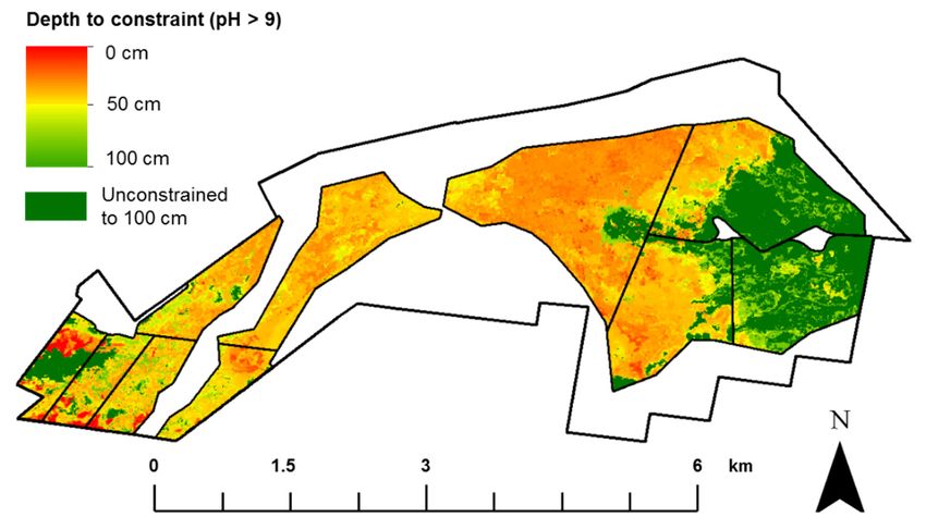
Agronomy 2019, 9, 251                                                                                 2 of 15

       While subsoil acidity is a widespread problem in other parts of Australia [8], subsoil alkalinity is
a more localized issue, and has consequently received less consideration in the literature. Many of the
soils in the cotton-growing valleys of eastern Australia are intrinsically alkaline due to the presence
of calcium and sodium carbonates, and this generally increases with depth [9]. Soils with a high pH
can limit the plant availability of certain nutrients, as well as cause toxicities [10]. At toxic levels,
root growth is inhibited, decreasing the amount of water and nutrients that can be accessed, producing
a detrimental impact on crop production [1]. The optimum pH (H2 O) range for most crops is generally
from 5.5 to 7, but this differs for individual crop types [11]. In soil with a pH (H2 O) of nine or greater,
it is likely that most crops would experience boron toxicity [12], as well as a considerable reduction
in the availability of important macro and micronutrients, including phosphorus, nitrogen, calcium,
magnesium, iron, copper, and zinc [13]. A pH (H2 O) greater than nine also suggests the presence of
sodium carbonates and high levels of soil sodicity, which indicates poor structural condition [12].
       Soil pH, and the depth at which a soil pH constraint is reached, can significantly vary across
fields [14], and this can result in spatially variable crop yields [15]. Digital soil mapping (DSM) has been
used extensively for evaluating the spatial distribution of soil pH at a range of spatial extents, from the
field [13], to the world [16]. Some studies solely produce pH maps for the topsoil (e.g., Kirk et al. [17]),
which lacks important information about subsoil pH. Other studies create maps of several depth
increments (e.g., Filippi et al. [18]), but this is often too much information from which to easily make
management decisions. The typical broadacre farmer in Australia now has access to a plethora of
data and information that relate to their farms [19], which is a great opportunity, but also a challenge
to gain useful insights. For a farmer that is experiencing a subsoil pH constraint in parts of their
farm, a single map of the depth at which that pH constraint begins would be invaluable. This would
assist in identifying areas where crop rooting depth may be inhibited, and help farmers implement
management practices to either rectify the issue or alter inputs according to the constrained production
potential. It is important to know the depth at which a pH constraint is reached within a fine vertical
resolution (e.g., 1 to 10 cm). However, most soil maps are produced at coarse resolutions, particularly
deeper in the soil profile. For example, the Globalsoilmap specifications are at 0–5, 5–15, 15–30, 30–60,
60–100, and 100–200 cm [16], and this creates difficulty in identifying exactly at what depth pH is a
limiting factor.
       There has been limited focus in the literature on mapping the depth of soil constraints. The study
reported here uses a novel modelling approach to predict and map the depth-to-soil pH constraint
(high alkalinity: pH >9 (H2 O)) on a dryland cotton and grain farm in the Namoi Valley in northern
New South Wales (NSW), Australia. A collection of spatial and temporal datasets were used for
modelling and mapping the depth-to-soil pH constraint, and the relationship with grain and cotton
yield mapping data was assessed.

2. Methods

2.1. Study Site
      This study was conducted on a mixed farming property—L’lara (30◦ 150 18” S, 149◦ 510 39” E), which
is located near Narrabri in the Namoi Valley in northern NSW, Australia. Summers in Narrabri are
very hot, while winters are cool. The long-term average precipitation for the study area is 658.5 mm,
and is summer-dominant [20]. The farm consists of 780 hectares of uncropped dryland grazing on
primarily native perennial pastures, and 1070 hectares of summer and winter dryland broadacre
cropping (Figure 1). The cropped area was the focus of this study, where cotton (Gossypium hirsutum L.),
and winter wheat (Triticum aestivum L.) are the dominant crops grown, with additional rotations of
canola (Brassica napus L.), and chickpea (Cicer arietinum L.). The soils of the cropping fields at L’lara
are classed as grey or brown Vertosols according to the Australia Soil Classification [21]. These soils
are primarily derived from alluvial deposits of basaltic sediments from the western side of the
Nandewar range.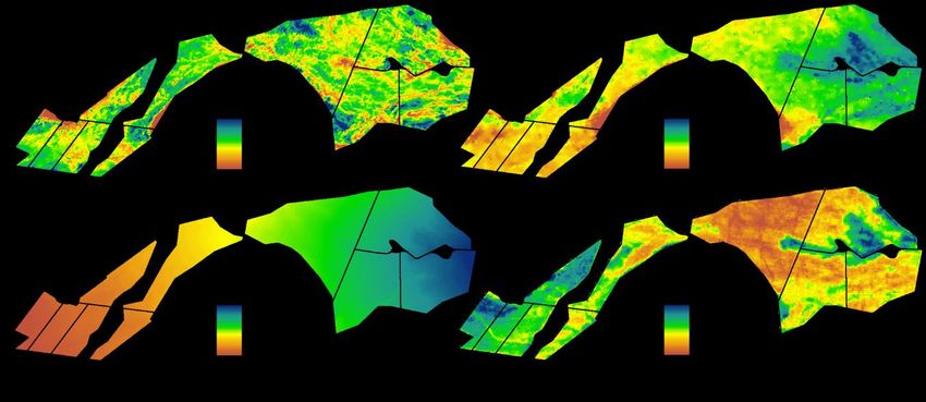
Agronomy 2019, 9, 251                                                                                       3 of 15
Agronomy 2019, 9, x FOR PEER REVIEW                                                                         3 of 15

     Figure 1.1. The
     Figure       Thearrangement
                      arrangementofof
                                    thethe cropping
                                         cropping     fields
                                                  fields      at L’lara,
                                                          at L’lara,     andlocation
                                                                     and the the location
                                                                                     withinwithin northern
                                                                                            northern       New
                                                                                                     New South
     South (NSW),
     Wales  Wales (NSW),    Australia.
                     Australia.

2.2.
2.2. Legacy
     Legacy Soil
            Soil Data
                 Data
     Soil data from
     Soil data  from 8080locations
                           locationssampled
                                      sampled  across
                                             across thethe  cropping
                                                         cropping      fields
                                                                   fields      in July
                                                                           in July 20172017
                                                                                        werewere  available.
                                                                                             available. Two
Two  subsamples    were   extracted  from the 0–0.1-  and  0.4–0.5-m  depth   increments  of each sampling
subsamples were extracted from the 0–0.1- and 0.4–0.5-m depth increments of each sampling location,
location,
resulting resulting
           in a totalin
                      ofa160
                           total of 160 subsamples.
                              subsamples.              All soil subsamples
                                            All soil subsamples                were air
                                                                   were air dried,   anddried,
                                                                                         groundandto ground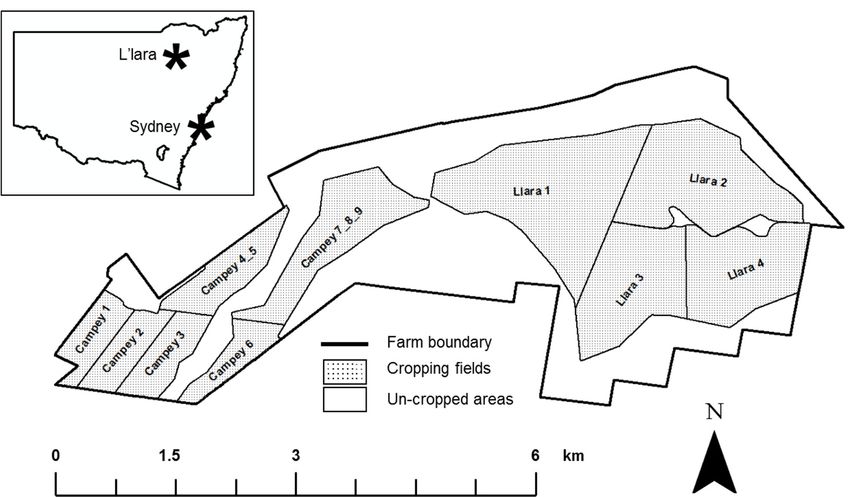
Agronomy 2019, 9, 251                                                                                                   4 of 15

Agronomy 2019, 9, x FOR PEER REVIEW                                                                                    4 of 15
2.3.2. Clustering Analysis and Site Selection
2.3.2. Clustering Analysis and Site Selection
      To create clusters of the study area with the data sources described above, k-means clustering
      To create
for strata        clusters of
            identification    theimplemented
                            was   study area with    thethe
                                                 using    data sources program
                                                            statistical  describedJMPabove,  k-means
                                                                                         ® Pro  11 (SASclustering
                                                                                                          Institute,
for strata  identification  was  implemented    using   the statistical program    JMP®    Pro 11
Cary, NC, USA). The optimum number of clusters for the study area was found to be eight (Figure 2),(SAS   Institute,
Cary,this
and    NC,wasUSA).   The optimum
                 determined          number
                               via the  elbow of  clusters
                                               method      for the
                                                         [27]. Thestudy
                                                                     elbowarea   was found
                                                                              method  looks atto the
                                                                                                 be eight   (Figure
                                                                                                      relationship
2), and this   was  determined   via  the elbow  method    [27]. The  elbow   method   looks  at
between the number of clusters and the proportion of variance explained and helps to identify thethe  relationship
between
point      the adding
       where    numberanother
                         of clusters  and would
                                  cluster  the proportion
                                                   provide of   variance
                                                             marginal      explained
                                                                        gain.         andofhelps
                                                                                The area     each to   identify
                                                                                                    cluster     the
                                                                                                             varied
point  where    adding   another  cluster  would   provide   marginal   gain.   The area  of each   cluster
from 39 to 228 ha. The 30 soil sampling locations were selected randomly within each cluster, with the       varied
from 39 of
number    to sites
              228 ha.
                   perThe  30 soil
                       cluster      sampling to
                                proportional  locations
                                                 the areawere    selected
                                                           of each  clusterrandomly   within each cluster, with
                                                                             (Figure 2).
the number of sites per cluster proportional to the area of each cluster (Figure 2).

      Figure 2. The distribution of the eight clusters derived from a k-means clustering analysis, and the
      Figure 2. The distribution of the eight clusters derived from a k-means clustering analysis, and the
      locations of the soil sampling sites across the study area.
      locations of the soil sampling sites across the study area.
2.3.3. Sampling Details
2.3.3. Sampling Details
      Soil cores at the 30 sites were extracted to a 1.0-m depth in July 2018. The cores were then
      Soil cores
subdivided    into at
                    fivethe   30 sites
                          depth          were(0–0.1,
                                  intervals     extracted    to 0.3–0.6,
                                                      0.1–0.3,  a 1.0-m0.6–0.8,
                                                                           depth and in July   2018.
                                                                                          0.8–1.0  m),The   cores in
                                                                                                       resulting    were   then
                                                                                                                      a total of
subdivided    into   five  depth   intervals   (0–0.1,  0.1–0.3,  0.3–0.6,  0.6–0.8,   and  0.8–1.0
150 subsamples. Equally to the legacy data, the subsamples were then air dried, and ground to
Agronomy 2019, 9, 251 5 of 15
Agronomy 2019, 9, x FOR PEER REVIEW 5 of 15
an RSX-1 gamma
instrument (Dualemradiometric
Inc., Milton,detector with aGamma
ON, Canada). 4 L sodium iodine data
radiometric crystal
were(Radiation Solutions
recorded using Inc.,
an RSX-1
Mississauga,
gamma ON, Canada).
radiometric detectorThe proximal
with soil sensing
a 4 L sodium iodinesurvey
crystalwas conducted
(Radiation on 24-m
Solutions swaths,
Inc., and the
Mississauga,
position
ON, was recorded
Canada). with differential
The proximal soil sensingGPS (DGPS)
survey equipment.onContinuous
was conducted 24-m swaths, surface layers
and the were
position
obtained
was by kriging
recorded with localGPS
with differential variograms [31] onto a Continuous
(DGPS) equipment. standard 5-m grid through
surface layers werethe obtained
software
VESPER
by [32].
kriging A 5-m
with localresolution
variogramsDEM was
[31] also
onto obtained from
a standard Spatial
5-m grid Services,
through theNSW Government
software VESPER [33].
[32].
The 90th percentile red band image from Landsat 7 described in the previous
A 5-m resolution DEM was also obtained from Spatial Services, NSW Government [33]. The 90thsection was also used
in this analysis.
percentile All spatial
red band imagedata
fromwere then extracted
Landsat ontoina the
7 described single 5-m resolution
previous grid also
section was usingused
the nearest
in this
neighbor method.
analysis. All spatial data were then extracted onto a single 5-m resolution grid using the nearest
neighbor method.
Table 1. Description of the data sources used in the mapping analysis.
Table 1. Description of the data sources used in the mapping analysis.
Data type Data description Resolution
ECa Data Type Dual EM-21S (0–3.0 m)
Data Description 5Resolution
m
On-farm
ECa
Gamma radiometrics Potassium (K) (0–3.0 m)
Dual EM-21S 5m 5m
On-farm
Gamma radiometrics Potassium (K) 5m
Elevation DEM 5m
Public Elevation DEM 5m
Public Landsat 7—red
Landsat 7—redband
band 90th
90thpercentile
percentile (2000–2017)
(2000–2017) 30 m30 m
( (
( (
Figure 3. The data sources used for digital soil mapping. (a) Soil
Soil ECa (0–3.0 m) from a Dual EM-21S,
(b) Gamma
(b) Gamma radiometrics
radiometricsK,
K,(c)
(c)DEM,
DEM,and
and(d)
(d)the
the90th
90thpercentile
percentile(2000–2017)
(2000–2017) red
red band
band from
from Landsat
Landsat 7.
7.
2.5.2. Modelling/Mapping Procedure
2.5.2.At
Modelling/Mapping
each of the 110 soilProcedure
sampling locations, the corresponding on-farm and publicly available
data At
described in Table 1 were collated.locations,
each of the 110 soil sampling A model the
to predict the relationship
corresponding on-farmbetween soil pHavailable
and publicly at 1-cm
increments
data describedandinthese
Tablecovariates was then
1 were collated. created
A model to using
predicta the
random forest model
relationship between [34].
soilThe
pH ‘ranger’
at 1-cm
package in the software R was used to create the model, which is essentially a
increments and these covariates was then created using a random forest model [34]. The ‘ranger’ fast implementation of
random
package forests for highRdimensional
in the software was used to data [35].
create the Instead of oneismodel
model, which for each
essentially depth
a fast increment, all
implementation of
were modelled together. This was possible, as each depth (at a 1-cm increment)
random forests for high dimensional data [35]. Instead of one model for each depth increment, all was stacked in the
data
wereframe, and together.
modelled depth was then
This included
was as aaspredictor
possible, each depth variable. Moreincrement)
(at a 1-cm specifically,was thestacked
central depth
in the
between the upper and lower depths was used (e.g., 0.5 cm for the 0–1-cm depth interval,
data frame, and depth was then included as a predictor variable. More specifically, the central depth and 99.5 for
the 99–100-cm depth interval). This model was then used to predict onto the
between the upper and lower depths was used (e.g., 0.5 cm for the 0–1-cm depth interval, and 99.5 5-m grid of the study
area using
for the the spatially
99–100-cm depthdistributed covariate
interval). This modeldataset.
was then This was
used to done
predictat onto
each the
1-cm 5-mincrement down
grid of the studyto
100
areacm, resulting
using in 100distributed
the spatially maps. Thecovariate
depth in dataset.
which the pHwas
This first reached
done a value
at each 1-cm of 9 or greater
increment down wasto
then identified for each 5-m grid point. A pH
100 cm, resulting in 100 maps. The depth in which the of 9 (H O) was selected, as this is an indicator
2 pH first reached a value of 9 or greater was of when
significant constraints
then identified for eachto5-m
growth
grid for most
point. A crops
pH ofis9 reached
(H2O) was as selected,
describedaspreviously. This information
this is an indicator of when
was then mapped across the study area, showing the depth-to-high soil pH constraint.
significant constraints to growth for most crops is reached as described previously. This information
was then mapped across the study area, showing the depth-to-high soil pH constraint.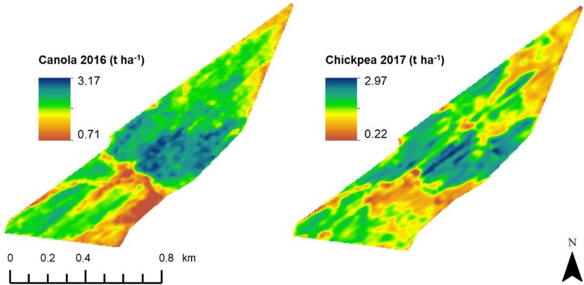
Agronomy 2019, 9, 251 6 of 15
Agronomy 2019, 9, x FOR PEER REVIEW 6 of 15
2.5.3. Model Quality and Validation
2.5.3. Model Quality and Validation
The quality of the model was tested by using leave-one-site-out cross-validation (LOSOCV).
The quality
This entailed of the model
iteratively was tested
removing all soilbydata
using leave-one-site-out
from each site, which cross-validation
ensured that data (LOSOCV). This
from different
entailed iteratively removing all soil data from each site, which ensured that data
depth increments of the same soil core were not included in both the calibration and validation datasets. from different
depth
This increments
LOSOCV of the same
was performed soil110
at all core were
sites, not109
with included in both
sites used the calibration
to predict and site
the remaining validation
each time.
datasets. This LOSOCV was performed at all 110 sites, with 109 sites used to predict
The results of the validation at every site were then combined, and the Lin’s concordance correlation the remaining
site each (LCCC)
coefficient time. The[36]results
and theofRMSE
the validation at every site
(root-mean-square were
error) werethen
usedcombined, andquality
to assess the the Lin’sof the
concordance correlation coefficient (LCCC) [36] and the RMSE (root-mean-square error) were used
model predictions. This cross-validation procedure was performed in two ways: (1) at 1-cm vertical
to assess the quality of the model predictions. This cross-validation procedure was performed in two
resolution (the splined observed pH data vs. the independently predicted pH data) and (2) at the
ways: 1) at 1-cm vertical resolution (the splined observed pH data vs. the independently predicted
original sampling depths of the observed data (observed pH data vs. predicted pH data at a 1-cm
pH data) and 2) at the original sampling depths of the observed data (observed pH data vs. predicted
resolution aggregated to the original sampling depths). The rationale for this was that the splining
pH data at a 1-cm resolution aggregated to the original sampling depths). The rationale for this was
procedure introduces some amount of uncertainty to the data [37] and validating by the second
that the splining procedure introduces some amount of uncertainty to the data [37] and validating by
approach avoids
the second approach this limitation
avoids thisaslimitation
the predictedas thedata are compared
predicted to the original,
data are compared to the un-splined
original, un-soil
pH data. To test the importance of different predictor variables in the model,
splined soil pH data. To test the importance of different predictor variables in the model, the the mean decrease
mean in
accuracy
decreasewas used, which
in accuracy wasisused,
basedwhich
on theismean
basedsquare
on theerror
mean(MSE).
square This shows
error theThis
(MSE). amount
showsby which
the
the random forest model prediction accuracy would decrease if that particular
amount by which the random forest model prediction accuracy would decrease if that particular variable is excluded.
The larger is
variable theexcluded.
mean decrease in accuracy
The larger the mean fordecrease
a predictor variable,for
in accuracy thea more important
predictor thatthe
variable, variable
more is
deemed.
importantAllthat
datavariable
analysisiswas performed
deemed. All data in analysis
the open-source software
was performed in R [38].
the open-source software R
[38].
2.6. Crop Yield Data and the Relationship with Depth-to-Soil pH Constraint
2.6. Crop Yield Data and the Relationship with Depth-to-Soil pH Constraint
2.6.1. Crop Yield Data
2.6.1. Crop
Yield dataYield
fromData
an on-harvester monitoring system was used to analyze the relationship with the
depth-to-soil pH constraint.
Yield data This yield monitoring
from an on-harvester monitor data consisted
system was of a variety
used of broadacre
to analyze crops from
the relationship withtwo
fields—Campey
the depth-to-soil4/5pH(C4/5) which
constraint. is 61
This hamonitor
yield in size, data
and L’lara 2 (L2)
consisted of awhich
varietyisof183 ha. Forcrops
broadacre C4/5,from
canola
two
was fields—Campey
grown in 2016, and4/5 (C4/5) which
chickpea in 2017is(Figure
61 ha in4a).
size,
ForandL2,L’lara
wheat2was (L2)grown
which in is 2016,
183 ha.
andFora summer
C4/5,
canola
cotton wasingrown
crop in 2016,
2017/2018 and 4b).
(Figure chickpea
The rawin 2017
yield(Figure
monitor 4a).data
For L2,
were wheat was grown
processed in 2016, spurious
by removing and a
summer
and extreme cotton
valuescrop in 2017/2018
following (Figure
the method 4b). The
of Taylor et al.raw
[39].yield
VESPERmonitor data was
software werethen
processed
used to bykrige
removing spurious and extreme values following the method of Taylor et al. [39].
the yield data onto the same 5-m grid as the soil modelling/mapping covariate data. The final surfaces VESPER software
wascorrected
were then usedand to krige the yield data
standardized usingonto thetotal
field same 5-m grid
yields as the
(grain soil modelling/mapping
weight at silo, or sum of bales covariate
of cotton
data. The final surfaces were corrected and standardized using field total
harvested). A 30-m internal buffered zone was applied around the paddock boundaries to remove yields (grain weight at silo,the
or sum of bales
low-yielding edgeofeffects,
cotton harvested).
and a 20-mAbuffer
30-m wasinternal
alsobuffered
placed on zonethewas applied
contour around
banks the(Figure
in L2 paddock 4a,b).
boundaries to remove the low-yielding edge effects, and a 20-m buffer was also placed on the contour
The rationale for removing these yield values was because the cause of low yield in these areas would
banks in L2 (Figure 4a,b). The rationale for removing these yield values was because the cause of low
likely be related to other factors as well as potential high soil pH.
yield in these areas would likely be related to other factors as well as potential high soil pH.
(a)
Figure 4. Cont.
Agronomy 2019, 9, 251 7 of 15
Agronomy 2019, 9, x FOR PEER REVIEW 7 of 15
Agronomy 2019, 9, x FOR PEER REVIEW 7 of 15
(b)
Figure
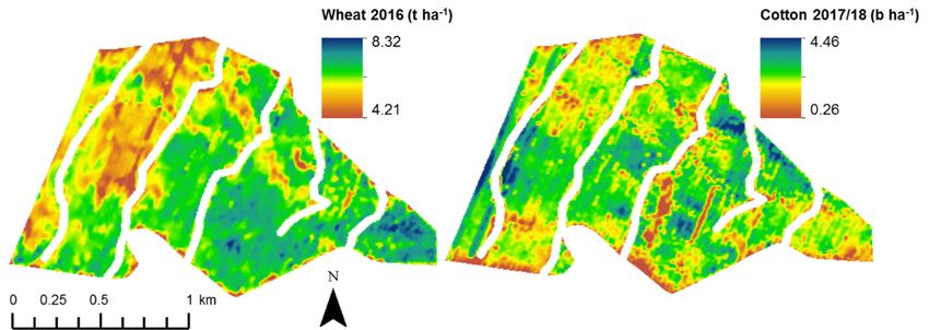
Figure 4. (a),
4. (a), Canola
Canola yield
yield forfor
thethe
20162016 season
season (left),
(left), andand chickpea
chickpea yield
yield for for
the the
20172017 season
season (right)
(right) from
frommonitor
a yield a yield monitor
for fieldfor field Campey
Campey 4/5 (C4/5).
4/5 (C4/5). (b), Wheat
(b), Wheat yield yield for2016
for the the 2016
seasonseason (left),
(left), andand cotton
cotton yield
foryield for the 2017/18
the 2017/18 season from
season (right) (right)a from
yieldamonitor
yield monitor forL’lara
for field field L’lara
2 (L2).2 (L2).
(b)
2.6.2. Relationship
2.6.2. Figure of
Relationship Crop
4. of
(a),Crop Yield
Canola yieldData
Yield thewith
Data
for Depth-to-Soil
withseason
2016 Depth-to-Soil pH Constraint
pH Constraint
(left), and chickpea Data
yield for theData
2017 season (right)
from a yield monitor for field Campey 4/5 (C4/5). (b), Wheat yield for the 2016 season (left), and cotton
The predicted
The yield fordepth-to-high
predicted depth-to-high
the soil pH
pHaconstraint
soilfrom
2017/18 season (right) yield monitordata
constraint data and
and
for field the
the
L’lara yielddata
yield
2 (L2). datawere
weremapped
mappedonon thethe
same 5-m grid, allowing the relationship to be easily analyzed. Boxplots
same 5-m grid, allowing the relationship to be easily analyzed. Boxplots were used to assess this, were used to assess
2.6.2. Relationship of Crop Yield Data with Depth-to-Soil pH Constraint Data
this, where
where data
data weregrouped
were groupedinin10-cm 10-cmintervals
intervals(depth-to-soil
(depth-to-soil pH pHconstraint),
constraint), showing
showing how
how thethe
distribution
distribution The
of predicted
ofyield
yield datadepth-to-high
data changed as
changed assoil
the pH
the constraint data
depth-to-soil
depth-to-soil pHand
pH the yield changed
constraint
constraint data changed
were for
mapped foron
each the paddock
paddock
each and
same 5-m grid, allowing the relationshipcorrelation
andcrop/season.
crop/season. TheTheSpearman
Spearman rank-ordertocorrelation
rank-order be easily analyzed.
coefficient,Boxplots
coefficient, werealso
rs, rwas used used
s , was
to assess
also usedto this,
toassess this
assess this
where data were grouped in 10-cm intervals (depth-to-soil pH constraint), showing how the
relationship.
relationship. Spearman’s
Spearman’s correlation
correlation is
is aa nonparametric
nonparametric measure
measure ofofthe
the direction
direction and strength
and strength of a a
of
distribution of yield data changed as the depth-to-soil pH constraint changed for each paddock and
relationship
relationship that
that
crop/season. exists
exists betweentwo
Thebetween
Spearman two variables
variables
rank-order based on
based
correlation on their ordered
their
coefficient, rs, was ranks.
ordered ranks. The
also usedThetomedian
median yield
assess this value
yield value
was calculated for
relationship. each 1-cm
Spearman’s depth interval,
correlation is a and the
nonparametricr
was calculated for each 1-cm depth interval, and the rs was then reported. s was then
measure ofreported.
the direction and strength of a
relationship that exists between two variables based on their ordered ranks. The median yield value
was calculated for each 1-cm depth interval, and the rs was then reported.
3. Results
3. Results
3. Results
3.1.3.1.
pHpH Variability
Variability inin
thetheStudy
StudyArea
Area
3.1. pHvalues
Soil Variability in the considerably
Study Area
Soil pHpH values variedvaried across the
considerably across the study
study area
area inin the
thetop
top100
100cm,
cm,withwitha alow
low ofof
6.16.1
at at
0–10
0–10 cm,cm,
andandaSoil
highapHhigh
of of varied
values
10.2 10.2
at at 30–60
considerably
30–60 cmacross
cm (Figure (Figure
5).the 5).
Asstudy As
depthareadepth increased,
in the top
increased, 100 median
cm, with
median pH soil
soila low of 6.1pH
values values
at increased,
0–10and
increased, cm,theandvariability
a high of 10.2 at 30–60 cm (Figure 5). As Soil
depth increased, median alkaline,
soil pH values
and the variability of observations decreased. Soil pH was generally alkaline, with a mean soilmean
of observations decreased. pH was generally
increased, and the variability of observations decreased. Soil pH was generally alkaline, with a mean
with a pH of
soil pH of 8.2
8.2 in the shallowestin the shallowest
layer (0–10 layerrising
cm), (0–10to
cm),
a risingpH
mean to of
a mean
9.3 inpH
theofdeepest
9.3 in the
layerdeepest
(80–100layer (80–
cm).
soil pH of 8.2 in the shallowest layer (0–10 cm), rising to a mean pH of 9.3 in the deepest layer (80–
100 cm).100 cm).
Figure 5. Boxplots of the distribution of soil pH (1:5 H2 O) with depth for 110 soil cores taken from
cropping fields at L’lara. Solid black lines inside boxes represent median values, and the dashed,
vertical grey line indicates the pH (H2 O) threshold of nine, deemed to have potential constraining
effects on crop growth.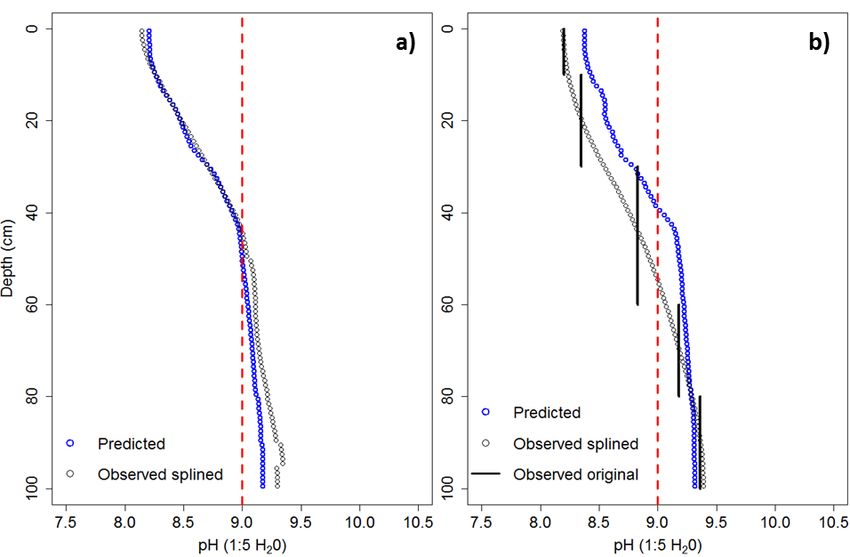
Agronomy 2019, 9, x FOR PEER REVIEW                                                                             8 of 15

      Figure 5. Boxplots of the distribution of soil pH (1:5 H2O) with depth for 110 soil cores taken from
      cropping fields at L’lara. Solid black lines inside boxes represent median values, and the dashed,
 Agronomy       9, 251line indicates the pH (H2O) threshold of nine, deemed to have potential constraining8 of 15
          2019, grey
      vertical
      effects on crop growth.

 3.2. Depth-to-Soil pH Constraint
 3.2. Depth-to-Soil pH Constraint
      The depth-to-high soil pH constraint map showed considerable spatial variability across the study
      The depth-to-high soil pH constraint map showed considerable spatial variability across the
 area (Figure 6). In total, 77% of the cropping fields had a strongly alkaline pH of nine somewhere
 study area (Figure 6). In total, 77% of the cropping fields had a strongly alkaline pH of nine
 within the top 100 cm (Table 2). The eastern section of the study area was largely unconstrained, with
 somewhere within the top 100 cm (Table 2). The eastern section of the study area was largely
 much of the middle section becoming constrained at 31–40 cm. The south-western section of L’lara had
 unconstrained, with much of the middle section becoming constrained at 31–40 cm. The south-
 high spatial variability in constraint conditions, with areas that were constrained in the top 1–10 cm,
 western section of L’lara had high spatial variability in constraint conditions, with areas that were
 and unconstrained within 100 cm, all within a short distance.
 constrained in the top 1–10 cm, and unconstrained within 100 cm, all within a short distance.

       Figure 6. Digital
       Figure 6. Digitalsoil
                         soilmap
                              mapofofthe depth
                                       the     in in
                                           depth  which soilsoil
                                                     which   pHpHconstraint (>9)(>9)
                                                                    constraint   is reached  across
                                                                                      is reached    the study
                                                                                                 across        area.
                                                                                                          the study
       area. Table 2. The area constrained at various depth intervals where pH >9 is first observed.

                                                                                                     Unconstrained
     Depth (cm)Table 2. The11–20
                  0–10       area constrained
                                   21–30      at various
                                           31–40   41–50 depth
                                                           51–60intervals
                                                                    61–70 where
                                                                           71–80pH 81–90
                                                                                    >9 is first observed.
                                                                                             91–100
                                                                                                     within 100 cm
      Area (ha)      11       16      183       339      128      51     23     32       37        4         Unconstrained
                                                                                                             245
Depth (cm)      0–10     11–20    21–30      31–40     41–50    51–60   61–70   71–80    81–90      91–100
       Area (%)      1.0      1.5     17.1      31.7     12.0     4.8    2.2    3.0      3.5      0.3        within 100 cm
                                                                                                             23.0
 Area (ha)       11       16       183        339       128      51       23      32        37         4          245
 Area (%)        1.0      1.5      17.1       31.7      12.0     4.8     2.2     3.0       3.5        0.3         23.0
 3.3. Model Quality and Variable Importance
 3.3. Model
      For theQuality
               randomand forest
                         Variable Importance
                                model,  the validated results showed an LCCC of 0.63, and an RMSE
 of 0.47 using LOSOCV when tested on the splined 1 cm data, and an LCCC of 0.66 and RMSE of
       For the random forest model, the validated results showed an LCCC of 0.63, and an RMSE of
 0.51 using LOSOCV when tested on the aggregated data at the original sampling depths (Table 3).
 0.47 using LOSOCV when tested on the splined 1 cm data, and an LCCC of 0.66 and RMSE of 0.51
 These statistics suggest that the model could spatially predict soil pH accurately (within ~0.5 pH units).
 using LOSOCV when tested on the aggregated data at the original sampling depths (Table 3). These
 Visual examples of the validation of soil pH predictions at 1-cm increments are shown in Figure 7,
 statistics suggest that the model could spatially predict soil pH accurately (within ~0.5 pH units).
 where Figure 7a shows the mean observed and predicted soil pH of all sampling sites, and Figure 7b
 Visual examples of the validation of soil pH predictions at 1-cm increments are shown in Figure 7,
 for a single randomly selected sampling site (Site 16). The soil pH predictions in these figures were
 where Figure 7a shows the mean observed and predicted soil pH of all sampling sites, and Figure 7b
 created using an independent calibration. This demonstrates that the random forest model can predict
 for a single randomly selected sampling site (Site 16). The soil pH predictions in these figures were
 the vertical distribution of soil pH.
 created using an independent calibration. This demonstrates that the random forest model can
 predict the vertical distribution of soil pH.
       Table 3. Validation prediction statistics for the soil pH model using leave-one-site-out cross-validation
       (LOSOCV) at a splined 1-cm resolution, and at the original sampling depth resolution.
       Table 3. Validation prediction statistics for the soil pH model using leave-one-site-out cross-
       validation (LOSOCV) at a splined    1-cm
                                       Lin’s      resolution,Correlation
                                              Concordance      and at the original sampling depth resolution.
         Validation Resolution                                                 Root Mean Square Error (RMSE)
                                              Coefficient (LCCC)
                                                            Lin’s Concordance            Root Mean
             SplinedValidation
                     1 cm       Resolution                0.63                                 0.47
                                                         Correlation Coefficient        Square Error
        Original sampling depth                           0.66                                   0.51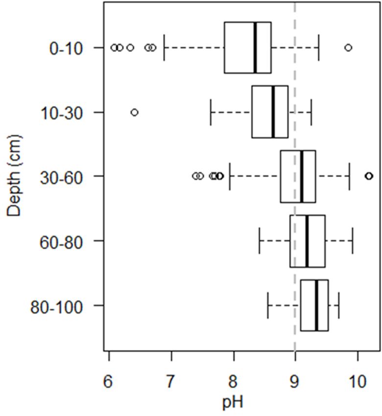
Agronomy 2019, 9, x FOR PEER REVIEW 9 of 15
Agronomy 2019, 9, x FOR PEER REVIEW 9 of 15
(LCCC) (RMSE)
Agronomy 2019, 9, 251
(LCCC) (RMSE) 9 of 15
Splined 1 cm 0.63 0.47
Splined 1 cm 0.63 0.47
Original sampling depth 0.66 0.51
Original sampling depth 0.66 0.51
( (
Figure
Figure 7. Observed soil
7. Observed soil pH
pH data
data splined
splined using
using equal-area
equal-area quadratic
quadratic smoothing
smoothing splines
splines (black
(black circles),
circles),
Figure 7. Observed soil pH data splined using equal-area quadratic smoothing splines (black circles),
and
and independently validated predicted data from the random forest model (blue circles) for the mean
independently validated predicted data from the random forest model (blue circles) for the mean
and
of independently validated predicted data from the random forest model (blue circles) for the mean
of all
all soil
soil sites
sites (a)
(a) and
and anan example
example soil
soil profile,
profile, Site
Site 16
16 (b).
(b). The
The observed
observed soil
soil pH
pH data
data atat the
the sampled
sampled
of all soil sites (a) and
depth an example soil profile, Site 16shown
(b). The observed soildashed
pH datalineatrepresents
the sampled
depth increments
increments (solid
(solid black
black lines)
lines) for
for Site
Site 16
16 is
is also
also shown in in (b). The red
(b). The red dashed line represents the
the
depth
pH increments
threshold of (solid
nine (H black
O). lines) for Site 16 is also shown in (b). The red dashed line represents the
pH threshold of nine (H2O). 2
pH threshold of nine (H2O).
The plot of the predictor variable importance showed that proximally sensed gamma radiometric
The plot of the predictor variable importance showed that proximally sensed gamma
K wasThe
theplot
most of the predictor
important predictorvariable importance
of soil pH showed
(Figure 8). This that proximally
was closely followed bysensed gamma
depth, and then
radiometric K was the most important predictor of soil pH (Figure 8). This was closely followed by
radiometric K was the most important predictor of soil pH (Figure 8). This was closely followed
other horizontally variable predictors, such as DEM, and soil ECa. Landsat 7 data of the 90th percentile by
depth, and then other horizontally variable predictors, such as DEM, and soil ECa. Landsat 7 data of
depth,
red and then
bandpercentile other horizontally
from the period 2000–2017 variable predictors, such as DEM, and soil ECa. Landsat 7 data of
the 90th red band from theproved
periodto2000–2017
be the least important
proved to be predictor of soil pH,predictor
the least important suggestingof
the 90th
that thispercentile
only red band
represents a fromcomponent
small the period of
2000–2017
soil proved
spatial to be the least important predictor of
variation.
soil pH, suggesting that this only represents a small component of soil spatial variation.
soil pH, suggesting that this only represents a small component of soil spatial variation.
Figure 8.
Figure 8. Mean decrease
Meandecrease in
decreasein accuracy
inaccuracy showing
accuracyshowing the
showingthe predictor
thepredictor variable
predictorvariable importance
variableimportance in predicting
importancein
in soil pH.
predictingsoil
soil pH.
Figure 8. Mean predicting pH.
3.4. The Relationship
3.4. The Relationship with
with Crop
Crop Yield
Yield and
and the
the Depth-to-Soil
Depth-to-Soil pH
pH Constraint
Constraint
3.4. The Relationship with Crop Yield and the Depth-to-Soil pH Constraint
Two fields,
fields, C4/5
C4/5 and
and L2,
L2, were
were used
used toto assess
assess the
the relationship
relationship between
between yield monitor data and
Two fields, C4/5 and L2, were used to assess the relationship between yield monitor data and
the predicted depth-to-soil pH constraint data. These These fields were selected due to the availability of
the predicted depth-to-soil pH constraint data. These fields were selected due to the availability of
yield data,
data, and
and the
the variation
variationininthe
thedepth
depthininwhich
whicha apH
pHofof9 was
9 waspredicted
predictedacross thethe
across field (Figure
field 6).
(Figure
yield data, and the variation in the depth in which a pH of 9 was predicted across the field (Figure
Boxplots were
6). Boxplots usedused
were to describe this this
to describe relationship, with with
relationship, the grouping of yield
the grouping data at
of yield 10-cm
data depth-to-soil
at 10-cm depth-
6). Boxplots were used to describe this relationship, with the grouping of yield data at 10-cm depth-
pH constraint intervals (Figure 9a,b). The 1–10 and 11–20 cm (to constraint) data are not used due to
the very few locations reaching a pH greater than 9 in the upper 20 cm. It was clear that as a soil pH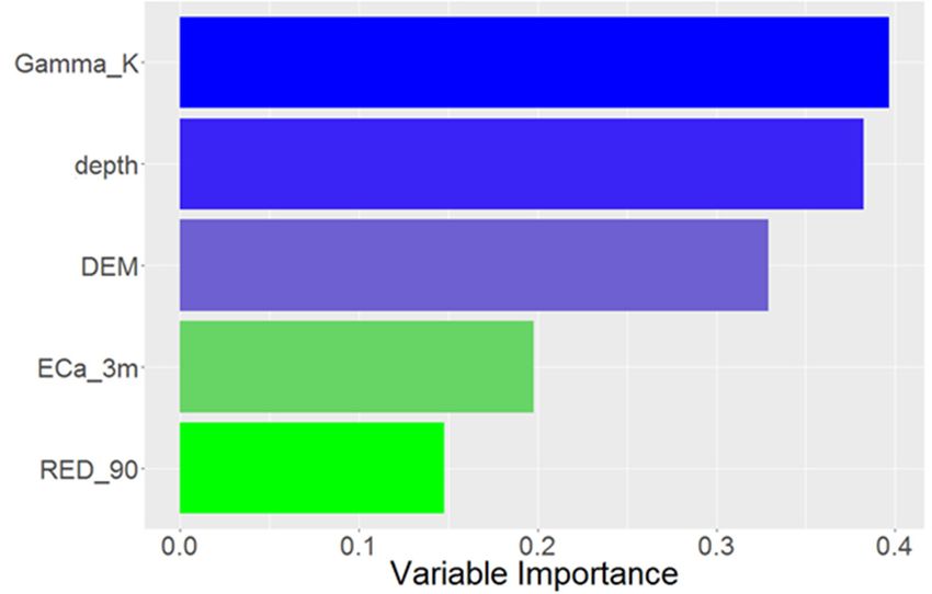
Agronomy 2019, 9, 251 10 of 15
Agronomy 2019, 9, x FOR PEER REVIEW 10 of 15
to-soil pH constraint intervals (Figure 9a,b). The 1–10 and 11–20 cm (to constraint) data are not used
constraint (>9) was deeper in the soil profile, the yield of most crops increased (Figure 9a,b). For all
due to the very few locations reaching a pH greater than 9 in the upper 20 cm. It was clear that as a
grain crops, the lowest median yield was observed where a soil pH constraint was reached in the
soil pH constraint (>9) was deeper in the soil profile, the yield of most crops increased (Figure 9a,b).
shallowest, well-observed layer (21–30 cm), and the highest median yield was observed where soil was
For all grain crops, the lowest median yield was observed where a soil pH constraint was reached in
deemed unconstrained
the shallowest, by pH inlayer
well-observed the top 100cm),
(21–30 cm. and
A clear
the spatial
highest correlation
median yield canwas
alsoobserved
be seen where
between
thesoil
grain crop yield maps (Figure 4a,b) and the depth-to-soil pH constraint map (Figure
was deemed unconstrained by pH in the top 100 cm. A clear spatial correlation can also be seen 6). For cotton,
thebetween
lowest the
median
grain yield was maps
crop yield observed where
(Figure 4a,b)aand
soilthe
pHdepth-to-soil
constraint was reached in
pH constraint mapthe(Figure
shallowest
6).
layer (21–30 cm), and an increase in median yield was observed as the depth-to-soil
For cotton, the lowest median yield was observed where a soil pH constraint was reached pH constraint
in the
increased to 61–70
shallowest layer cm.
(21–30However,
cm), andthis
an plateaued
increase inand slightly
median yielddeclined after this
was observed asdepth. The Spearman’s
the depth-to-soil pH
correlation
constraintanalysis
increasedrevealed
to 61–70that
cm.the relationship
However, betweenand
this plateaued the slightly
predicted depth-to-soil
declined after thispH constraint
depth. The
data and yieldcorrelation
Spearman’s monitor data ranged
analysis from strong
revealed that thetorelationship
weak (Table 4). Thethe
between strongest
predicted relationship
depth-to-soilwas
pH constraint
found with wheat data = 0.75),
(rs and yieldfollowed
monitor bydatacanola
ranged = 0.66),
(rsfrom strong to weak
chickpea = 0.58),
(rs(Table 4). and
The then
strongest
cotton
= 0.37).
(rs relationship was found with wheat (rs = 0.75), followed by canola (rs = 0.66), chickpea (rs = 0.58), and
then cotton (rs = 0.37).
(a)
(b)
Figure
Figure 9. 9.(a)
(a)Boxplots
Boxplots of the
the relationship
relationshipofofcrop yield
crop data
yield with
data the predicted
with depth-to-high
the predicted soil pHsoil
depth-to-high
constraint data for field Campey 4/5. (b) Boxplots of the relationship of crop yield
pH constraint data for field Campey 4/5. (b) Boxplots of the relationship of crop yield data withdata with thethe
predicted depth-to-high soil pH constraint data for field L’lara
predicted depth-to-high soil pH constraint data for field L’lara 2. 2.
Table 4. The
Table Spearman’s
4. The Spearman’scorrelation
correlation(r(rs )s) of
of the
the relationship betweenthe
relationship between thedepth-to-soil
depth-to-soil pH
pH constraint
constraint
map
mapdata and
data the
and median
the medianyield
yieldvalue
valueforforeach each 1-cm
1-cm depth incrementto
depth increment to100
100cm.
cm.
Campey
Campey4/5
4/5 L’lara 2 2
L’lara
Canola ‘16
Canola ‘16 Chickpea ‘17
Chickpea ‘17 Wheat ‘16
Wheat ‘16 Cotton ‘17/18‘17/18
Cotton
rs 0.66 0.58 0.75 0.37
rs 0.66 0.58 0.75 0.37Agronomy 2019, 9, 251 11 of 15
4. Discussion
4.1. Soil Alkalinity and Depth-to-Soil pH Constraint
Soil pH was generally alkaline and increased with depth. This is typical of Vertosols in the
cotton-growing valleys, and other studies in similar areas concur [18,40]. The depth in which a soil
pH greater than nine was reached was shown to be highly spatially variable across the study area.
Over half of the total area reached a pH of 9 within the shallow subsoil (21–40 cm), and approximately
77% of the area possessed an alkalinity constraint somewhere in the top 100 cm of the soil profile.
Soil alkalinity is often an inherent feature of the soils in these landscapes. However, it is possible that
the distribution of soil pH is being impacted by cultivation practices, which could be bringing the
more alkaline subsoils closer to the surface. Alkalinity in these soils are generally due to the presence
of calcium carbonates, but the extremely high pH values (>9) also indicate that sodium carbonates
are present. The presence of sodium carbonates also suggests that these soils possess high levels of
soil sodicity [41]. While alkalinity can reduce nutrient accessibility, cause toxicities, and inhibit root
growth for crops, soil sodicity is also known to have adverse impacts on crop productivity through
waterlogging and soil structural decline.
4.2. Modelling/Mapping
4.2.1. Modelling/Mapping Approach and Validation
The random forest model could predict the spatial distribution of soil pH well, and the approach
proved successful in identifying the depth-to-soil pH constraint at a 1-cm vertical resolution to a 100-cm
depth. The LOSOCV on the splined 1-cm data showed an LCCC of 0.63, and an RMSE of 0.47, and an
LCCC of 0.66 and RMSE of 0.51 when tested on the data at the original sampling depths. The fact that
these two cross-validation techniques showed very similar validation statistics is optimistic. The second
cross-validation approach validates predictions with the original, un-splined data, which suggests
that the splining procedure is creating a relatively small amount of uncertainty in the data, giving
confidence in the developed mapping approach.
While this study was performed on a 1070-ha farm, there is promise for implementing this
approach over larger areas. However, the fine-resolution splining of soil property data results in a
much larger amount of data compared to typical DSM methods, and implementing this with very
large datasets could become computationally restrictive. One opportunity to reduce the computational
load of this approach is to fit the soil property at 5-cm increments with the splines as opposed to 1-cm
increments. This would still be at a fine enough vertical resolution to inform management decisions
for land managers but would significantly reduce the dataset size. An alternative would be to use the
approach of Orton et al. [37] who presented a geostatistical approach to predict in 3D at any vertical
resolution using observations from different vertical supports (e.g., soil horizons). This would remove
the need for using splines to create the finely spaced vertical dataset. Adopting the approach by Orton
et al. [37] also bypasses the uncertainty introduced by the splining process, although, as discussed,
the results in the current study suggested that this was relatively small (Table 3). The uncertainty in
imputed values is commonly ignored in DSM studies that use splined soil data.
Few studies have used DSM approaches to map the depth-to-soil constraints, but there has
been considerable research in mapping the depth to bedrock [42–44]. The methods used in these
studies are essentially traditional DSM approaches, and differ significantly from the current study.
For example, data for the depth to which bedrock is reached is commonly available from mining
exploration and bore hole drilling exercises, and Wilford et al. [44] used a database of these observations
to create depth-to-bedrock maps of Australia using a Cubist model. In contrast, rather than use direct
observations of the depth of the target variable/constraint, the current study uses splined soil pH data,
and machine learning to predict the depth in which an alkalinity constraint is reached at each 1-cm
vertical increment, which is then combined to create a depth-to-soil pH constraint map. It is typicallyAgronomy 2019, 9, 251 12 of 15
not easy to identify the depth at which a soil constraint occurs in the field, but this approach helps
overcome this. Another advantage of the approach used in this study is that it could be applicable to
any soil property, not just soil alkalinity.
4.2.2. Predictor Variables
Only four spatial predictor variables were used for modelling and mapping (Table 1), whereas
most other DSM studies use a much larger suite of predictor variables. The rationale for this was that the
variables used in the current study were of a fine spatial resolution (5–30 m), with the on-farm collected
data (ECa and gamma radiometrics) known to reflect soil spatial variability very well. The most
important covariate for the soil pH random forest model was proximally sensed gamma radiometrics
K (5 m). This covariate is often highly correlated with soil type and represents fine-scale soil spatial
variability due to intensive measurements collected in this study. The second most important covariate
for the soil pH random forest model was depth, which is logical, as pH in these soils increases as
depth increases. The model could predict the vertical distribution of soil pH well, and this is due to
the inclusion of depth as a predictor variable. This concept is demonstrated in Figure 7. The DEM
data (5 m) represented broader trends across the study area and possessed lower short-range spatial
variability (Figure 4), but this proved to be an important predictor variable. The ECa data (5 m) was
the second least important predictor, as the high spatial variability (Figure 4) did not seem to represent
the spatial variation of soil pH particularly well. The least important predictor was the 90th percentile
red band (30 m), which could be due to the coarser spatial resolution compared to the other predictor
variables, and that it did not sufficiently reflect the spatial distribution of soil pH.
4.3. Relationship between Depth-to-Soil pH Constraint and Crop Yield
The relationship between the depth-to-soil pH constraint map and cotton and grain yield was
explored for fields C4/5 and L2. It was clear that the deeper in the soil profile a pH constraint greater
than nine was reached, the yield of all crops generally increased. The relationship between yield and
the depth-to-soil pH constraint data was stronger for the grain crops than for cotton. The Spearman’s
correlation was highest for wheat (rs = 0.75), followed by canola (rs = 0.66), chickpea (rs = 0.58),
and then cotton (rs = 0.37). This suggests that cotton was relatively unaffected by an alkalinity constraint
compared to the grain crops. Cotton is almost solely grown in the alkaline Vertosols of the alluvial
valleys of eastern Australia and is therefore well-accustomed to these soils. This could be a possible
reason for the weaker relationship. However, crop yield is a function of climate, soil, and management,
and their interaction, and this could vary from season to season [45]. Future research should focus on
using a longer time-series of yield data to assess the variation in the relationship between yield and
the depth-to-soil pH constraint to account for this. The approach developed in this study should also
be applied to a larger spatial extent in the future, as this information could be useful in identifying
constraints to yield at a broader scale to guide policy decisions.
In field C4/5, similar spatial patterns were observed for canola in 2016 and chickpea in 2017.
In contrast, the wheat yield maps in 2016 and the cotton yield maps in 2017/2018 showed some differing
spatial patterns, with some of the highest yielding areas for cotton being the lowest yielding for
wheat. These inconsistently yielding or flip-flop patterns have been commonly observed in other
studies [45–47], and often point to a temporary constraint, rather than a permanent soil constraint
such as high soil pH levels. Despite the important role that soil pH plays on crop productivity,
few studies have looked at the impact of within-field soil pH variability on crop yield, let alone how
the depth-to-soil pH constraint relates to this. Shatar and McBratney [48] assessed the relationship
between soil pH (15–30 cm) and sorghum yield, and found that pH was a limiting factor in some areas
of the field. A study by Schepers et al. [49] also found that management zones (MZ) with varying pH
levels within a field displayed a marked difference in corn grain yield over several seasons. The MZ
with the lowest mean pH (6.41) showed the highest yield, and the MZ with the highest mean pHAgronomy 2019, 9, 251 13 of 15
(7.43) displayed the lowest yields. In contrast, Adeoye and Agboola [50] saw a significant positive
correlation between the soil pH and the relative yield of maize.
The results found in this study suggest that the depth-to-soil pH constraint can directly influence
crop yield. However, as aforementioned, these very high levels of soil pH are a strong indicator
that soil sodicity is also an issue. Soil sodicity is a common issue in the alluvial Vertosols of eastern
Australia [4,51,52] and is deemed to be one of the biggest constraints to crop production in these
regions [1]. High sodicity levels of soil have a greater capacity to inhibit root growth than high pH
levels. This results in a smaller volume of soil that is accessible to crops, and consequently a smaller
amount of water and nutrients available for crop development [53]. Further research should look at
soil sodicity and the impact it has on crop yield variability in the study area. Future work should also
use the approach presented to estimate the reduction in the soil water holding capacity and therefore
yield potential, caused by soil constraints.
5. Conclusions
High levels of soil alkalinity were observed in the study area, particularly at depth. The random
forest model to predict soil pH distribution showed high quality predictions when testing with
LOSOCV, with an LCCC of 0.63–0.66, and an RMSE of 0.47–0.51. The overall approach to identify the
depth at which a pH alkalinity constraint (>9) occurred at fine vertical resolution (1 cm) at a farm scale
proved successful and showed promise for identifying other important subsoil constraints. The study
revealed that the shallower in the soil profile a pH constraint was reached, the generally smaller the
crop yield. A strong relationship was found for wheat, canola, and chickpea, with a weaker relationship
for cotton. The output of a single map showing the depth at which a soil alkalinity constraint occurs is
a valuable, concise piece of information for farmers and land managers, and is a promising avenue to
guide the remediation of soil constraints, or the tailoring of crop management inputs to account for
these constraints.
Author Contributions: Conceptualization, P.F. and T.F.A.B.; Formal analysis, P.F., E.J.J. and B.J.G.; Investigation,
B.J.G.; Methodology, P.F., E.J.J., B.M.W. and T.F.A.B.; Project administration, P.F.; Resources, G.W.R.; Validation, P.F.
and T.F.A.B.; Writing—original draft, P.F. and B.J.G.; Writing—review and editing, P.F., E.J.J., B.M.W., G.W.R. and
T.F.A.B.
Funding: This research was partly funded by grants provided by the Cotton Research and Development
Corporation (DAN1801, US1802), the Grains Research and Development Corporation (US00087), and the
University of Sydney.
Acknowledgments: Thank you to the two anonymous reviewers for their helpful feedback, and to the Commercial
Cropping Supervisor of L’lara—Kieran Shephard, for his assistance in gathering the data.
Conflicts of Interest: The authors declare no conflict of interest.
References
1. Dang, Y.P.; Dalal, R.C.; Routley, R.; Schwenke, G.D.; Daniells, I. Subsoil constraints to grain production in the
cropping soils of the north-eastern region of Australia: An overview. Aust. J. Exp. Agric. 2006, 46, 19–35.
[CrossRef]
2. Odeh, I.O.A.; Todd, A.J.; Triantafilis, J.; McBratney, A.B. Status and trends of soil salinity at different scales:
The case for the irrigated cotton growing region of eastern Australia. Nutr. Cycl. Agroecosyst. 1998, 50,
99–107. [CrossRef]
3. Odeh, I.O.A.; Onus, A. Spatial analysis of soil salinity and soil structural stability in a semiarid region of
New South Wales, Australia. Environ. Manag. 2008, 42, 265–278. [CrossRef] [PubMed]
4. McKenzie, D.C.; Abbott, T.S.; Chan, K.Y.; Slavich, P.G.; Hall, D.J.M. The nature, distribution and management
of sodic soils in New-South-Wales. Soil Res. 1993, 31, 839–868. [CrossRef]
5. Dodd, K.; Guppy, C.; Lockwood, P.; Rochester, I. The effect of sodicity on cotton: Plant response to solutions
containing high sodium concentrations. Plant Soil 2010, 330, 239–249. [CrossRef]
6. McGarry, D. Soil compaction and cotton growth on a Vertisol. Soil Res. 1990, 28, 869–877. [CrossRef]Agronomy 2019, 9, 251 14 of 15
7. Antille, D.L.; Bennett, J.M.; Jensen, T.A. Soil compaction and controlled traffic considerations in Australian
cotton-farming systems. Crop Pasture Sci. 2016, 67, 1–28. [CrossRef]
8. De Caritat, P.; Cooper, M.; Wilford, J. The pH of Australian soils: Field results from a national survey. Soil Res.
2011, 49, 173–182. [CrossRef]
9. Knowles, T.A.; Singh, B. Carbon storage in cotton soils of northern New South Wales. Soil Res. 2003, 41,
889–903. [CrossRef]
10. Läuchli, A.; Grattan, S.R. Soil pH extremes. Plant Stress Physiol. 2012, 194–209.
11. Hazelton, P.; Murphy, M. Interpreting Soil Test Results: What Do All the Numbers Mean? CSIRO Publishing:
Victoria, Australia, 2007.
12. Slattery, W.J.; Conyers, M.K.; Aitken, R.L. Soil pH, aluminium, manganese and lime requirement. In Soil
Analysis: An Interpretation Manual; Peverill, K.I., Sparrow, L.A., Reuter, D.J., Eds.; CSIRO: Collingwood,
Australia, 1999; pp. 103–128.
13. McKenzie, N.; Jacquier, D.; Isbell, R.; Brown, K. Australian Soils and Landscapes: An Illustrated Compendium;
CSIRO Publishing: Clayton, Australia, 2004.
14. Adamchuk, V.I.; Lund, E.D.; Reed, T.M.; Ferguson, R.B. Evaluation of an on-the-go technology for soil pH
mapping. Precis. Agric. 2007, 8, 139–149. [CrossRef]
15. Taylor, J.C.; Wood, G.A.; Earl, R.; Godwin, R.J. Soil factors and their influence on within-field crop variability,
Part II: Spatial analysis and determination of management zones. Biosyst. Eng. 2003, 84, 441–453. [CrossRef]
16. Arrouays, D.; Grundy, M.G.; Hartemink, A.E.; Hempel, J.W.; Heuvelink, G.B.M.; Hong, S.Y.; Lagacherie, P.;
Lelyk, G.; McBratney, A.B.; McKenzie, N.J.; et al. Globalsoilmap: Toward a fine-resolution global grid of soil
properties. Adv. Agron. 2014, 125, 93–134.
17. Kirk, G.J.D.; Bellamy, P.H.; Lark, R.M. Changes in soil pH across England and Wales in response to decreased
acid deposition. Glob. Chang. Biol. 2010, 16, 3111–3119. [CrossRef]
18. Filippi, P.; Cattle, S.R.; Bishop, T.F.A.; Odeh, I.O.A.; Pringle, M.J. Digital soil monitoring of top- and sub-soil
pH with bivariate linear mixed models. Geoderma 2018, 322, 149–162. [CrossRef]
19. Bramley, R.G.V.; Ouzman, J. Farmer attitudes to the use of sensors and automation in fertilizer decision-making:
Nitrogen fertilization in the Australian grains sector. Precis. Agric. 2018. [CrossRef]
20. Bureau of Meteorology. Monthly climate statistics—Narrabri West Post Office (053030). Available online:
http://www.bom.gov.au/climate/averages/tables/cw_053030.shtml (accessed on 18 December 2018).
21. Isbell, R.F. The Australian Soil Classification; CSIRO Publishing: Melbourne, Australia, 1996.
22. Boydell, B.; McBratney, A.B. Identifying potential management zones from cotton yield estimates. Precis. Agric.
2002, 3, 9–23. [CrossRef]
23. Grundy, M.J.; Rossel, R.V.; Searle, R.D.; Wilson, P.L.; Chen, C.; Gregory, L.J. Soil and landscape grid of
Australia. Soil Res. 2015, 53, 835–844. [CrossRef]
24. Geoscience Australia. Geoscience Australia, 1 Second SRTM Digital Elevation Model (DEM). Bioregional
Assessment Source Dataset. Available online: http://data.bioregionalassessments.gov.au/dataset/9a9284b6-
eb45-4a13-97d0-91bf25f1187b (accessed on 4 December 2018).
25. Minty, B.R.S.; Franklin, R.; Milligan, P.R.; Richardson, L.M.; Wilford, J. The radiometric map of Australia.
Explor. Geophys. 2009, 40, 325–333. [CrossRef]
26. Gorelick, N.; Hancher, M.; Dixon, M.; Ilyushchenko, S.; Thau, D.; Moore, R. Google Earth Engine:
Planetary-scale geospatial analysis for everyone. Remote Sens. Environ. 2017, 202, 18–27. [CrossRef]
27. Kodinariya, T.M.; Makwana, P.R. Review on determining number of Cluster in K-Means Clustering. Int. J.
2013, 1, 90–95.
28. Bishop, T.F.A.; McBratney, A.B.; Laslett, G.M. Modelling soil attribute depth functions with equal-area
quadratic smoothing splines. Geoderma 1999, 91, 27–45. [CrossRef]
29. Malone, B.P.; McBratney, A.B.; Minasny, B.; Laslett, G.M. Mapping continuous depth functions of soil carbon
storage and available water capacity. Geoderma 2009, 154, 138–152. [CrossRef]
30. Malone, B. Ithir: Soil Data and Some Useful Associated Functions, R Package Version 1.0. 2015. Available
online: https://rdrr.io/rforge/ithir/ (accessed on 20 March 2019).
31. Haas, T.C. Kriging and automated variogram modelling within a moving window. Atmos. Environ. 1990, 24,
1759–1769. [CrossRef]You can also read