Scattering Cancellation Technique for Acoustic Spinning Objects
←
→
Page content transcription
If your browser does not render page correctly, please read the page content below
Scattering Cancellation Technique for Acoustic Spinning Objects

                                                                             M. Farhat,1, ∗ S. Guenneau,2 A. Alù,3 and Y. Wu1, †
                                                        1
                                                            Computer, Electrical, and Mathematical Science and Engineering (CEMSE) Division,
                                                                             King Abdullah University of Science and Technology
                                                                                (KAUST), Thuwal 23955-6900, Saudi Arabia
arXiv:2004.01482v1 [physics.class-ph] 3 Apr 2020

                                                                                   2
                                                                                       UMI 2004 Abraham de Moivre-CNRS,
                                                                     Imperial College London, London SW7 2AZ, United Kingdom.
                                                                        3
                                                                            Photonics Initiative, Advanced Science Research Center,
                                                                    City University of New York, New York, New York 10031, USA
                                                                                              (Dated: April 6, 2020)

                                                                                                   Abstract
                                                        The scattering cancellation technique (SCT) has proved to be an effective way to render static
                                                   objects invisible to electromagnetic and acoustic waves. However, rotating cylindrical or spherical
                                                   objects possess additional peculiar scattering features that cannot be cancelled by regular SCT-
                                                   based cloaks. Here, a generalized SCT theory to cloak spinning objects, and hide them from static
                                                   observers, based on rotating shells with different angular velocity is discussed. This concept is
                                                   analytically and numerically demonstrated in the case of cylinders, showing that generalized SCT
                                                   operates efficiently in making rotating objects appear static to an external observer. Our proposal
                                                   extends the realm of SCT, and brings it one step closer to its practical realization that involves
                                                   moving objects.

                                                   ∗
                                                       Electronic address: mohamed.farhat@kaust.edu.sa
                                                   †
                                                       Electronic address: ying.wu@kaust.edu.sa

                                                                                                         1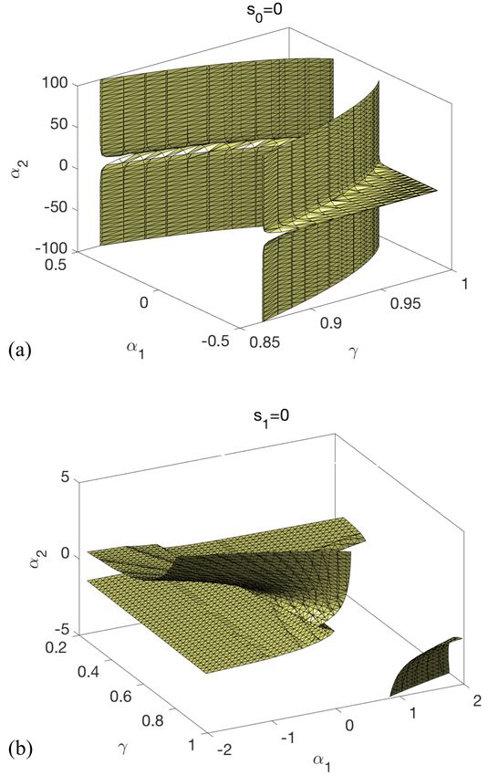
I.    INTRODUCTION

     Inspired by the concept of photonic crystals [1–4] and photonic crystal fibres [5–8], a new
class of acoustic materials has emerged during the 1990s. These so-called phononic crystals
(PCs), consist of a periodic arrangement of at least two materials with different densities
[9–12]. These materials were shown to possess a frequency range over which sound wave
propagation is prohibited (phononic bandgap) [9, 10]. These forbidden bands can also result
in singular properties of sound waves, e.g., negative refraction at the interface between
a classical medium and a phononic crystal [13–15], ultrasound tunneling [16], or tunable
filtering and demultiplexing [17], to cite a few [18–23]. These PCs are difficult to miniaturize,
as the bandgap appears at wavelengths in the same order as the period of the PCs, meaning
a low frequency bandgap requires a large PC [24, 25]. To overcome this major hurdle,
active research has been directed towards other concepts involving local resonances [26, 27],
that best operate when the periodicity is much smaller than the wavelength (this is the
so-called quasi-static, or long-wavelength limit). For instance, composite structures formed
by locally resonating meta-atoms, so-called metamaterials (MMs) made their appearance at
the turn of the century, both for electromagnetic [28–31] and acoustic [32] waves. Based on
analogies drawn from optical MMs, an acoustic MM consists of a heterostructure formed
of resonant inclusions having characteristic dimensions smaller than the wavelength of the
wave propagating in the medium, and vibrating on their natural modes of resonance [33].
     Controlling the propagation of waves using these engineered MMs is thus a considerable
opportunity [34, 35]. For example, one can protect buildings from seismic waves [36, 37] or
tsunamis [38–41] by means of a large scale metamaterial which may guide the acoustic/elastic
energy out of the area to be protected and may considerably attenuate the amplitude of the
impinging waves. Defense applications are potentially very important as well, with the
possibility, for example, of fabricating stealth systems (invisibility cloaks) [35]. The term
”invisibility cloak” designates a coating whose material parameters, determined by the opti-
cal transformation process, make it possible to deflect any electromagnetic or elastodynamic
wave [42–44]. If one places an object in the isolated interior area, then no incident wave
can interact with this object since the cloak detours wave trajectories around it in such a
way that for any external observer the field appears to be undisturbed. In other words, the
object is both undetectable (invisible) and protected. Note that the concept of invisibility

                                               2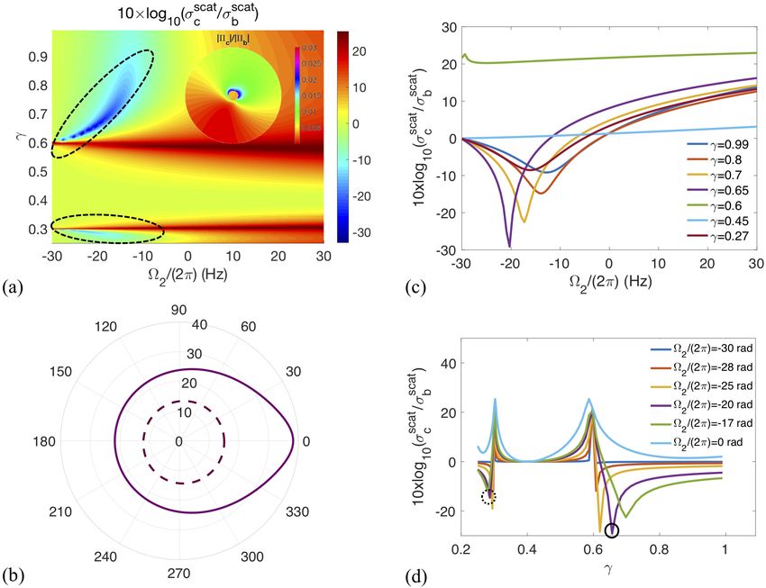
is distinct from that of stealth [45]. The primary purpose of a stealth coating is to cancel
the reflection coefficient in certain directions (typically those of a detection antenna). To
do this, the idea is to absorb the incident waves or to reflect them to another direction.
Interestingly, some species of moths have acquired dynamic acoustic camouflaging features
thanks to some microstructure reminiscent of metamaterial surfaces [46]. Conversely, in an
invisible device, one cancels both the reflection coefficient and the absorption, and one makes
the transmission coefficient ideally unitary. The object included in the coating then has a
zero electromagnetic/acoustic size and it has no ”shadow” [35]. Other cloaking strategies
were subsequently proposed through homogenization [47–49], and/or scattering cancellation
technique (SCT) [50, 51], and even suggested for other types of waves [52–54].
   All the above-mentioned devices and techniques operate for static objects, i.e., at rest.
For instance, moving or rotating objects possess intrinsically different scattering signature
[55–64] and require special treatment [65, 66]. Some intriguing applications were put for-
ward with spinning elements such as gyroscopes [67, 68] and waveguide rotation sensors
[66]. In order to realize efficient cloaking devices for such rotating devices, one first needs to
characterize the scattering response from these acoustic objects and then analyze the feasi-
bility and physical difference of cloaking mechanism. A recent study for example considered
cloaking structures that are moving in a rectilinear way, using spatiotemporal properties
to counter the Doppler effect [69, 70]. A theory of a space-time cloak was also proposed
to make a time interval undetectable for an observer [71] and further demonstrated exper-
imentally in a highly dispersive optical fibre [72]. However, cloaking rotating objects was
not achieved in any context. In the present paper, the use of the scattering cancellation
technique [51, 73–76] to render spinning objects invisible for acoustic waves is proposed.
   The rest of the paper is organized as follows. In the background and problem setup
section, the equations of motion of a spinning acoustic object and its dispersion relation,
that permit the study of acoustic scattering from multilayered spinning structures are put
forward. In the following section, using Bessel expansions of the pressure fields, it is shown
the possibility of cancelling the leading scattering orders from spinning objects by coating
them with shells of tailored spinning velocity. In this section the effect of geometrical
parameters and spinning velocity amplitude, on the scattering reduction is also analyzed.
Finally, the obtained results are summarized in the concluding remarks.

                                               3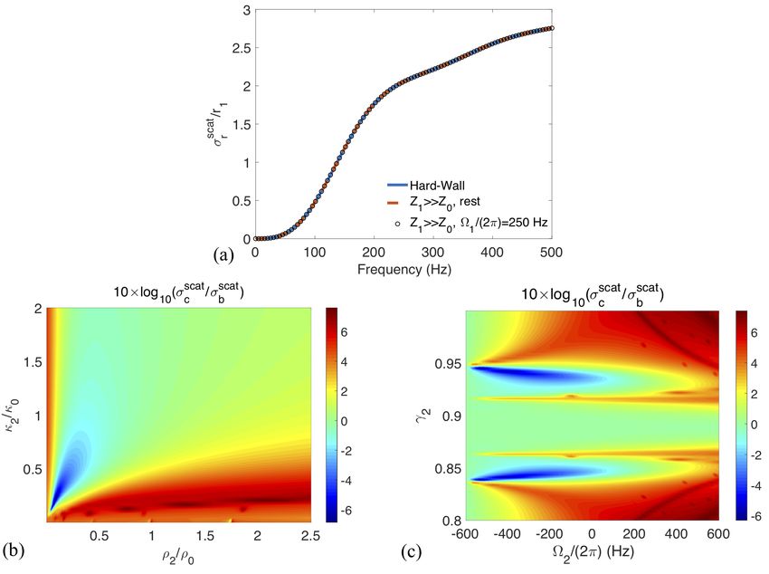
II. BACKGROUND AND PROBLEM SETUP
A. Acoustic equation in rotating media
Let us consider time-harmonic waves, with dependence upon time t proportional to e−iωt ,
where ω is the angular wave frequency. One also assumes structures with cylindrical symme-
try (invariance) [See Fig. 1(a),] i.e., proportional to einθ so that derivatives in the azimutal
direction θ produce terms of the form in, where n is an integer and i2 = −1. One starts
by invoking the mass and momentum conservation laws of acoustics and one expresses
them in the laboratory frame of reference [77]. This is done by using the Eulerian speci-
fication of the flow field, i.e. by replacing time derivatives with material derivatives, i.e.,
∂t0 (·) → ∂t (·) + u · ∇(·), where the 0 denotes derivatives taken in the rest frame of the moving
fluid. Also, u = u0 + v is the total velocity of the flow, whereas u0 is the bulk velocity, and
v is the acoustical perturbation velocity. This results in modified conservation equations
(See Appendix A).
One combines the modified equations, i.e., Eqs. (A3)-(A4) of the Appendix, by writing
down each component [for instance, Eq. (A3) contains two components, while Eq. (A4)
contains a single component.] Then, one uses u0 · ∇ = Ω1 ∂/∂θ and one linearizes the
equations, by keeping only first order quantities of acoustic perturbations, e.g., terms such
as (v · ∇)v are neglected, as shown in Appendix A [77]. One thus obtains a linear system
(of order 3) in terms of the variables p1 , vr,1 , and vθ,1 (assuming that the z-components of
the fields are zero, as it is assumed in this first example, infinitely extended cylinders in the
z-direction). This system of coupled partial differential equations (PDEs) can be expressed,
in cylindrical coordinates, using the differential operator D̃, as D̃ (vr,1 , vθ,1 , p1 )T = 0, with
(·)T denoting the transpose of the vector in parentheses, i.e.,
−1
ζ
n,1 −2Ω 1 ρ 1 ∂r
vr,1
2Ω1 ζn,1 (ρ1 r)−1 in vθ,1 = 0 . (1)
−1 −1 −1 −2
r + ∂r r in ρ1 c1 ζn,1 p1
In this coupled differential system, one denotes ∂r = ∂/∂r and the modified angular fre-
quency ζn,1 = i(nΩ1 − ω). From the system of Eq. (1), one derives the equation verified by
the pressure p1 , in the cylindrical coordinates, that is
∂ 2 p1 1 n2
2
+ p1 + βn,1 − 2 p1 = 0 , (2)
∂r2 r r
4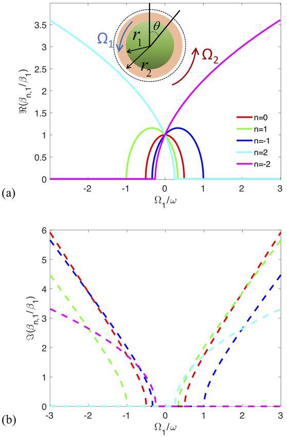
which is the Helmholtz equation expressed in cylindrical coordinates, assuming an effective
wavenumber                                 s
                                                         2
                                               − 4Ω21 + ζn,1
                                  βn,1 =                       .                           (3)
                                                    c21
One verifies that for Ω1 = 0, one recovers the classical dispersion β1 = ω/c1 , with c1 =
p
 κ1 /ρ1 the speed of sound inside the object (all parameters related to the object are denoted
with subscript 1 and those related to free-space with subscript 0). The behavior of βn,1 ,
i.e. the spinning effective wavenumber is depicted in Fig. 1(b). As the parameter ζn,1 is
complex, βn,1 possesses both imaginary and real parts (i.e. damping). For example, for
β0,1 (i.e. n = 0,) in the domain |α1 | = |Ω1 /ω| ≤ 1/2, only the real part exists and decays
exponentially, while reaching 0 for α1 = ±1/2. The imaginary part is zero in this domain
and increases quasi-linearly. The orders n = ±1 possess similar and symmetric behavior.
The orders n = ±2 have slightly different behavior, which is not symmetric with respect to
α1 . It should be mentioned that for α1 = 0, i.e. no spinning, both wavenumbers (βn,1 and
β1 ) are equal, as expected. In the domain |α1 |  1, one should expect no damping of the
spinning wavenumbers, as observed.
   Now, Eq. (2) shall be complemented with adequate boundary conditions. In the case of
media at rest, one has continuity of the pressure field p1 and the normal component of the
velocity field (proportional to the displacement field) vr,1 ∝ p1 /ρ1 . In the case of spinning
media, one has continuity of the pressure and of the normal displacement ψr,1 [See Eq. (A5)
in Appendix A] [77],
                                ζn,1 vr,1 + Ω1 vθ,1
                         ψr,1 =       2
                                    ζn,1  + Ω21

                                 2Ω21 − ζn,1
                                           2
                                                 ∂r p1 − 3iζn,1 Ω1 np1 /r
                              =              2      2
                                                        2       2
                                                                         .                (4)
                                     ρ1 4Ω1 + ζn,1       Ω1 + ζn,1

By letting Ω1 = 0 in Eq. (4), on gets a displacement proportional to (1/ρ1 )∂r p1 as in the
case for acoustic waves in media at rest.

   B.   Bessel expansion and scattering from bare spinning objects

   Let us now turn to the main problem of characterizing the scattering from rotating cylin-
drical objects, at uniform angular velocity Ω1 . First one considers a bare cylindrical object
of radius r1 rotating in free-space with density and bulk modulus ρ1 and κ1 , respectively.

                                                5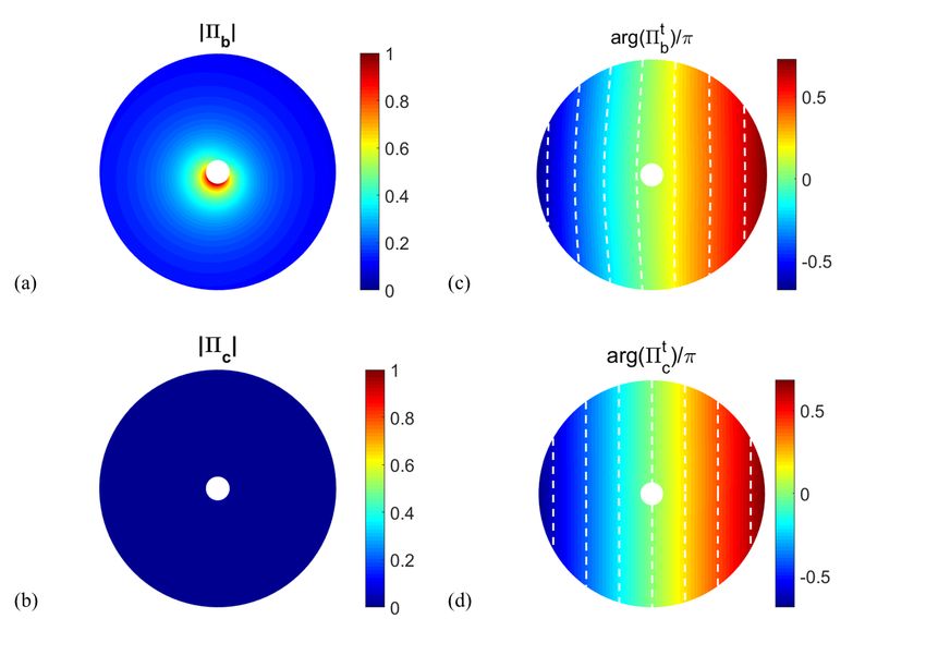
At this stage, one will derive the general equation for any properties of the rotating object,
and later, it will be assumed that ρ1 = ρ0 and κ1 = κ0 to single out the pure effects due to
spinning. An acoustic plane-wave of amplitude 1 is incident on the structure. For simplicity
and without loss of generality, let us assume that the wave is in the x − y plane, and that
it propagates in the x-direction. It can thus be expressed as pinc = eiβ0 x = eiβ0 r cos θ , by
ignoring the time-harmonic dependence, for now. The expansion of this incident plane wave
in terms of Bessel functions takes the form
                                                 +∞
                                                 X
                                       inc
                                   p         =        in Jn (β0 r) einθ .                     (5)
                                                 −∞

The scattered field is expanded in terms of Hankel functions of the first kind, to ensure that
the Sommerfield radiation condition is satisfied, i.e.
                                             +∞
                                             X
                                 pscat =           in sn Hn(1) (β0 r) einθ ,                  (6)
                                             −∞

for r > r1 and with sn the scattering coefficients to be determined using the boundary
conditions at the interfaces of the structure. Hence, the field in region 0 is p0 = pinc + pscat .
These scattering coefficients intervene in the definition of the scattering amplitude f (θ) ∝
√
  r limx→∞ pscat (r, θ), which is a measure of the acoustic scattering strength in the direction
θ. The total scattering cross-section (SCS) is the integration over all angles θ of the scattering
amplitude and represents a scalar measure of the total scattering (irrespective of direction),
and in the two-dimensional (2D) scenario is proportional to a length. For instance, one has
                                                         +∞
                                                      4 X
                                         σ scat =           |sn |2 .                          (7)
                                                      β0 −∞

To complete the expansion of the pressure fields, one considers now the case of the spinning
disc of radius r1 that is different from scattering objects that were considered in previous
studies, so far. In this case and owing to the previous results, the pressure field in the region
r ≤ r1 is given by
                                             +∞
                                             X
                                  p1 =            in an Jn (βn,1 r) einθ ,                    (8)
                                             −∞

with βn,1 given in Eq. (3) and an unknown coefficients to be determined by the boundary
conditions along with sn . Now by equating the pressure and the displacement [See Eq. (4)]
at the boundary r = r1 , i.e.

                                                      6
pinc (r1 ) + pscat (r1 ) = p1 (r1 ) ,
2Ω21 − ζn,1
2
1 ∂ pinc + pscat ∂r p1 − 3iζn,1 Ω1 np1 /r
= 2 . (9)
ρ0 ω 2 ∂r 2
ρ1 4Ω21 + ζn,1 2
Ω1 + ζn,1
r=r1 r=r1
Equation (9) yields with the previous expansions a set of linear systems, for each azimutal
order n, thanks to the orthogonality of the functions einθ , i.e.
(1)
Jn (βn,1 r1 ) −Hn (β0 r1 ) an Jn (β0 r1 )
= , (10)
β0 (1)0 β0 0
ΠJn − ω2 ρ0 Hn (β0 r1 ) sn J (β0 r1 )
ω 2 ρ0 n
where the coefficient ΠJn is expressed as
βn,1 Jn0 (βn,1 r1 ) − 3ζn,1r1Ω1 in Jn (βn,1 r1 )
2Ω21 − ζn,1
2
ΠJn = 2 . (11)
ρ1 4Ω21 + ζn,1 2
Ω1 + ζn,12
Equation (11) shows clearly for the specific case of scattering from spinning objects, that
the multipoles of orders n and −n give different contributions. The scattering coefficient sn
can be easily obtained from Eq. (10), i.e.
−1
(1)
Jn (βn,1 r1 ) Jn (β0 r1 ) Jn (βn,1 r1 ) −Hn (β0 r1 )
sn = (1)0
, (12)
β0
ΠJn J0
ω 2 ρ0 n
(β0 r1 ) ΠJn − ωβ20ρ0 Hn (β0 r1 )
where |M | denotes the determinant of a matrix M .
In order to single out the effect of rotation on the scattering, one considers an object
with the same density and bulk modulus as the surrounding environment, i.e. ρ1 = ρ0 and
κ1 = κ0 . This leaves us with only the rotation angular velocity Ω1 of the object (r ≤ r1 ). A
scenario of interest is that of small objects compared to the sound wavelength, i.e. β0 r1
1
and βn,1 r1
1. The first multipole terms are thus given by
3iπ α12 (β1 r1 )2 4
s0 = + O (β1 r 1 ) ,
4 1 − α12
iπ α1 (β1 r1 )2
+ O (β1 r1 )4 ,
s±1 =
4 ±2 + α1
iπ α1 (β1 r1 )4
+ O (β1 r1 )6 ,
s±2 =
32 ∓2 + α1
f±n (α1 ) (β1 r1 )2n + O (β1 r1 )2n+2 .
s±n = (13)
In Eq. (13), f± denote functions of the variable α1 . The upper/lower sign in the second and
third lines correspond to the positive/negative coefficient, respectively. Also, O(·) denotes
7the Landau notation (of a function of the same order) [78]. It may be noted that, if the
angular rotation velocity of the fluid goes to zero, all the scattering orders sn vanish without
exception. A case of interest is that of small rotation angular velocity, so the denominators
in Eq. (13) are close to 1 and can be omitted, thus one has s0 ∝ α12 ω 2 , s±1 ∝ α1 ω 2 , and s±2 ∝
α1 ω 4 . In classical scattering from non-rotating acoustic objects (or 2D electromagnetism),
it is well known that the scattering cross-section is dominated by both the zeroth-order and
first-order, i.e. the monopole s0 and the dipole s1 [79]. However, from Eq. (13), one can
see that s0 /s±1 ∝ α1
1 and s±2 /s±1 ∝ ω 2
1. Hence, unlike for the case of acoustics
at rest [74], the SCS of spinning objects is dominated by the dipole terms s±1 . The higher
order terms scale as (β1 r1 )2n and do not contribute significantly to the scattering, although in
Eq. (11) one has terms proportional to n. However, the peculiar behavior of Bessel functions
makes the higher order multipoles negligible in the quasi-static limit.
Another interesting remark about scattering of spinning fluids can be immediately seen
upon inspection of Eq. (13). One can see that the scattering coefficients possess poles for
determined values of α1 . Namely, these are ω = ±Ω1 for s0 , ∓Ω1 /2 for s1,−1 and ±Ω1 /2 for
s2,−2 . Thus for these frequencies, resonant scattering may be observed. For instance,
scat π α12 (α12 + 4)
σ ≈ (β0 r1 ) 2 . (14)
2 (α12 − 4)
Figure. 2(a) plots these normalized scattering coefficients 4/β0 |sn |2 in logarithmic scale
versus frequency (in logarithmic scale, too) for a spinning object (made of water, as the
surrounding, and separated from it by a thin membrane), with Ω1 = 2π rad, of radius
r1 = 1 m, bulk modulus and density κ1 = κ0 = 2.22 GPa and ρ1 = ρ0 = 103 kg/m3 ,
respectively, for n = 0, ±1, ±2. These plots show that although the object has the same
physical parameters as the environment (water, here, for instance) resonant modes take
place at specific frequencies given by Eq. (13). It should be also noted that both modes
n = 0 and n = ±1 dominate, as can be anticipated from Eq. (13). Also the resonance
of modes n = 1 and n = −2 cannot be seen here as one uses positive Ω1 (= 2π rad).
Figure. 2(b) depicts the total scattering cross-section σscat with 21 scattering orders taken
into account (n = −10 : 10) versus the normalized spinning velocity for different kinds of
p
objects, ranging from soft, i.e. (κ1 ρ1 )/(κ0 ρ0 )
1 [green line in Fig. 2(b)] ”non-rigid”,
p
i.e. (κ1 ρ1 )/(κ0 ρ0 ) ≈ 1 [red and blue lines in Fig. 2(b)], to hard-wall (rigid) (detailed
p
in Section III C), i.e. (κ1 ρ1 )/(κ0 ρ0 )
1 [black dashed line in Fig. 2(b)]. The resonant
8scattering can be seen from all these objects around the predicted spinning velocities. Here the frequency is fixed at 1 Hz (quasistatic limit). It should be noted that the presence of these Mie resonances is unusual in acoustics, where homogeneous objects do not possess low frequency resonance. The only case of low-frequency Mie resonances, concerns flexural waves scattered off thin-plate objects as was analyzed in Ref. [80], originating from the peculiar nature of flexural biharmonic waves obeying a fourth order PDE [81]. However, in the present scenario, these resonances re due to pure rotation. Figure 2(c) plots contours of normalized SCS σ scat /r1 (in logarithmic scale) of a scatterer with the same physical properties as the surrounding (water) for varying frequencies ω and spinning speeds Ω1 . This plot clearly shows that the SCS has two resonances (marked with dark red color) for each spinning speed. Moreover, the blue horizontal thick linear region at the center with blue color (i.e. zero scattering) corresponds to very low down to zero spinning speeds, and as the scatterer possesses the same density and bulk modulus of the surrounding, it does not scatter at all at these low spinning speeds. On the other hand, if one takes vertical cuts along this 2D graph, four resonances occur (in a symmetric manner with respect to Ω1 ) as it transpires from Fig. 2(b) and as predicted from Eq. (13.) The inset of Fig. 2(c) plots the real part distribution of the pressure field [
and κ0 , as the fluid in region 0 is at rest. The field expansions are similar to the ones of a
bare object. However, one has now an additional domain (the shell) r1 < r ≤ r2 , where the
pressure field can be expanded as
+∞
X
p2 = in [bn Jn (βn,2 r) + cn Yn (βn,2 r)] einθ , (15)
−∞
q p
with Yn the Bessel function of second kind, βn,2 = 2
−(4Ω22 + ζn,2 )/c22 and c2 = κ2 /ρ2 .
The obtained scattering system for this structure is thus obtained by applying the same
boundary conditions at the interfaces r = r1 and r = r2 , taking into account that the fluid
is either rotating or at rest. This leads to
(1)
0 Jn (βn,2 r2 ) Yn (βn,2 r2 ) −Hn (β0 r2 ) an Jn (β0 r2 )
(1)0
β0 β0 0
0 ΠJn (β r
n,2 2 ) ΠYn (β r
n,2 2 ) − H
ω 2 ρ0 n
(β r ) b
0 2 n
J (β r
ω 2 ρ0 n 0 2 )
= ,
−Jn (βn,1 r1 ) Jn (βn,2 r1 ) Yn (βn,2 r1 ) 0 cn 0
−ΠJn (βn,1 r1 ) ΠJn (βn,2 r1 ) ΠYn (βn,2 r1 ) 0 sn 0
(16)
with the functionals ΠYn given in the same way as ΠJn , shown in Eq. (11), up to the
replacement of Jn by Yn . The scattering coefficient is thus sn = |M |/|M̃ |, where M is the 4×4
matrix in the LHS of Eq. (16) and M̃ is the matrix obtained from M by replacing its fourth
column vector by the vector in the RHS of Eq. (16). Solving Eq. (16) is straightforward using
a numerical software such as Matlab [82], and this will be performed later to characterize
and analyze this peculiar cloaking mechanism.
B. Analysis of the SCT
In order to gain more insight, and due to the general complexity of this linear system,
it is instructive to analyze the long wavelength limit (as done for the bare object in pre-
vious section) corresponding to acoustically small objects and shells, i.e. β0 r1,2
1 and
βn,1,n,2 r1,2
1. Note that with the values of the parameters in this study, it is suffi-
cient to impose the first condition β0 r1
1. Under these assumptions, and by denoting
Ω1 = α1 ω, Ω2 = α2 ω, r2 = r1 /γ, and by choosing without loss of generality ρ2 = ρ1 = ρ0
and c2 = c1 = c0 , in order to single out the effect of spinning (by ignoring scattering due
10to the acoustic impedance mismatch due to inhomogeneities), one obtains for the leading
scattering orders, as discussed in the previous sub-section,
3iπ [γ 2 α12 − (−1 + γ 2 + α12 ) α1 α2 ]
s0 = (β0 r1 )2
4γ 2 (−1 + α12 ) (−1 + α1 α2 )
+ O (β0 r1 )4 ,
(17)
and
iπ A±1 2 3
s±1 = (β0 r 1 ) + O (β 0 r1 ) , (18)
4γ 2 B±1
with
A±1 = ±2γ 2 α1 + α2 ±2 ∓ 2γ 2 + α1 − 6γ 2 α1
+ α22 −3 + 6γ 2 ± α1 ± 4γ 2 α1
+ α23 ±1 ∓ 4γ 2 + 6γ 2 α1 + α24 6 1 − γ 2 ,
(19)
and
B±1 = 4 ± 2α1 + α2 ∓4 + 3α1 − 2γ 2 α1
+ α22 −1 + 2γ 2 ± α1 ∓ 2γ 2 α1
+ α23 ±13 ± 2γ 2 + 6γ 2 α1 + α24 6 1 − γ 2 .
(20)
In Eqs. (19)-(20) the upper (lower) sign correspond to the order n = 1 (n = −1). Note
that as α2 → 0 i.e. the shell is at rest, the expressions of s0 and s±1 given in Eqs. (17)-(20)
reduce to the ones given in Eq. (13), as expected.
In order to cancel the total SCS, i.e. σ scat , one has to enforce s0 = 0 and s±1 = 0. For
small angular rotation speeds, only s±1 is significant (as one has seen earlier from Eq. (13)).
and it is safe to ignore the contribution of the higher order multipoles (|n| ≥ 2), as these
scale with (β0 r1 )2n (their squared amplitude, i.e. their contribution to the SCS, from Eq. (7)
scales with (β0 r1 )4n−1 , which is even smaller).
First, enforcing |s0 | = 0, one derives the quasistatic condition of SCT, i.e.
γ 2 α12 − (−1 + γ 2 + α12 )α22 = 0 , (21)
which relates α2 , α1 , r1 , and r2 (via γ). It is found that, to satisfy Eq. (20), α2 must take
positive and/or negative values. Note that positive (resp. negative) angular velocity just
means an anticlockwise (resp. clockwise) rotation. One thus has
γα1
α2 = ± p . (22)
(−1 + γ 2 + α12 )
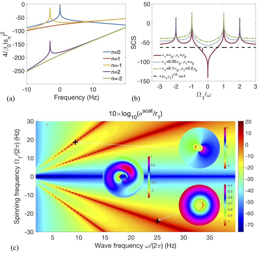
11Also, when γ 2 +α12 ≤ 1, no solution can be abtained, that may cancel the scattering monopole
s0 . The behavior of α2 , versus γ and α1 , corresponding to Eq. (17) is depicted in Fig. 3(a).
Specifically, one can observe that for the domain γ 2 + α12 ≤ 1, no solution for α2 can be
obtained (empty region of the plot). For γ 2 + α12 = 1, very high positive (and negative)
values of α2 are required. On the other hand, when the condition on γ 2 + α12 is relaxed,
small values of α2 are sufficient. It should be also noted that α2 is symmetric with respect
to the variation of α1 (α1 and −α1 give the same values of α2 ) as seen from Fig. 3(a).
Let us now turn to the analysis of cancelling the leading scattering dipole orders s±1 .
In fact, Eq. (19) is of fourth order, so one may expect to obtain four distinct solutions
for α2 . This is exactly what may be observed in Fig. 3(b), where four branches can be
distinguished in this three-dimensional contourplot. In this scenario, one can see that there
is a lack of symmetry with respect to α1 , due to the presence of the dipole order term
in the equation (n = ±1). Clockwise an anti-clockwise rotations Ω2 are thus viable ways
to counteract the anti-clockwise rotation of the object and make it look static to external
observers (by cancelling the n = ±1 multipoles). The angular rotation speeds needed here
are also comparable to the speed of the object to cancel. The graphs of Fig. 3 are only
dependent of frequency through the parameters αi = Ωi /ω.
Next, one considers the general case where one does not make use of asymptotic (qua-
sistatic) approximation, and solve the exact scattering problem, stemming from Eq. (16).
The angular rotation speed of the fluid in region 1 (r ≤ r1 ) is Ω1 /(2π) = 15 Hz and its den-
sity and bulk modulus are assumed, as before, equal to those of free-space (water). Here, the
frequency of the wave is chosen as ω/(2π) = 16.75 Hz (high spinning regime, i.e. Ω1 ≈ ω).
σcscat of the total object-shell structure is normalized with the SCS of the bare object and
subsequently plotted against varying values of Ω2 (in units of 2π rad) and γ. This result
is shown in Fig. 4(a) in logarithmic scale. The regions colored with dark blue correspond
to significant scattering reduction (i.e. σcscat /σbscat
1), whereas red regions correspond to
enhanced scattering from the core-shell geometry. it can be seen that two distinct regions
of cloaking can be distinguished, i.e. for γ > 0.6 and for γ ≈ 0.3, and both with values of
Ω2 /(2π) between -30 Hz and -10 Hz. In particular, a minimum of -30 dB of σcscat /σbscat
1
is seen around values of Ω2 /(2π) = −20 Hz and γ = 0.65.
To isolate the effect of Ω2 and γ on the scattering reduction mechanism, a plot of
σcscat /σbscat
1 is given versus Ω2 /(2π) for different values of γ in Fig. 4(c). One can
12see that one single scattering dip exists for some values of γ. For instance for γ = 0.45; 0.99,
no cloaking is possible. The minimum cloaking is for Ω2 = −20 Hz and γ = 0.65. Next,
σcscat /σbscat
1 is plotted versus γ and for different values of Ω2 /(2π). One can see that here
two cloaking regimes take place. First, for small values of γ around 0.3, a small reduction
of the range of -16 dB can be observed for an extended range of Ω2 /(2π). Then, for higher
values of γ, i.e. γ ≥ 0.6, an efficient scattering reduction regime takes place (more than -20
dB). This second cloaking dip is more sensitive to changes of Ω2 , in comparison to the first
one, where a redshift can be clearly observed.
To better illustrate the efficiency of the proposed cloak, the far-field scattering patterns
(i.e. |f (θ)|) in polar coordinates is shown in Fig. 4(b), for two specific parameters of Ω2
and γ, depicted in Fig. 4(d) with circles. This plot demonstrates that the spinning fluid is
undetectable for all angles [Fig. 4(c) gives ormalized |fc (θ)/fb (θ)|, with subscripts c and b,
denoting, as before, the cloaked and bare object, respectively]. It can be seen also that the
high γ regime (solid curve) gives better angular SCS reduction than the γ ≈ 0.3 regime,
and confirms that an a clockwise rotating shell of small radius can cloak an anti-clockwise
spinning object.
Last, Figs. 5(a)-(b) plot the near-field scattered pressure field amplitude (or more precisely
the amplitude of the normalized scattered acoustic Poynting vector [83] , i.e. |Πb | and /|Πc |)
in the environment region (region 0) for the bare object and cloaked object, respectively.
One can see that a drastic reduction of the scattered fields (about two orders of magnitude),
takes place, in the case of an object with spinning coating. The phases (normalized with π)
of the total Poynting vectors are given in Fig. 5(c) and Fig. 5(d) for the bare and cloaked
object with same parameters as in Fig. 5(a) and Fig. 5(b), respectively. These plots show
that the phase of the fields is not distorted in the case of cloaked scenario (straight contour
lines, marked with the dashed white lines) whereas for the bare case it is slightly distorted
(contour lines are curved due to the enhanced scattering from the spinning object).
C. The Case of a Hard-Wall Object
Let us first derive the equivalence of the scattering from a hard-wall object and an infinite
acoustic impedance object. The hard-wall (rigid) boundary condition for r = r1 , namely
n · v = 0 (or in terms of pressure 1/ρ ∂r p = 0.) The incident field is as usual a plane-wave
13expressed as in Eq. (5) and the scattered pressure is given as in Eq. (6). By application of
the hard-wall boundary condition at r1 , one obtains the expression of the coefficients
−Jn0 (β0 r1 )
s(r)
n = (1)0
, ∀n ∈ Z . (23)
Hn (β0 r1 )
On the other hand, an object of same radius r1 , density ρ1 , and bulk modulus κ1 embedded
in a homogeneous medium of density ρ0 and bulk modulus κ0 , possesses scattering given by
−1
(1)
Jn (β1 r1 ) Jn (β0 r1 ) Jn (β1 r1 ) Hn (β0 r1 )
sn = (1)0
, (24)
Jn0 (β1 r1 ) χJn0 (β0 r1 ) Jn0 (β1 r1 ) χHn (β0 r1 )
√
where χ = Z1 /Z0 , and Z0,1 = ρ0,1 κ0,1 the impedance of the object and free-space, respec-
tively.
Now in order to establish the analogy between the hard-wall boundary and the inhomo-
geneous medium, one must equalize Eqs. (23)-(24). This can be obtained for all scattering
orders, if one ensures that χ → ∞, i.e. by assuming an infinite impedance of the object.
This is is somehow coherent as the higher impedance leads to enhanced reflection and in this
limit the fields cannot penetrate the object, which is an equivalent to hard-wall boundary.
This fact is demonstrated in Fig. 6(a), where the plot of the SCS versus a broadband of
frequencies is depicted. It can be also seen from Fig. 6(a) that rotating a hard-wall object
does not change its scattering response, unlike for the case of an acoustic medium with finite
impedance. This is mainly due to the fact that there is no flow inside the object (pressure
and velocity are zero for r ≤ r1 ) and hence rotating the object does not induce any extra
scattering features.
Last, to verify the versatility and robustness of this new kind of SCT-based cloaking, one
investigates the possibility to cloak a rigid (hard-wall like) cylindrical object by using only a
rotating shell, of same physical parameters (ρ2 and κ2 ) as those of the surrounding medium
(water, here). The rigid body can mimic for example a submarine, or any under-water solid
(one ignores shear waves here, as only compression waves are investigated). One first coats
the rigid object of radius r1 = 1 with a shell of radius r2 = 1.2 and one sweeps the density
and bulk modulus of the shell, as usually done in SCT cloaking. The normalized SCS is
plotted as before, at frequency ω/(2π) = 360 Hz, and the result is depicted in Fig. 6(b). On
the other hand, one considers to coat the same object with a shell of radius r2 = r1 /γ and
spinning angular frequency Ω2 . In this scenario ρ2 = ρ0 and κ2 = κ0 . So the SCT is induced
14here purely by spinning effect. The result is depicted in Fig. 6(c) and it can be clearly
seen that comparable scattering cancellation is possible to achieve. The advantage is here
that one does not need near-zero or negative density and/or bulk modulus for the cloaking
operation [as can be seen from Fig. 6(b)]. By pure rotation of homogeneous shells, cloaking
is made possible. Note one can further improve this scattering rotation with spinning by
allowing some freedom for the density and/or bulk modulus of the shell.
IV. CONCLUDING REMARKS
In summary, a detailed analysis of spinning acoustic objects and their scattering prop-
erties is proposed, and acoustic cloaks based on the scattering cancellation technique are
designed. Here the main challenge is that the object to conceal (cloak) is not at rest,
and experiences rotation along its z-axis (for cylinders) at constant angular speed (with a
few rotation cycles per second). Scattering by such acoustic rotating objects is physically
different from objects at rest, and possesses resonant Mie features at specific frequencies.
The cloaking mechanism introduced here presents several advantages in comparison with
zero-velocity cloaking, as it may be more useful in realistic applications (where objects are
most of the time moving). Using a homogeneous layer of same properties as free-space with
a rotation (in the opposite direction to the object) one is able to significantly reduce the
scattering from objects with various spinning speeds. It is also shown that using purely a
spinning shell, it is possible to cancel the scattering from a rigid (hard-wall) object in a
similar manner as optimizing its density and bulk modulus, which shows the versatility of
this cloaking mechanism.
Experimental realization of this concept may be within reach readily, as it only requires
rotating objects and shells, allowing for interesting applications in scenarios in which it is
desirable to suppress the scattering from obstacles that are in a spinning movement (e.g.
rotating components of cars or helicopter rotor blades) for noise reduction. The same concept
can also be generalized to other classes of waves, such as linear surface water waves, flexural
waves in thin-plates or beams.
15Acknowledgements
The research reported in this manuscript was supported by Baseline Research Fund
BAS/1/1626-01-01.
Appendix A: Derivation of The Acoustic Equation in Spinning Media
Let us consider a uniformly rotating medium, as schematized in Fig. 1(a). The usual
equations of motion (momentum conservation) and continuity (conservation of mass) need
be modified [55–58, 61, 77]. If one considers no shear stresses and body forces, it is shown
that the momentum conservation can be written as,
Du
ρ = −∇0 P , (A1)
Dt0
where the operators D/Dt0 and ∇0 represent the total time-derivative and the spatial deriva-
tive, respectively, in the reference frame R0 associated with the spinning disc. The density
ρ is assumed to be constant with respect to time, due to low compressibility and reasonable
rates of rotation, as well as small-amplitude sound waves, as usually assumed. Here the
total pressure P accounts for the pressure due to acoustic waves as well as to the rotation
of the structure and u is the total velocity.
In the reference frame R associated with the laboratory, Eq. (A1) is transformed into
∂
ρ + (u · ∇) u = −∇P , (A2)
∂t
with u = u0 + v, with v the velocity of the acoustic wave, and u0 = u0 (r) the bulk velocity,
that corresponds to rotation. For a uniform spinning, one has u0 = Ωreθ , with eθ the
azimutal unit-vector and Ω the angular velocity. By denoting P = p0 + p, with p0 the
time-independent pressure due to the frame motion and p the pressure of the acoustic waves
(due to the acoustic perturbation). Equation (A2) can be expressed as [77]
∂
+ (u0 · ∇) v + (v · ∇) · u0 = −ρ−1 ∇p . (A3)
∂t
For the mass conservation equation, a similar reasoning permits to show that it can be
expressed in the laboratory frame R as
∂
+ (u0 · ∇) p + c2 ρ∇ · v = 0 , (A4)
∂t
16p
using the fact that ∇ · u0 = 0 and noting c = κ/ρ, with κ the bulk modulus of the
structure.
Similarly, the boundary conditions at the interface between two spinning media (or a
spinning media and a medium at rest) shall be modified [77]. For instance, the pressure p
is continuous across the interface. For the second boundary condition, that is the normal
component of the velocity (n·v), in media at rest, it was shown in Ref. [77] that it should be
replaced in the moving media by the displacement ψ, that is related to the pressure through
the modified relation
∂ ∂ ∂p
ρ + vn1 ψn2 = − , (A5)
∂t ∂n1 ∂n2
with vn1 = v · n1 and ψn2 = Ψ · n2 , where n1 is the direction of the flow velocity and n2 is
the normal to the considered interface. It is also assumed here that a very thin membrane
separates both fluids from mixing, and that the spinning of both fluids is thus independent.
[1] E. Yablonovitch, Physical review letters 58, 2059 (1987).
[2] S. John, Physical review letters 58, 2486 (1987).
[3] R. Meade, J. N. Winn, and J. Joannopoulos, Photonic crystals: Molding the flow of light
(1995).
[4] H. Benisty, V. Berger, J.-M. Gerard, D. Maystre, and A. Tchelnokov, Photonic crystals:
Towards nanoscale photonic devices (Springer, 2008).
[5] J. Knight, T. Birks, P. S. J. Russell, and D. Atkin, Optics letters 21, 1547 (1996).
[6] P. Russell, science 299, 358 (2003).
[7] T. White, B. Kuhlmey, R. McPhedran, D. Maystre, G. Renversez, C. M. De Sterke, and
L. Botten, JOSA B 19, 2322 (2002).
[8] F. Zolla, G. Renversez, A. Nicolet, B. Kuhlmey, S. Guenneau, D. Felbacq, A. Argyros, and
S. G. Leon-Saval, Foundations of photonic crystal fibres.
[9] M. S. Kushwaha, Applied Physics Letters 70, 3218 (1997).
[10] J. Vasseur, P. A. Deymier, G. Frantziskonis, G. Hong, B. Djafari-Rouhani, and L. Dobrzynski,
Journal of Physics: Condensed Matter 10, 6051 (1998).
[11] Y. Tanaka and S.-i. Tamura, Physical Review B 58, 7958 (1998).
[12] Y. Tanaka, Y. Tomoyasu, and S.-i. Tamura, Physical Review B 62, 7387 (2000).
17[13] X. Zhang and Z. Liu, Applied Physics Letters 85, 341 (2004).
[14] Z. Yang, J. Mei, M. Yang, N. Chan, and P. Sheng, Physical review letters 101, 204301 (2008).
[15] Z. Liang, M. Willatzen, J. Li, and J. Christensen, Scientific reports 2, 859 (2012).
[16] S. Yang, J. H. Page, Z. Liu, M. Cowan, C. T. Chan, and P. Sheng, Physical review letters 88,
104301 (2002).
[17] Y. Pennec, B. Djafari-Rouhani, J. Vasseur, A. Khelif, and P. A. Deymier, Physical Review E
69, 046608 (2004).
[18] L.-W. Cai and J. Sánchez-Dehesa, The Journal of the Acoustical Society of America 124,
2715 (2008).
[19] M. Amin, A. Elayouch, M. Farhat, M. Addouche, A. Khelif, and H. Bağcı, Journal of Applied
Physics 118, 164901 (2015).
[20] S. A. Cummer, J. Christensen, and A. Alù, Nature Reviews Materials 1, 16001 (2016).
[21] M. Landi, J. Zhao, W. E. Prather, Y. Wu, and L. Zhang, Physical review letters 120, 114301
(2018).
[22] Y. Wu, M. Yang, and P. Sheng, Journal of Applied Physics 123, 090901 (2018).
[23] B. Assouar, B. Liang, Y. Wu, Y. Li, J.-C. Cheng, and Y. Jing, Nature Reviews Materials 3,
460 (2018).
[24] P. A. Deymier, Acoustic metamaterials and phononic crystals, vol. 173 (Springer Science &
Business Media, 2013).
[25] R. V. Craster and S. Guenneau, Acoustic metamaterials: Negative refraction, imaging, lensing
and cloaking, vol. 166 (Springer Science & Business Media, 2012).
[26] Z. Liu, C. T. Chan, and P. Sheng, Physical Review B 71, 014103 (2005).
[27] F. di Cosmo, M. Laudato, and M. Spagnuolo, in Generalized Models and Non-classical Ap-
proaches in Complex Materials 1 (Springer, 2018), pp. 247–274.
[28] J. B. Pendry, A. Holden, W. Stewart, and I. Youngs, Physical review letters 76, 4773 (1996).
[29] J. B. Pendry, A. J. Holden, D. J. Robbins, and W. Stewart, IEEE transactions on microwave
theory and techniques 47, 2075 (1999).
[30] J. B. Pendry, Physical review letters 85, 3966 (2000).
[31] D. R. Smith, W. J. Padilla, D. Vier, S. C. Nemat-Nasser, and S. Schultz, Physical review
letters 84, 4184 (2000).
[32] Z. Liu, X. Zhang, Y. Mao, Y. Zhu, Z. Yang, C. T. Chan, and P. Sheng, science 289, 1734
18(2000).
[33] J. Li and C. T. Chan, Physical Review E 70, 055602 (2004).
[34] G. Papanicolaou, Wave propagation in complex media, vol. 96 (Springer Science & Business
Media, 2012).
[35] M. Farhat, P.-Y. Chen, S. Guenneau, and S. Enoch, Transformation wave physics: electro-
magnetics, elastodynamics, and thermodynamics (CRC Press, 2016).
[36] M. Farhat, P.-Y. Chen, H. Bağcı, S. Enoch, S. Guenneau, and A. Alu, Scientific reports 4,
4644 (2014).
[37] S. Brûlé, S. Enoch, and S. Guenneau, Physics Letters A 384, 126034 (2020).
[38] M. Farhat, S. Enoch, S. Guenneau, and A. Movchan, Physical review letters 101, 134501
(2008).
[39] G. Dupont, O. Kimmoun, B. Molin, S. Guenneau, and S. Enoch, Physical Review E 91,
023010 (2015).
[40] J. Park, J. R. Youn, and Y. S. Song, Physical review letters 123, 074502 (2019).
[41] S. Zou, Y. Xu, R. Zatianina, C. Li, X. Liang, L. Zhu, Y. Zhang, G. Liu, Q. H. Liu, H. Chen,
et al., Physical review letters 123, 074501 (2019).
[42] J. B. Pendry, D. Schurig, and D. R. Smith, science 312, 1780 (2006).
[43] U. Leonhardt, science 312, 1777 (2006).
[44] F. Zolla, S. Guenneau, A. Nicolet, and J. Pendry, Optics Letters 32, 1069 (2007).
[45] W. F. Bahret, IEEE Transactions on Aerospace and Electronic Systems 29, 1377 (1993).
[46] T. R. Neil, Z. Shen, D. Robert, B. W. Drinkwater, and M. W. Holderied, Journal of the Royal
Society Interface 17, 20190692 (2020).
[47] W. Cai, U. K. Chettiar, A. V. Kildishev, and V. M. Shalaev, Nature photonics 1, 224 (2007).
[48] M. Farhat, S. Guenneau, A. Movchan, and S. Enoch, Optics express 16, 5656 (2008).
[49] T. Ergin, N. Stenger, P. Brenner, J. B. Pendry, and M. Wegener, science 328, 337 (2010).
[50] A. Alù and N. Engheta, Physical Review E 72, 016623 (2005).
[51] P.-Y. Chen, J. Soric, and A. Alu, Advanced Materials 24, OP281 (2012).
[52] H. Chen and C. Chan, Applied physics letters 91, 183518 (2007).
[53] G. Dupont, M. Farhat, A. Diatta, S. Guenneau, and S. Enoch, Wave Motion 48, 483 (2011).
[54] J. Xu, X. Jiang, N. Fang, E. Georget, R. Abdeddaim, J.-M. Geffrin, M. Farhat, P. Sabouroux,
S. Enoch, and S. Guenneau, Scientific reports 5, 1 (2015).
19[55] E. Graham and B. Graham, The Journal of the Acoustical Society of America 46, 169 (1969).
[56] D. Censor and J. Aboudi, Journal of Sound and Vibration 19, 437 (1971).
[57] M. Schoenberg and D. Censor, Quarterly of Applied Mathematics 31, 115 (1973).
[58] D. Censor and M. Schoenberg, Applied Scientific Research 27, 401 (1973).
[59] P. Peng, J. Mei, and Y. Wu, Physical Review B 86, 134304 (2012).
[60] M. P. Lavery, F. C. Speirits, S. M. Barnett, and M. J. Padgett, Science 341, 537 (2013).
[61] S. Farhadi, Journal of Sound and Vibration 428, 59 (2018).
[62] D. Ramaccia, D. L. Sounas, A. Alù, A. Toscano, and F. Bilotti, IEEE Transactions on An-
tennas and Propagation (2019).
[63] Y. Mazor and B. Z. Steinberg, Physical Review Letters 123, 243204 (2019).
[64] D. Zhao, Y.-T. Wang, K.-H. Fung, Z.-Q. Zhang, and C. Chan, Physical Review B 101, 054107
(2020).
[65] B. Z. Steinberg, A. Shamir, and A. Boag, Physical Review E 74, 016608 (2006).
[66] R. Novitski, B. Z. Steinberg, and J. Scheuer, Optics express 22, 23153 (2014).
[67] B. Z. Steinberg, Physical Review E 71, 056621 (2005).
[68] B. Z. Steinberg and A. Boag, JOSA B 24, 142 (2007).
[69] D. Ramaccia, D. L. Sounas, A. Alù, A. Toscano, and F. Bilotti, Phys. Rev. B 95, 075113
(2017).
[70] D. Ramaccia, D. L. Sounas, A. Alù, F. Bilotti, and A. Toscano, IEEE Antennas and Wireless
Propagation Letters 17, 1968 (2018).
[71] M. W. McCall, A. Favaro, P. Kinsler, and A. Boardman, Journal of optics 13, 024003 (2010).
[72] M. Fridman, A. Farsi, Y. Okawachi, and A. L. Gaeta, Nature 481, 62 (2012).
[73] M. D. Guild, M. R. Haberman, and A. Alù, The Journal of the Acoustical Society of America
128, 2374 (2010).
[74] M. Farhat, P.-Y. Chen, S. Guenneau, S. Enoch, and A. Alu, Physical Review B 86, 174303
(2012).
[75] R. Fleury and A. Alù, Physical Review B 87, 045423 (2013).
[76] M. Farhat, P.-Y. Chen, S. Guenneau, H. Bağcı, K. N. Salama, and A. Alu, Proceedings of the
Royal Society A: Mathematical, Physical and Engineering Sciences 472, 20160276 (2016).
[77] P. M. Morse, Princeton University Press, 949p 4, 150 (1968).
[78] E. Landau, Handbuch der Lehre von der Verteilung der Primzahlen, vol. 1 ( , 2000).
20[79] Y. Wu, J. Li, Z.-Q. Zhang, and C. Chan, Physical Review B 74, 085111 (2006).
[80] M. Farhat, P.-Y. Chen, S. Guenneau, K. N. Salama, and H. Bağcı, Physical Review B 95,
174201 (2017).
[81] K. F. Graff, Wave motion in elastic solids (Courier Corporation, 2012).
[82] Matlab, R2019a, URL https://www.mathworks.com/.
[83] C. Tang and G. A. McMechan, Geophysics 83, S365 (2018).
21FIG. 1: (a) Real and (b) imaginary parts of the spinning wavenumbers for different orders n versus
the rotation coefficient α1 = Ω1 /ω. The inset of (a) plots the scheme of the multiple layers and
the interfaces of an acoustic structure, as well as the rotation directions.
22FIG. 2: (a) Scattering coefficients 4/β0 |sn |2 in logarithmic scale versus frequency (in logarithmic
scale, too) for a spinning object (Ω1 /(2π) = 1 Hz) of radius r1 = 1 m, bulk modulus and density
κ1 = κ0 = 2.22 GPa and ρ1 = ρ0 = 103 kg/m3 , respectively, for n = 0, ±1, ±2. (b) Total normalized
SCS (σ scat /r1 ) with 21 scattering orders taken into account (n = −10 : 10) versus the normalized
√ √
spinning velocity for different kinds of objects, ranging from soft ( κ1 ρ1
1), ”normal” ( κ1 ρ1 ≈
√
1), to hard-wall (See Section III C) ( κ1 ρ1
1). (c) Normalized SCS in logarithmic scale, of the
spinning cylinder vs the frequency of the acoustic wave ω and the spinning velocity Ω1 for the
same physical parameters as the environment (water). The inset plotsFIG. 3: (a) Contour plot of α2 versus α1 and γ for the first order (n = 0) condition, given in
Eq. (17). (b) Contour plot of α2 versus α1 and γ for the second order condition (n = ±1), given
in Eqs. (18)-(20).
24FIG. 4: (a) Normalized SCS (σcscat /σbscat ) in logarithmic scale, (where the subscripts c and b refer to
the scattering cross-section of the obstacle and cloaked structure, respectively) versus the spinning
frequency of the cloaking shell Ω2 /(2π) and the ratio γ. The highlighted region represents the
locations of optimized scattering reduction, with a value exceeding 30 dB. The inset gives the
acoustic Poynting vector of the cloaked structure normalized by the one of the bare object in the
scattering region. (b) Scattering amplitude (|f (θ)|2 ) in logarithmic scale for the cloaked structure
(normalized by the amplitude of the bare object) for Ω2 /(2π) = −20 Hz two different radii of the
cloak, corresponding to the highlighted values from (d). (c) Normalized SCS versus the spinning
frequency of the cloaking shell Ω2 /(2π) for various values of γ. (d) Normalized SCS versus γ for
various values of Ω2 /(2π). All these figures were plotted for a frequency of ω/(2π) = 16.75 Hz and
Ω1 /(2π) = 15 Hz.
25FIG. 5: (a) Near-field plot (in arbitrary units) of the acoustic scattered Poynting vector Πb (pro-
portional to |pscat |2 ) of the bare object of radius r1 = 1 m, spinning with speed Ω1 /(2π) = 15 Hz
at the frequency ω/(2π) = 16.75 Hz. (b) Same as in (a) for the cloaked object (Πc ), with the
shell of radius r2 = r1 /γ and γ = 0.65 and spinning frequency Ω2 /(2π) = −20 Hz. The physical
parameters of the object and shell are equal to those of the surrounding, i.e., water. The phases
(normalized with π) of the total Poynting vectors are given in (c) and (d) for the bare and cloaked
object with same parameters as in (a) and (b), respectively. The white dashed lines represent the
contours of the phases.
26FIG. 6: (a) SCS for the hard-wall boundary (blue line), infinite acoustic impedance approxima-
√
tion, i.e., ρ1 κ1 → ∞ (red dashed line), and spinning infinite acoustic impedance approximation
(circles). (b) Cloaking scenario for the hard-wall object of radius r1 = 1 when using classical SCT
scheme, i.e., by varying the density and bulk modulus of the shell of radius r2 = 1.2 at frequency
ω/(2π) = 360 Hz. (c) Same as in (b) but using a spinning shell of density and bulk modulus equal
those of free-space.
27You can also read