Towards bio inspired artificial muscle: a mechanism based on electro osmotic flow simulated using dissipative particle dynamics

Page created by Dan Wang
 
CONTINUE READING
Towards bio inspired artificial muscle: a mechanism based on electro osmotic flow simulated using dissipative particle dynamics
www.nature.com/scientificreports

                OPEN             Towards bio‑inspired artificial
                                 muscle: a mechanism based
                                 on electro‑osmotic flow simulated
                                 using dissipative particle dynamics
                                 Ramin Zakeri
                                 One of the unresolved issues in physiology is how exactly myosin moves in a filament as the smallest
                                 responsible organ for contracting of a natural muscle. In this research, inspired by nature, a model
                                 is presented consisting of DPD (dissipative particle dynamics) particles driven by electro-osmotic
                                 flow (EOF) in micro channel that a thin movable impermeable polymer membrane has been attached
                                 across channel width, thus momentum of fluid can directly transfer to myosin stem. At the first,
                                 by validation of electro-osmotic flow in micro channel in different conditions with accuracy of less
                                 than 10 percentage error compared to analytical results, the DPD results have been developed to
                                 displacement of an impermeable polymer membrane in EOF. It has been shown that by the presence
                                 of electric field of 250 V/m and Zeta potential − 25 mV and the dimensionless ratio of the channel
                                 width to the thickness of the electric double layer or kH = 8, about 15% displacement in 8 s time
                                 will be obtained compared to channel width. The influential parameters on the displacement of the
                                 polymer membrane from DPD particles in EOF such as changes in electric field, ion concentration, zeta
                                 potential effect, polymer material and the amount of membrane elasticity have been investigated
                                 which in each cases, the radius of gyration and auto correlation velocity of different polymer
                                 membrane cases have been compared together. This simulation method in addition of probably
                                 helping understand natural myosin displacement mechanism, can be extended to design the
                                 contraction of an artificial muscle tissue close to nature.

                                 The state of the art. Undoubtedly, one of essential issues in nature is the movement of living organisms
                                  in the sea, land and air. Muscle contractions are responsible for causing this ­displacement1. How muscles con-
                                 tract in the deepest layer, are almost entirely related to the contraction of micro filaments and within micro-
                                 filaments are associated to the two vital organs myosin and actin. The most important part of the contraction
                                 depends on the movement of myosins, which they act like the movement of paddles and causes wavy movements
                                 and contraction in a microfilaments is formed. Combinations of these movements provide fiber and muscle
                                 ­contraction1–3. The movement of myosin probably originates from the release of calcium ions, fluid transfer, and
                                 the release of energy, which is caused the swelling of thin membrane and motion of myosin should be formed
                                 while exactly mechanism of myosin motion is one of the unknowns in physiology. Based on the valid sliding
                                 theory of muscle contraction, with angular movement of a myosin, the filament contraction will be occurred
                                 and consequently contraction of fibers and muscles will be resulted considering the combination of series and
                                 parallel mechanism of ­filaments1,4,5.
                                      In order to imitate nature and fabrication of artificial muscles for providing a d ­ isplacement6, various works
                                  have been reported including ionic polymer metal c­ omposite7,8, dielectric e­ lastomer9, ionic conducting p
                                                                                                                                             ­ olymer10.
                                 These methods need high voltage to operate or the efficiency or mechanisms of these methods are not like a
                                 natural muscle c­ ontraction1. Also, the independent methods to high voltage such as shape memory a­ lloy11,
                                 molecular machines m   ­ otion12 or polyvinyl chloride g­ el13 need more time for reaction compared to real natural
                                  muscle. Due to the many limitations of the proposed methods compared to natural muscle contraction, there
                                  is a requirement to study a natural muscle more closely and the function of a small artificial muscle should be
                                  simulated by imitating nature.

                                 Department of Mechanical Engineering, Shahrood University of Technology, Shahrood, Iran. email: r_zakeri@
                                 shahroodut.ac.ir

Scientific Reports |   (2021) 11:2235                | https://doi.org/10.1038/s41598-021-81608-7                                                     1

                                                                                                                                                 Vol.:(0123456789)
www.nature.com/scientificreports/

                                                 Since one of the main elements in myosin displacement is fluid and ion transfer, the proper method to
                                             perform this process for manufacturing an artificial muscle like a natural muscle requires a suitable and con-
                                             trollable method to pump nano/micro fl     ­ ow14. In various industries or research works for pumping micro-flow,
                                             electro-osmotic flow method is one of the most practical and suitable ­methods15–19. Based on the electro-osmotic
                                             phenomenon, when an electric field is implemented across the micro or nano-channel, due to the electric double
                                             layer in the channel wall, the fluid tends to move and this type of pumping flow is called electro-osmotic ­flow20.
                                            ­Smoluchowski21 was the first person to provide an analytical solution for a Newtonian fluid in an electrostatic flow
                                             in a simple channel. Patankar and ­Hu22 proposed a numerical solution for complex geometries in electro-osmotic
                                            flow. One of the problems in micro-scale flow simulation is the discontinuity of the fluid, which requires its own
                                            method for simulation. Using Navier–Stokes equations with assumption of fluid continuity cannot accurately
                                            represent all existing fluid phenomena in nano/micro s­ cales20,23.
                                                 According to molecular simulation methods in nano/meso/micro scales, the classical dynamic molecular
                                             method has been used in various cases such as electro-osmotic flow simulation in nano s­ cale24. It should be
                                             noted that at the meso/micro scale, the molecular dynamic method is not a suitable approach due to the high
                                             computational ­costs25. Suitable methods are LBM and DPD ­methods25,26. Boyd et al.26 used the LBM method
                                             to simulate electro-osmotic flow in the micro-channel. According to the LBM method, the direction of particle
                                             motion is limited in several directions and has a lower degree of freedom than the DPD m       ­ ethod20. In the DPD
                                             method, a cluster of particles is considered as a particle and the collisions of particles with each other are studied
                                             like the MD method, which is caused providing higher length and time scales and the computational cost is much
                                             lower than the MD m   ­ ethod20,25,27,28. Gao et al.29 used the DPD method to model hydrodynamic and thermal
                                            fluctuation effects in Microscopic dynamics of the process of nanofibers production with consideration of shear
                                            flow and solvent evaporation effects. Zakeri et al.30–33 used DPD method to simulate different applications such
                                             as electro-osmotic flow in the micro channel, polymer motion in the micro-channel, investigation of Newtonian
                                             and non-Newtonian fluids etc. One of the important applications of DPD method is in simulating complex fluids
                                             such as polymer motion in fluid particles or simulating multiple fluids. Cao et al.34 applied the DPD method to
                                             simulate the polymer-grafted cylindrical nanopore in EOF. They studied the polymer behavior through DPD
                                             particles in EOF. Darbandi et al.33 showed that the use of electro-osmotic flow in the transmission of monomer
                                            is being able to reduce the dispersion of the polymer chain compared to differential pressure methods.
                                                 Although there are recently several methods in field of artificial muscle such as sheath run artificial ­muscle35
                                            which is driven electro-thermally or by vapor absorption or a sheath-run electrochemical muscle can provide
                                            40 times stronger than human muscle or 9.0 times the highest power alternative electrochemical muscle. Also,
                                            Wu et al.36 applied unique structure of pristine phosphorene to demonstrate that this material can provide
                                             remarkable displacement, around maximum actuation strain as high as 36.6% that is more than graphene and
                                             comparable with natural muscle but these mechanisms far from real nature. In this paper, proposed mechanism
                                             is more close to real nature. It seems that by using a polymer membrane and electro-osmotic flow, a mechanism
                                             can be achieved that it may work close to the natural myosin mechanism.

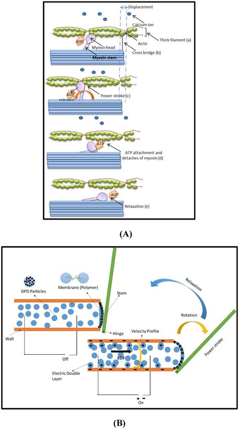
                                            Objective. With an overview of the natural mechanism of muscle contraction in nature, almost all living
                                            things use a common mechanism for muscle contraction and movement. The contraction mechanism of a real
                                            muscle and the present proposal are shown in Fig. 1A. Initially, by stimulating the nervous system, the electrical
                                            signal causes the release of calcium ions from sarcoplasmic reticulum and calcium ions cause ATP change to
                                            ADP in myosin and the movement of the myosin stem (a). The result of stem movement is the binding to actin,
                                            which is called cross bridge (b) and the action of muscle contraction (c). In the opposite direction, with the
                                            arrival of an electrical signal to end the contraction process, all the calcium ions are collected in sarcoplasmic
                                            reticulum and ATP will connect to the myosin (d), it causes the myosin to move in the opposite direction and
                                            the muscle will be relaxed (e)1–3.
                                                In the present proposal in Fig. 1B, the electro-osmotic method is used to move the fluid like the transfer
                                            of ions in normal muscle (see a). Electro-osmotic is a form of pumping fluid by electric force. The fluid moves
                                            under the influence of electro-osmotic flow and causes to stretch the membrane or polymer chain when fluid
                                            flow pushes it (see b). The tension of the polymer causes the transfer of power to the hinged stem from one side
                                            and the stem will move angularly (see c). When the electric flow cut off, the electro-osmotic force is zero and the
                                            fluid moves backwards (see d) and the artificial myosin stem is relaxed (see e). Such a movement is the beginning
                                            of a muscle contraction like a real muscle. To simulate this artificial muscle contraction, the three basic topics of
                                            electro-osmotic flow, DPD method, and polymer or membrane chain are briefly reviewed in the Sect. 2.
                                                In this paper, according to the natural movement of myosin to contract a muscle, proposed method employs
                                            DPD method to simulate EOF and performance of membrane which transmute the fluid pressure to displace-
                                            ment of an artificial myosin as a heart of an artificial muscle. Factors affecting the occurrence of this movement
                                            have been investigated in two general categories of factors affecting the electro-osmotic flow and factors affecting
                                            the DPD method and membrane.

                                            Methodology
                                            In order to simulate the mentioned model, it is necessary to check the equations of three sections including
                                            electro-osmotic flow, polymer chain, DPD simulation method, which is presented in the following.

                                            Electro‑osmotic flow (EOF).            Normally, without applying electrical field (E0) to a micro-channel, the fluid
                                            is electrolytically neutral, but when an electric field is established, the fluid in the channel begins to move as it
                                            exits the electrolytic neutral state. This type of movement and pumping of fluid is called electro-osmotic flow
                                            (EOF). The root of this motion is in the electric double layer (= 1/k). In other words, because the surface is

          Scientific Reports |   (2021) 11:2235 |                https://doi.org/10.1038/s41598-021-81608-7                                                      2

Vol:.(1234567890)
www.nature.com/scientificreports/

                                  Figure 1.  A thin filament of natural muscle mechanism and proposed artificial mechanism. Natural muscle
                                  (filament) movement (A): action potential (a), bridge connection (b) and power transfer operation (c),
                                  separation (d) and relaxation (e)34. Artificial muscle movement (B): EOF/on and transfer of power to the
                                  membrane, stem and angular rotation, also EOF/off and relaxation.

Scientific Reports |   (2021) 11:2235 |              https://doi.org/10.1038/s41598-021-81608-7                                              3

                                                                                                                                        Vol.:(0123456789)
www.nature.com/scientificreports/

                                            charged and the electrolyte solution has positive and negative ions and they are affected by the wall, ions of the
                                            opposite types should be absorbed by the wall, while ions of the same kind should be disposed of each other.
                                            This particular arrangement is often referred to as the electric double layer. Inside this layer and adjacent to
                                            the wall, a very thin layer (around a nanometer) is situated which is called stern layer. The ions of this layer are
                                            completely attached to the wall and are immobile. As the next layer is mobile layer with a thin thickness around
                                            a few nanometers to a few micrometers widths, called the diffuse layer, thus there is a shear layer between them
                                            and flow movement will start from this layer. In the diffuse layer, the concentration of ions opposite the wall
                                            decreases to be equal to the concentration of ions in the w ­ all20.
                                                One of the basic parameters in the arrangement of ions is the electrical potential at the surface or the poten-
                                            tial at the interface between the stern layer and the zeta scattering layer is the zeta potential (ψ0) and its value
                                            depends on the solid and fluid surface of the electrolyte. The fluid on the one hand is affected by the zeta potential
                                            and on the other hand fluid is under effect of electric field which consequently will cause the fluid to move. The
                                            smaller the thickness of the double layer is resulted from higher ionic concentration of solvent and it will affect
                                            on the velocity profile or gives higher the dimensional ratio of kH parameter (channel height × inversed electric
                                            double layer thickness).
                                                The equation that governs this type of motion is Poisson equation which is
                                                                                                              ρe
                                                                                                ∇2� = −                                                       (1)
                                                                                                              ǫ
                                            where ψ is the electric potential, ρe is net charge density and ǫ is relative permittivity of the solvent. ψ depends
                                            on geometry and boundary conditions and net charge density can be extracted from Eq. (1). Considering the
                                            electric field of E0 and substituting in Eq. (2), EOF force can be calculated:
                                                                                                  F e = E0 ρe                                                 (2)
                                               This force is applied to all fluid particles and causes the motion and transmission of the momentum. The
                                            result of this force is the transfer of force to the membrane and the swelling of membrane, which is explained in
                                            the next section on how to simulate DPD particles and membrane ­simulation25.

                                            Polymer membrane (polymer chain).              The main innovation of this research is in the swelling of mem-
                                            brane and transfer of fluid power to move the artificial myosin. To simulate this thin membrane, it is sufficient to
                                            place an impermeable polymer chain in two dimensions across the channel that can hold particles and transmit
                                            power. For modeling of a polymer chain, it is sufficient to consider a number of beads and springs attached to
                                            them and consequently spring force should be added in conservative force. This force is:
                                                                                                   p
                                                                                                 Fij = Shb rij                                                (3)

                                            where the spring hardness coefficient is Shb or the harmonic bond constant. Two important indicators in the
                                            displacement of a polymer chain are considered including the radius of gyration and the velocity auto-correla-
                                            tion function (VACF). The radius of gyration indicator can describe the distribution the dimensions of a poly-
                                            mer chain. The radius of gyration is the root mean square distance ( RG
                                                                                                                  2 ) of particle from the center of mass (cm)
                                            which is presented a­ s31–33,37,38
                                                                                         n
                                                                                  2   1                       1  2
                                                                                 RG =      (ri − rmean )2 = 2        r                                  (4)
                                                                                     n
                                                                                         1
                                                                                                             2n ij ij
                                                                                                               →          
                                            in which, rmean is the mean position of the polymer chain, rij = − r i −−→r j  and n is the beads number in a
                                            monomer. Also, for calculation of VACF, at the first, velocity of the center-of-mass of the polymer chain (vi )
                                            should be calculated:
                                                                                                           n vi (i)
                                                                                          vi (itvacf ) =                                                      (5)
                                                                                                            i=1 n

                                            where itvacf is iteration number of time step and consequently it will use for updating and label of the register.
                                            Then, considering number of time step, the VACF should be updated:
                                                                                                it
                                                                                   Vvacf (it) =     vi (it t0 )vi (itt+t0 )                               (6)
                                                                                                       i=1

                                            where (it t0 ) and (itt+t0 ) are the origin time of polymer and summation of origin time with delay time. It should be
                                            noticed that polymer chain is not influenced from EOF and motion of polymer chain is resulted from momentum
                                            transfer of fluid particles which the fluid motion is caused from ­EOF39.

                                            Dissipative particle dynamics (DPD). According to this method, a number of molecules are considered
                                            in a cluster and due to the large grain size of the simulation method, the run time of simulation is so faster and
                                            the simulation would be carried out in a larger scale than the molecular simulation method and in a smaller scale
                                            than the continuous CFD method. The formulation of this method is based on Newton’s method in which states
                                            the temporal evolution of each DPD particle   →as a set of molecules/atoms is associated to the velocity of the DPD
                                                                                          −
                                            particles (−
                                                       →v i ) and consequently the force ( F i ) applied to each of the particles can be calculated:

          Scientific Reports |   (2021) 11:2235 |                https://doi.org/10.1038/s41598-021-81608-7                                                     4

Vol:.(1234567890)
www.nature.com/scientificreports/

                                                                                               −
                                                                                               →   d−
                                                                                                    →ri
                                                                                               vi=                                                             (7)
                                                                                                    dt

                                                                                                  d−
                                                                                                   →vi   −
                                                                                                         →
                                                                                             mi        = Fi                                                    (8)
                                                                                                   dt
                                                                                                                                 −
                                                                                                                                 →
                                  where −
                                        →r i is position of particle with mass of m−i ). Generally, total inter-particle force ( F i ) consists of two main
                                                                                    →
                                  components including external or EOF force ( F EOF ) in this research and internal forces including FijC or the
                                  conservative force, FijD or the dissipative force and FijR or the random force.
                                                             −
                                                             →       −
                                                                     →           −
                                                                                 →            −
                                                                                              →            
                                                              F i = F external + F internal = F EOF +         [FCij + FD     R
                                                                                                                       ij + Fij ]                       (9)
                                                                                                                         j�=i

                                                                                                        
                                                                                                    rij
                                                                                          aij 1 −             r̂ij , rij < rc     p
                                                                           FCij   =                 rc                         + Fij                          (10)
                                                                                          0,                          rij ≥ rc

                                                                                  FD        D
                                                                                   ij = −γ ω (rij )(
                                                                                                    rij · vij )(rij )                                        (11)

                                                                                           FRij = σ ωR (rij )θijrij                                          (12)
                                  where aij is the repulsive parameter between particle i and j which can be extended to interaction between fluids,
                                  walls and polymers particles, rc is the cut-off radius normalized to unity, rij = (ri—rj), rij =|rij|, and rij = rij /rij . Also
                                  γ and σ are the constant coefficients, vij = (vi—vj), ωD and ωR are weight functions:
                                                                                               
                                                                            R  2                   r
                                                                       D                             1 − rijc , rij < rc
                                                                     ω rij = ω rij           =                                                                 (13)
                                                                                                  0,            rij ≥ r

                                  θij in the random force is a random function due to meso-scale simulation which has zero mean and unit vari-
                                  ance properties. Velocity-Verlet (DPD-VV) algorithm is an applied method to solve equations and update the
                                  position and velocity of particles. Also, according to Duong-Hong et al.25,37, double layer of frozen particles at the
                                  wall with consideration of radius of cut off (rc ) and the bounce-back condition are used as a boundary condition
                                  implementation on walls.

                                  Results and discussion
                                  In order to evaluate the obtained results, first, the results are evaluated and validated in a simple channel under
                                  the influence of electro-osmotic flow, and then the proposed artificial muscle will be simulated in different
                                  conditions.

                                  Validation. As mentioned in the numerical method section, the electro-osmotic force is formed by imple-
                                  menting the electric field in the fluid, considering the effect of electric charge density and electric field (see
                                  Eq. 2), the EOF force in the fluid particles is formed in a double electric layer that starts moving from the walls
                                  border and finally the velocity profile is shaped. The final velocity profile is a function of parameters such as
                                  ionic concentration (i ∝ k) parameter, zeta potential effect due to wall material and E0 or applied electric field.
                                      One of the basic parameters in electro-osmotic flow is the ionic concentration of the fluid. Without ionic
                                  property, an electric double layer is not formed and having a minimum value of ionic property is necessary for
                                  fluid transfer. According to the Eq. 1 ionic concentration has an inverse relationship with the Debye length, in
                                  other words, higher the ionic concentration provides the shorter Debye length and the flatter the velocity profile
                                  and vice versa. Dimensionless kH parameter describes the ratio of channel width to Debye length. By increasing
                                  the kH parameter, amount of flow velocity is increased to a certain extent and saturation is formed, and after a
                                  certain limit, the velocity profile just becomes flatter.
                                      Figure 2A shows the velocity profile diagram for different values of kH parameters based on the Table 1.
                                  As shown, the DPD method is in proper agreement with the analytical results in the simple channel. Also, as
                                  the amount of ionic concentration of the fluid increases, the velocity profile becomes flatter and also the veloc-
                                  ity value increases to a certain extent, which there is no change in the maximum value but the velocity profile
                                  becomes flatter. In the same way in mentioned figure, the average of velocity profiles calculated by DPD method
                                  has been compared with analytical results in a wide range of changes in channel height, k parameters (Fig. 2B),
                                  electric field, ψ0 (Fig. 2C). The accuracy of all results is reported with an error of less than 10%. As can be seen,
                                  changes in ψ0 and electric field have a linear relationship with increasing velocity, but the ion concentration
                                  non-linearly increases to a certain velocity and no significant change is seen after a certain amount. Also, the
                                  validation of polymer chain in nano channel has been reported in ­ref31. It can be concluded that on a particle
                                  scale, the DPD method has a proper accuracy in analyzing the complex test cases such as electro-osmotic flow
                                  and can be simulated for more complex situations such as simulation of a micro myosin performance in EOF.

Scientific Reports |   (2021) 11:2235 |                  https://doi.org/10.1038/s41598-021-81608-7                                                              5

                                                                                                                                                           Vol.:(0123456789)
www.nature.com/scientificreports/

                                                                                                                                                   DPD (kH = 25)
                                                                                                                                                   DPD (kH = 16)
                                                                                    15                                                             DPD (kH = 8)
                                                                                                                                                   DPD (kH=5)
                                                                                                                                                   DPD (kH=1.6)
                                                                                                                                                   Analytical
                                                                                    10

                                                                                    5

                                                                            Y(nm)
                                                                                    0

                                                                                    -5

                                                                                  -10

                                                                                       -1      0     1              2         3       4           5           6
                                                                                                                    V (µm/s)

                                                                                                                        (A)

                                      800                                                                                               250                                                                           50
                                                                                                   0.3
                                                                                                                                                                                                                      45

                                                                                                                                        200
                                      600
                                                                    DPD (H, k=0.032)               0.25                                                                                                               40
                                                                    DPD (k, H=50 nm)

                                                                                                                                                                                                                           Zeta P. (mV)
                                                                    Analytical (H, k=0.032)
                                                                    Analytical (k, H=50 nm)                                                                                                                           35
                                                                                                   0.2                                  150
                                                                                                                                  E0 (V/m)
                                                                                                         k (1/nm)
                                 H (nm)

                                                                                                                                                                                                                      30
                                      400
                                                                                                   0.15
                                                                                                                                        100                                                                           25

                                                                                                   0.1                                                                                                                20
                                      200                                                                                                                                DPD (E0 (Y1), zeta = -25 mV, kH=16)
                                                                                                                                             50                          DPD (zeta (Y2), E0 = 50 V/m, kH=16)
                                                                                                                                                                         Analytical (E0 (Y1), zeta = -25 mV, kH=16)   15
                                                                                                   0.05                                                                  Analytical (zeta (Y2), E0 = 50 V/m, kH=16)

                                                                                                                                                                                                                      10
                                               2     4         6     8       10          12   14                                                  0.5     1        1.5        2        2.5        3        3.5
                                                           Average Velocity (µm/s)                                                                            Average Velocity (µm/s)

                                                                    (B)                                                                                           (C)
                                                     Figure 2.  Validation of EOF-DPD results using analytical results. Comparison of DPD method and analytical
                                                     solution: velocity profiles in different kH parameters (A) for E0 = 250 V/m, zeta potential − 25 mV and average
                                                     velocity influenced from different reverse of EDL (k) and channel height, E0 = 250 V/m, ψ0=− 25 mV (B) and
                                                     different electric fields and zeta potentials, kH = 16 (C).

                                                      DPD-Parameters                 Values
                                                      aij25                          75
                                                      awij25                         8.66
                                                      Channel length                 20 × 20 nm
                                                      Particles density              10
                                                      Numbers of particles           4000
                                                      σ                              3
                                                      rc                             1
                                                      Polymer-Parameters             Values
                                                      Numbers of beads               50
                                                      dt                             0.001
                                                      S                              8000

                                                     Table 1.  DPD and polymer constant parameters.

          Scientific Reports |            (2021) 11:2235 |                          https://doi.org/10.1038/s41598-021-81608-7                                                                                                            6

Vol:.(1234567890)
www.nature.com/scientificreports/

                                  Displacement of polymer artificial myosin through electro‑osmotic nano flow.                     Fluid transfer
                                  is always accompanied by momentum transfer, and if this fluid force is transferred properly, it will be able to
                                  move objects. In one classification, changes in polymer motion can be divided into three categories: parameters
                                  affected by electro-osmotic flow and parameters affected by fluid and membrane which they are investigated in
                                  the following.

                                  Impact of EOF parameters. The electro-osmotic force causes the fluid to move and the fluid enters its force into
                                  the membrane and will cause the membrane to swell. Membrane swelling also increases the ability of the stem
                                  to move. Placing a polymer membrane at the end of the channel will prevent particles from moving out and the
                                  swelling of the membrane will be simulated. Also, by transferring force from the membrane to the stem, it causes
                                  the stem to rotate. All the conditions used in the simulation are given in Table 1. The results of this simulation
                                  over time are shown in Fig. 3 in various motion forms. As can be seen, with the movement of the fluid by the
                                  electro-osmotic force and the momentum transfer of the fluid, swelling is created in the membrane and finally
                                  the movement of the polymer and the stem is resulted (Fig. 3A). In practice, this method can be used to create
                                  motion with significant displacement, and finally the motion of the solid object displacement can be obtained
                                  which angular displacement of stem over iteration numbers is depicted in Fig. 3B.

                                  Effect of kH parameter. Changes in ionic concentration or Debye length (kH parameter) also affects the rate of
                                  membrane inflation and will cause different displacements. Figure 4A shows the displacement of the membrane
                                  for different kH values. As it is clear, with increasing kH parameter, no significant changes in displacements
                                  are observed, and this is a sign of reaching the ionic concentration to saturation condition. Also, the radius of
                                  rotation of the polymer or membrane chain has not changed significantly (Fig. 4B) because the displacement
                                  rate is not conspicuous. Also, the VACF has not changed so much because there are no significant velocity and
                                  dynamics changes (Fig. 4C). It can be concluded that by increasing the ionic concentration of the membrane to
                                  a certain extent less than 8% increase in displacement can be achieved and it has a small variation amount in the
                                  radius of rotation and VACF.

                                  Effect of zeta potential and electric field. The two electro-osmotic parameters that will have a major impact
                                  on the displacement of the velocity profile as well as the polymer chain are the effect of the electric field and the
                                  zeta potential. The first parameter can be increased or decreased during movement and is important from the
                                  control point of view, while the second parameter is related to the material of wall and affects the strength of
                                  the electro-osmotic flow during the construction phase. The changes of these parameters are almost linear on
                                  the velocity profile and due to the effect of membrane elasticity; no parameter will have an exact linear effect on
                                  polymer membrane. The Fig. 5A shows the effect of zeta potential on the displacement of the membrane. As can
                                  be seen, by increasing the zeta potential to ten times, an increasing of about 40% in displacement is obtained, and
                                  a significant effect is observed on the radius of gyration and the VACF (Fig. 5B,C). If such a study is carried out
                                  on changes in the electric field, we will reach similar results. In Fig. 6A by enhancing the electric field to 5 times, a
                                  23% of increasing in displacement is gained, and a significant effect has been seen on other properties such as the
                                  radius of gyration and the VACF (Fig. 6B,C). Note that excessive increase of the field has an electrolysis effect and
                                  is one of the limiting parameters in the amount. According to the ­references22–25, the safe ranges were chosen in
                                  this paper. It can be concluded that the effect of zeta potential and electric field have a great effect on the displace-
                                  ment of the membrane and in the manufacturing phase the use of high potential zeta materials is appropriate
                                  and in the control of membrane displacement, the use of variable electric field is a significant variable.
                                      It is obvious that by studying the ratio of the average velocity of the polymer membrane within 8.5 s and also
                                  the average ratio of strain on the elastic membrane in Table 2, it can be concluded that the performance (higher
                                  velocity and elongation) for kH more than 8 would be higher than other cases. Also, higher polymer chain per-
                                  formance is related to higher zeta potential and electric field.

                                  Impact of DPD fluid and polymer parameters. As it is obvious (see Eqs. 3–12), in addition to the parameters that
                                  are affected by the electro-osmotic flow, there are other parameters which they depend on type of fluid, the col-
                                  lision of the fluid with the polymer chain or polymer to polymer. These parameters in this research are divided
                                  into four general categories: repulsive parameter or parameter of collision of fluid with polymer and collision of
                                  polymer particles with each other, polymer chain length parameter, number of beads used in membrane simula-
                                  tion, particles density or determination of number of particles and stiffness parameter between beads.
                                      In Fig. 7, the effect of the parameters can be understood by comparing Fig. 3, considering kH = 8, E0 = 250 V/m
                                  and Ψ0 = − 25. Respectively, from left to right by changing the chain length parameter from 50 to 30 (Fig. 7A),
                                  almost 30% reduction in displacement, by changing the repulsive parameter between polymer-DPD particles
                                  and polymer–polymer particles (see Eq. 10) 4 times (a = 4) around 22% drop in displacement (Fig. 7B), by chang-
                                  ing the coefficient of spring stiffness (harmony hardness coefficient) between the beads 0.5 times, about 36%
                                  enhancement in displacement (Fig. 7C) and by decreasing the particle density from 10 to 5, about 19% reduction
                                  in displacement are observed (Fig. 7D). Obviously, by reducing the number of beads, the intermediate springs
                                  between beads are stretched more and the membrane stiffness will be higher and there is less displacement, or
                                  by decreasing the stiffness coefficient of the springs, an increase in the length of the springs (strain) will be seen.
                                  Also, the changing of the membrane material and type of DPD fluid, using the manipulation of the repulsive
                                  factor, the displacement of the membrane is affected and by increasing the repulsion coefficient, less displacement
                                  is resulted which these parameters are reviewed and analyzed further in next sections.

Scientific Reports |   (2021) 11:2235 |                 https://doi.org/10.1038/s41598-021-81608-7                                                       7

                                                                                                                                                    Vol.:(0123456789)
www.nature.com/scientificreports/

                                                40                                                                              40                                                                 40

                                                35

                                                30                                                                                                                                                 30

                                                25

                                                20                                                                              20                                                                 20

                                       Y (nm)

                                                                                                                       Y (nm)

                                                                                                                                                                                          Y (nm)
                                                15
                                                      t=1.5 s                                                                         t = 1.7                                                           t=2s
                                                10                                                                                                                                                 10

                                                5

                                                0                                                                               0                                                                  0

                                                -5

                                            -10                                                                                                                                                -10
                                               -4           -2    0   2    4       6                       8    10               -4         -2      0      2    4       6      8   10                               0            5   10
                                                                      X (nm)                                                                               X (nm)                                                       X (nm)

                                                40                                                                              40                                                                 40

                                                30                                                                              30                                                                 30

                                                20                                                                              20                                                                 20
                                       Y (nm)

                                                                                                                       Y (nm)

                                                                                                                                                                                          Y (nm)
                                                      t = 3.5 s                                                                       t = 4.5 s                                                         t = 5.5 s
                                                10                                                                              10                                                                 10

                                                0                                                                               0                                                                  0

                                            -10                                                                             -10                                                                -10
                                                                  0            5                                10                                  0               5              10                               0            5   10
                                                                      X (nm)                                                                               X (nm)                                                       X (nm)

                                                40                                                                              40                                                                 40

                                                                                                                                                                                                   35

                                                30                                                                              30                                                                 30

                                                                                                                                                                                                   25

                                                20                                                                              20                                                                 20
                                       Y (nm)

                                                                                                                       Y (nm)

                                                                                                                                                                                          Y (nm)
                                                                                                                                                                                                   15
                                                                                                                                      t = 7.5 s                                                         t = 8.5 s
                                                       t = 6.5
                                                10                                                                              10                                                                 10

                                                                                                                                                                                                   5

                                                0                                                                               0                                                                  0

                                                                                                                                                                                                   -5

                                            -10                                                                             -10                                                                -10
                                                                  0            5                                10                                  0               5              10                               0            5   10
                                                                      X (nm)                                                                               X (nm)                                                       X (nm)

                                                                                                                                                         (A)

                                                                                                           80
                                                                                       Rotation (degree)

                                                                                                           60

                                                                                                           40

                                                                                                           20

                                                                                                                2000    3000               4000         5000   6000         7000   8000
                                                                                                                                                Iteration number

                                                                                                                                                        (B)

                                                     Figure 3.  Rotation of stem over time. Displacement of membrane and step due to EOF, kH = 8, E0 = 250 V/m,
                                                     ψ0= − 25 mV (A). Angular displacement of stem over iteration numbers (B).

          Scientific Reports |   (2021) 11:2235 |                                  https://doi.org/10.1038/s41598-021-81608-7                                                                                                             8

Vol:.(1234567890)
www.nature.com/scientificreports/

                                                                           5
                                                                                          kH = 0.02
                                                                                          kH = 0.2
                                                                                          kH = 2

                                                                  Y (nm)
                                                                                          kH = 8
                                                                           0              kH = 13

                                                                           -5

                                                                                4   4.5          5            5.5                                                     6     6.5
                                                                                              Displacement (nm)

                                                                                                        (A)

                              40

                                                                                                               Velocity autocorrelation function ( µ m/s)2
                                                                                                                                                             1
                              35                                                                                                                                                            kH   = 0.02
                                                                                                                                                                                            kH   = 0.2
                                                                                                                                                             0                              kH   =2
                              30                                                                                                                                                            kH   =8
                                                                                                                                                                                            kH   = 13
                  RG 2 (nm)

                              25                                                                                                                             -1
                                                  kH = 0.02
                                                  kH   =   0.2
                              20                  kH   =   2
                                                  kH   =   8                                                                                                 -2
                                                  kH   =   13
                              15

                                                                                                                                                             -3
                              10

                                   0     0.2               0.4             0.6      0.8             1                                                             0       0.2        0.4          0.6     0.8    1
                                                  Dimensionless time                                                                                                              Dimensionless time

                                                            (B)                                                                                                                       (C)
                                          Figure 4.  Changes of kH parameter on EOF with E0 = 250 V/m and Ψ0 = − 25 mV and impermeable polymer
                                          membrane displacement. Different displacement of polymer membrane by changing kH parameter (A).
                                          Variation of radius of gyration and VACF over dimensionless time (t/tmax) by changing the kH parameter (B,C).

                                          Impact of polymer beads number. Since a number of beads and springs are used in the simulation of a polymer
                                          membrane, a change in their number will affect the elasticity of the membrane. By reducing the number of beads
                                          and considering the beginning and end of the beads are determined and constant, it is clear that the membrane
                                          for installation across the channel in the transverse direction should be stretched more and its displacement in
                                          the longitudinal direction is reduced. In Fig. 8A change in membrane displacement is clearly observed, and also
                                          with a decrease in displacement, a decrease in the gyration radius, and a velocity correlation function (VACF)
                                          has been resulted due to less movement (Fig. 8B,C). According to the VACF, it can be detected that a strong
                                          nonlinear relationship prevails in the number of fewer beads than the number of more beads. Such a result is
                                          also observed in the displacement of the polymer chain in such a way that by increasing the beads from 20 to
                                          30, the displacement changes by about 9% (highly nonlinear trend) and in increasing the beads from 30 to 40 or
                                          from 40 to 50, the displacement changes proportional and more which these variations are reported about 20%
                                          (low nonlinear behavior).

                                          Impact of DPD‑repulsive parameter. The most important parameter for determining the material of the fluid
                                          or polymer is the repulsive factor, which is derived from the coefficients of the Leonard Jones equation. In this
                                          research, the collision of fluid with polymer and also the collision of polymer with polymer have been investi-

Scientific Reports |           (2021) 11:2235 |                            https://doi.org/10.1038/s41598-021-81608-7                                                                                                9

                                                                                                                                                                                                                Vol.:(0123456789)
www.nature.com/scientificreports/

                                                                              5

                                                                                                 Zeta = -25 mV
                                                                                                 Zeta = -100 mV

                                                                     Y (nm)
                                                                                                 Zeta = -250 mV
                                                                              0

                                                                              -5

                                                                                   4   4.5   5      5.5    6       6.5   7                                             7.5       8   8.5     9
                                                                                             Displacement (Dimensionless)

                                                                                                                   (A)

                                                                                                                                                                        3

                                                                                                                         Velocity autocorrelation function ( µ m/s)2
                                        40                                                                                                                             2.5
                                                                                                                                                                        2                            Zeta -25 mV
                                                                                                                                                                                                     Zeta -100 mV
                                        35                                                                                                                             1.5                           Zeta -250 mV

                                                                                                                                                                        1
                                        30
                                                                                                                                                                       0.5
                            RG 2 (nm)

                                                                                                                                                                        0
                                        25                    Zeta = -25 mV
                                                              Zeta = -100 mV                                                                                -0.5
                                                              Zeta = -250 mV
                                        20                                                                                                                              -1
                                                                                                                                                            -1.5
                                        15
                                                                                                                                                                        -2
                                                                                                                                                            -2.5
                                        10
                                                                                                                                                                        -3
                                                                                                                                                            -3.5
                                             0     0.2         0.4             0.6           0.8               1                                                             0         0.2          0.4            0.6   0.8   1
                                                            Dimensionless time                                                                                                                   Dimensionless time

                                                                 (B)                                                                                                                                 (C)
                                                    Figure 5.  Changes of zeta potential on EOF and polymer membrane. Different displacement of polymer
                                                    membrane by changing the zeta potential, kH = 8, E0 = 250 V/m (A). Variation of radius of gyration and VACF
                                                    over dimensionless time (t/tmax) by changing the zeta potential (B,C).

                                                    gated using multiplying the repulsive parameter of Table 1 by constant parameter (a). The change of this param-
                                                    eter on polymer displacement is given in the Fig. 9A. As it is known, by changing this parameter (a = 2, 4 (fluid-
                                                    polymer and polymer–polymer collision)) the maximum variation has decreased by about 16%. As expected,
                                                    changes in radius of gyration and VACF change slightly (Fig. 9B,C). It can be concluded that depending on the
                                                    type of fluid used, by changing this parameter, a suitable material of the polymer can be obtained, but the elastic
                                                    property of the polymer must also be considered, which is examined in the next section.

                                                    Impact of harmonic bonding parameter. The coefficient of elasticity between the beads determines the elastic-
                                                    ity of the membrane. Whatever mentioned coefficient is increased, the harder the elongation of the spring and
                                                    the less displacement will be eventually formed. In the Fig. 10A, for different values of this bond coefficient,
                                                    which is called by different titles such as harmonic bond coefficient, spring coefficient or elasticity coefficient,
                                                    is presented. As can be seen, by increasing this coefficient, less displacement is achieved because the resistance
                                                    force of the membrane against fluid movement would be higher. Considering the changing this parameter as
                                                    shown in Fig. 10B,C, conspicuous dynamics motion is reported by in investigation of radius of gyration and
                                                    VACF. In practice, this coefficient has a certain limit and by passing this limit, a notch is formed in the mem-
                                                    brane. It can be concluded that this parameter is the most important parameter in determining the amount of

          Scientific Reports |           (2021) 11:2235 |                          https://doi.org/10.1038/s41598-021-81608-7                                                                                                      10

Vol:.(1234567890)
www.nature.com/scientificreports/

                                                                    5

                                                                                          E0 = 50 V/m
                                                                                          E0 = 100 V/m

                                                           Y (nm)
                                                                                          E0 = 250 V/m
                                                                    0

                                                                    -5

                                                                         4    4.5         5      5.5       6                                          6.5              7    7.5
                                                                                              Displacement (nm)

                                                                                                         (A)

                                                                                                                                                              2
                         40
                                                                                                               Velocity autocorrelation function ( µ m/s)2   1.5
                                                                                                                                                                                       E0 = 50 V/m
                         35                                                                                                                                   1                        E0 = 100 V/m
                                                                                                                                                                                       E0 = 250 V/m
                                                                                                                                                             0.5
                         30
                                                                                                                                                              0
             RG 2 (nm)

                         25                                                                                                                       -0.5

                                               E0 = 50 V/m                                                                                                    -1
                         20                    E0 = 100 V/m
                                               E0 = 250 V/m                                                                                       -1.5

                         15                                                                                                                                   -2

                                                                                                                                                  -2.5
                         10
                                                                                                                                                              -3

                                                                                                                                                  -3.5
                              0         0.2          0.4             0.6            0.8            1                                                               0       0.2       0.4        0.6    0.8   1
                                                Dimensionless time                                                                                                                Dimensionless time

                                                      (B)                                                                                                                             (C)
                                              Figure 6.  Changes of electric field on EOF and polymer membrane. Different displacement of polymer
                                              membrane by changing the electric field, kH = 8, Ψ0 = − 25 mV (A). Variation of radius of gyration and VACF
                                              over dimensionless time (t/tmax) by changing the electric field (B,C).

                                              elasticity of a membrane and by decreasing the elasticity coefficient to 0.5 times, 36% increase in displacement
                                              would be obtained.

                                              Impact of density parameter. Since we are dealing with particles and the fluid is not continuum, the particles
                                              density parameter (PD) which is related to the number of particles (NP), NP = PD × DL × DY in a simulation box
                                              (DL × DY) is very effective in the efficiency of stem movement. In this study, unlike the previous cases where this
                                              parameter was 10, in these cases, considering the Fig. 3 conditions, this parameter has been reduced to 3, 5 and
                                              7, and the results of these changes are shown in Fig. 11. Initially, in Fig. 11A, as can be seen, with decreasing the
                                              number of particles, the ability to move in a certain period of time decreases and the stem has unstable behavior
                                              in the state of PD = 3. By increasing the PD to 5, a slight improvement in displacement has been observed and in
                                              PD = 7, it has shown better performance. It can be concluded that with the increasing of density of particle, more
                                              momentum of particles will transfer to the polymer membrane. In Fig. 11B displacement of the polymer chain
                                              is presented without showing the fluid particles which has achieved more displacement in PD = 7 at t = 8.5 s and
                                              compared to the Fig. 3 (PD = 10), PD = 7 has been observed almost 21% less displacement. Also, the study of the
                                              parameters of gyration radius and VACF show that less perturbation in chain motion is observed with increasing
                                              density or higher PD parameter.

Scientific Reports |              (2021) 11:2235 |                           https://doi.org/10.1038/s41598-021-81608-7                                                                                              11

                                                                                                                                                                                                                 Vol.:(0123456789)
www.nature.com/scientificreports/

                                                         Parameter Vi
                                                                   Vj                                         Parameter ǫǫij
                                                         i, j = 1–5 (kH = 0.02. 0.2, 2, 8, 13)                i, j = 1–5 (kH = 0.02. 0.2, 2, 8, 13)
                                                                                                                 
                                                         V5/V1 = 1.28                                         ǫ5 ǫ1 = 1.26
                                                                                                                 
                                                         V5/V2 = 1.22                                         ǫ5 ǫ2 = 1.23
                                                                                                                 
                                                         V5/V3 = 1.14                                         ǫ5 ǫ3 = 1.17
                                                                                                                 
                                                         V5/V4 = 1.04                                         ǫ5 ǫ4 = 1.04
                                                         Parameter Vi Vj                                      Parameter ǫǫij
                                                         i, j = 1–3 (zeta = − 25, − 100, − 250)               i, j = 1–3 (zeta = − 25, − 100, − 250)
                                                                                                                 
                                                         V3/V1 = 1.45                                         ǫ3 ǫ1=1.33
                                                                                                                 
                                                         V3/V2 = 1.28                                         ǫ3 ǫ2 = 1.23
                                                         Parameter Vi
                                                                   Vj                                         Parameter ǫǫij
                                                         i, j = 1–3 ( E0 = 50, 100, 250)                      i, j = 1–3 ( E0 = 50, 100, 250)
                                                                                                                 
                                                         V3/V1 = 1.95                                         ǫ5 ǫ1=1.65
                                                                                                                 
                                                         V3/V2 = 1.45                                         ǫ5 ǫ2 = 1.37

                                                         Table 2.  Ratio of average velocity and strain of polymer chain for different kH, zeta potential and electric field
                                                         parameter.

                                    40                                                                       40                                                               40

                                                                                                                                                                              35

                                    30                                                                       30                                                               30

                                                                                                                                                                              25

                                    20                                                                       20                                                               20
                           Y (nm)

                                                                                                    Y (nm)

                                                                                                                                                                     Y (nm)
                                                                                                                                                                              15
                                         t = 8.5 s                                                                 t = 8.5 s                                                       t = 8.5 s
                                    10                                                                       10                                                               10

                                                                                                                                                                              5

                                    0                                                                        0                                                                0

                                                                                                                                                                              -5

                                 -10                                                                      -10                                                             -10
                                    -4         -2    0     2     4      6      8     10                                            0                   5        10                             0             5   10
                                                           X (nm)                                                                         X (nm)                                                    X (nm)

                                                         (A)                                                                           (B)                                                         (C)
                                                                                                    40

                                                                                                    35

                                                                                                    30

                                                                                                    25

                                                                                                    20
                                                                                           Y (nm)

                                                                                                    15
                                                                                                              t = 8.5 s
                                                                                                    10

                                                                                                      5

                                                                                                      0

                                                                                                     -5

                                                                                                -10
                                                                                                   -5                          0                   5       10
                                                                                                                                       X (nm)

                                                                                                                                       (D)
                                                         Figure 7.  Effect of DPD-polymer parameters on angular rotation of stem compared to Fig. 3 (last frame).
                                                         Variations of beads number (left to right respectively) from 50 to 30 (A), repulsive parameters 4 times (B),
                                                         harmony hardness coefficient 0.5 times (C) and particle density 0.5 times (D).

                                                             As can easily be resulted in Table 3, by increasing the number of beads, the ratio of velocity and strain (per-
                                                         formance) has increased but stronger repulsive parameter has negative effect on performance from velocity and
                                                         stain ratio aspect. Also, stronger bonding coefficient provides lower ratios (stiff materials) while higher density
                                                         not only gives higher displacement but also displacement of stem is more stable.

          Scientific Reports |           (2021) 11:2235 |                           https://doi.org/10.1038/s41598-021-81608-7                                                                                   12

Vol:.(1234567890)
www.nature.com/scientificreports/

                                                                    5

                                                                                                                                                               L = 20
                                                                                                                                                               L = 30

                                                           Y (nm)
                                                                                                                                                               L = 40
                                                                    0
                                                                                                                                                               L = 50

                                                                    -5

                                                                         4   4.5   5     5.5   6   6.5       7                                        7.5      8   8.5    9
                                                                                           Displacement (nm)

                                                                                                   (A)

                         40                                                                                                                           2                                L = 20

                                                                                                         Velocity autocorrelation function (µ m/s)2                                    L = 30
                                                                                                                                                                                       L = 40
                         35                                                                                                                                                            L = 50
                                                                                                                                                      1

                         30
                                                                                                                                                      0
             RG 2 (nm)

                         25                     L = 20
                                                L = 30
                                                L = 40                                                                                                -1
                         20                     L = 50

                         15                                                                                                                           -2

                         10
                                                                                                                                                      -3

                         5
                              0         0.2          0.4             0.6           0.8         1                                                           0        0.2          0.4            0.6   0.8   1
                                                Dimensionless time                                                                                                            Dimensionless time

                                                         (B)                                                                                                                      (C)
                                              Figure 8.  Effect of number of beads on membrane. Displacement of polymer chain in EOF for different beads
                                              number (A). Changes of radius of gyration and VACF over dimensionless time (t/tmax) considering different
                                              beads number (B,C).

                                              Conclusion
                                              In this study, a model for a moving artificial myosin organ was proposed as the smallest moving organ in an arti-
                                              ficial muscle. According to this model, the electro-osmotic flow causes the pumping of fluid and by transmitting
                                              force to the membrane of the impermeable polymer membrane; it causes swelling and consequently the angular
                                              movement of the myosin stem. Initially, the results were validated in a simple channel without the presence of
                                              polymer and the DPD method had less than 10% differences with the analytical results. The results were then
                                              extended to the proposed model. This mechanism of movement of artificial myosin, which is very close to the
                                              natural model, was studied from different aspects including:

                                              • Impact of EOF parameters
                                              • kH parameter: less than 8% raising in polymer displacement by enhancing the ionic concentration (after
                                                saturation, there is no displacement was observed)
                                              • Zeta potential: almost 40% increasing in membrane displacement by changing zeta potential from − 25 to
                                                − 250 mV (conspicuous displacement was reported)
                                              • Electric field: Increasing the displacement of about 23% due to the increase of the electric field from 50 to
                                                250 V/m (noticeable parameter from controlling parameter during action)

Scientific Reports |              (2021) 11:2235 |                           https://doi.org/10.1038/s41598-021-81608-7                                                                                             13

                                                                                                                                                                                                                Vol.:(0123456789)
www.nature.com/scientificreports/

                                                                              5

                                                                     Y (nm)
                                                                              0

                                                                                                                                                                               a=1
                                                                              -5                                                                                               a=2
                                                                                                                                                                               a=4

                                                                                   4   4.5    5    5.5       6     6.5                                              7        7.5     8     8.5
                                                                                                   Displacement (nm)

                                                                                                                 (A)

                                   40
                                                                                                                       Velocity autocorrelation function (µ m/s)2
                                                                                                                                                                    10

                                   35
                                                                                                                                                                                                       a=1
                                                                                                                                                                                                       a=2
                                   30                                                                                                                                                                  a=4
                                                                                                                                                                    5
                       RG 2 (nm)

                                   25
                                                         a=1
                                   20                    a=2
                                                         a=4

                                   15                                                                                                                               0

                                   10

                                        0         0.2          0.4             0.6           0.8         1                                                               0           0.2         0.4         0.6   0.8
                                                          Dimensionless time                                                                                                                 Dimensionless time

                                                                (B)                                                                                                                               (C)
                                                        Figure 9.  Effect of repulsive parameter on membrane. Displacement of polymer chain in EOF for different
                                                        repulsive parameter (A). Changes of radius of gyration and VACF over dimensionless time (t/tmax) considering
                                                        different repulsive parameter (B).

                                                        • Impact of DPD fluid and polymer parameters
                                                        • Beads number: remarkable reduction of polymer flexibility (20%) with reduction of beads from 50 to 30
                                                          (determination of flexibility of membrane)
                                                        • Repulsive parameters: decreasing of displacement (16%) by enhancing this parameter (determination of
                                                          types of DPD fluid)

          Scientific Reports |              (2021) 11:2235 |                           https://doi.org/10.1038/s41598-021-81608-7                                                                                        14

Vol:.(1234567890)
www.nature.com/scientificreports/

                                                                           5

                                                                                              S   = 4000
                                                                                              S   = 5000

                                                                  Y (nm)
                                                                           0                  S   = 6000
                                                                                              S   = 7000
                                                                                              S = 8000

                                                                           -5

                                                                                4   4.5   5        5.5     6   6.5       7                                        7.5      8   8.5    9
                                                                                                        Displacement (nm)

                                                                                                               (A)

                         50
                                                                                                                                                                  8

                                                                                                                     Velocity autocorrelation function (µ m/s)2
                         45                                                                                                                                                                                 S = 4000
                                                                                                                                                                                                            S = 5000
                                                                                                                                                                                                            S = 6000
                         40                                                                                                                                       6
                                                                                                                                                                                                            S = 7000
                                                                                                                                                                                                            S = 8000
                         35
                                                                                                                                                                  4
             RG 2 (nm)

                         30

                         25                                                                                                                                       2
                                                            S   = 4000
                                                            S   = 5000
                         20
                                                            S   = 6000                                                                                            0
                                                            S   = 7000
                         15                                 S   = 8000

                         10                                                                                                                                       -2

                              0        0.2           0.4          0.6               0.8             1                                                                  0        0.2       0.4         0.6        0.8
                                              Dimensionless time                                                                                                               Numbers of dimensionless time step

                                                           (B)                                                                                                                                  (C)
                                             Figure 10.  Effect of harmony bond coefficient on membrane. Displacement of polymer chain in EOF for
                                             different harmony bond coefficient (A). Changes of radius of gyration and VACF over dimensionless time (t/
                                             tmax) considering different harmony bond coefficient (B).

                                             • Harmony hardness coefficient: significant reduction of polymer flexibility (36%) using 2 times enhancing
                                               the harmony hardness coefficient (determination of flexibility of membrane)
                                             • Particle density: Improper performance of artificial myosin with a decrease in particle density from 10 to
                                               lower values.

                                                All results including fluid particle displacement, polymer, gyration radius and velocity correlation function
                                             were evaluated and compared. It can be concluded that the use of electro-osmotic flow can be used to move
                                             myosin and consequently contraction of an artificial muscle.

Scientific Reports |              (2021) 11:2235 |                              https://doi.org/10.1038/s41598-021-81608-7                                                                                                 15

                                                                                                                                                                                                                       Vol.:(0123456789)
www.nature.com/scientificreports/

                                 40                                                             40                                                   40

                                 35                                                             35                                                   35

                                 30                                                             30                                                   30

                                 25                                                             25                                                   25

                                 20                                                             20                                                   20
                        Y (nm)

                                                                                       Y (nm)

                                                                                                                                            Y (nm)
                                 15                                                             15                                                   15
                                           t=2s                                                      t=4s                                                 t = 8.5 s
                                 10                                                             10                                                   10

                                 5                                                              5                                                    5

                                 0                                                              0                                                    0

                                 -5                                                             -5                                                   -5

                             -10                                                            -10                                                  -10
                               -10                   -5         0          5   10             -10           -5          0          5   10          -10                -5         0          5   10
                                                              X (nm)                                                  X (nm)                                                   X (nm)

                                                                                                                 PD = 3

                                                                                                40                                                   40

                                 35                                                             35                                                   35

                                 30                                                             30                                                   30

                                 25                                                             25                                                   25

                                 20                                                             20                                                   20
                        Y (nm)

                                                                                       Y (nm)

                                                                                                                                            Y (nm)
                                 15                                                             15                                                   15
                                           t=2s                                                      t=4s                                                 t = 8.5 s
                                 10                                                             10                                                   10

                                 5                                                              5                                                    5

                                 0                                                              0                                                    0

                                 -5                                                             -5                                                   -5

                             -10                                                            -10                                                  -10
                                      -5                  0            5                       -5                0             5       10           -5                     0            5       10
                                                              X (nm)                                                  X (nm)                                                   X (nm)

                                                                                                                 PD = 5

                                 40                                                             40                                                   40

                                 35                                                             35                                                   35

                                 30                                                             30                                                   30

                                 25                                                             25                                                   25

                                 20                                                             20                                                   20
                        Y (nm)

                                                                                       Y (nm)

                                                                                                                                            Y (nm)

                                 15                                                             15                                                   15
                                           t=2s                                                      t=4s                                                 t=8s
                                 10                                                             10                                                   10

                                 5                                                              5                                                    5

                                 0                                                              0                                                    0

                                 -5                                                             -5                                                   -5

                             -10                                                            -10                                                  -10
                               -10                   -5         0          5   10             -10           -5          0          5   10          -10                -5         0          5   10
                                                              X (nm)                                                  X (nm)                                                   X (nm)

                                                                                                                 PD = 7
                                                                                                                     (A)
                                                              Figure 11.  Effect of particles density (PD) on membrane. Displacement of polymer chain in EOF for different
                                                              PD (A). Changes of radius of gyration and VACF over dimensionless time (t/tmax) considering different PD (B).

          Scientific Reports |                    (2021) 11:2235 |                  https://doi.org/10.1038/s41598-021-81608-7                                                                       16

Vol:.(1234567890)
www.nature.com/scientificreports/

                                                                   5

                                                                                                                                                                  PD = 3

                                                          Y (nm)
                                                                                                                                                                  PD = 5
                                                                   0                                                                                              PD = 7

                                                                   -5

                                                                        4         4.5         5           5.5                                                     6          6.5
                                                                                      Displacement (Dimensionless)

                         40
                                                                                                                                                         4

                                                                                                           Velocity autocorrelation function ( µ m/s)2
                         35                                                                                                                                                                 PD = 3
                                                                                                                                                         2                                  PD = 5
                                                                                                                                                                                            PD = 7
                         30
                                                                                                                                                         0
             RG 2 (nm)

                         25
                                                                                                                                                         -2
                                                 PD = 3
                         20                      PD = 5
                                                 PD = 7                                                                                                  -4
                         15
                                                                                                                                                         -6
                         10

                                                                                                                                                         -8

                              0     50     100      150   200           250     300     350   400                                                             0            0.2        0.4       0.6     0.8
                                                 Dimensionless time                                                                                                                Dimensionless time

                                                                                                    (B)
                                             Figure 11.  (continued)

Scientific Reports |              (2021) 11:2235 |                            https://doi.org/10.1038/s41598-021-81608-7                                                                                          17

                                                                                                                                                                                                              Vol.:(0123456789)
www.nature.com/scientificreports/

                                             Parameter Vi
                                                       Vj                   Parameter ǫǫij
                                             i, j = 1–3 ( L = 20–50)        i, j = 1–3 ( L = 20–50)
                                                                               
                                             V4/V1 = 12.50                  ǫ4 ǫ1=1.87
                                                                               
                                             V4/V2 = 3.98                   ǫ4 ǫ2 = 1.70
                                                                               
                                             V4/V3 = 1.45                   ǫ4 ǫ3 = 1.38
                                             Parameter Vi
                                                       Vj                   Parameter σσij
                                             i, j = 1–3 (a = 1, 2, 4)       i, j = 1–3 (a = 1, 2, 4)
                                                                               
                                             V3/V1 = 0.54                   ǫ3 ǫ1=0.72
                                                                               
                                             V3/V2 = 0.81                   ǫ3 ǫ2 = 0.78
                                             Parameter Vi
                                                       Vj                   Parameter ǫǫij
                                             i, j = 1–5 (S = 4000—8000)     i, j = 1–5 (S = 4000—8000)
                                                                               
                                             V1/V5 = 1.98                   ǫ1 ǫ5=1.54
                                                                               
                                             V1/V4 = 1.67                   ǫ1 ǫ4 = 1.41
                                                                               
                                             V1/V3 = 1.32                   ǫ1 ǫ3 = 1.21
                                                                               
                                             V1/V2 = 1.18                   ǫ1 ǫ2 = 1.11
                                             Parameter Vi
                                                       Vj                   Parameter ǫǫij
                                             i, j = 1–3 (PD = 3, 5, 7)      i, j = 1–3 (PD = 3, 5, 7)
                                                                               
                                             V3/V1 = 3.65                   ǫ3 ǫ1=1.55
                                                                               
                                             V3/V2 = 1.68                   ǫ3 ǫ2 = 1.33

                                            Table 3.  Ratio of average velocity and strain of polymer chain for different polymer beads number, repulsive,
                                            harmonic bonding and density parameter.

                                            Data availability
                                            The data that support the findings of this study are available from the corresponding author upon reasonable
                                            request.

                                            Received: 22 September 2020; Accepted: 8 January 2021

                                            References
                                             1.   Hall, J. E. Guyton and Hall Textbook of Medical Physiology (Guyton Physiology 13th edn. (Saunders, Philadelphia, 2015).
                                             2.   Singth, H., Singh, L. & Yadav, M. Fundamentals of Medical Physiology 8th edn. (Elsevier, Amsterdam, Netherlands, 2018).
                                             3.   Krans, J. L. The sliding filament theory of muscle contraction. Nat. Educ. 3(9), 66 (2010).
                                             4.   Mitsui, T. & Ohshima, H. Theory of muscle contraction mechanism with cooperative interaction among cross bridges. Biophysics
                                                  8, 27–39 (2012).
                                             5.   Mitsui, T. & Ohshima, H. Modeling muscle contraction mechanism in accordance with sliding-filament theory. Encyclop. Biocolloid
                                                  Biointerface Sci. 2, 753–770 (2016).
                                             6.   Shahinpoor, M., Kim, J. K., Mojarrad, M. Artificial Muscles: Applications of Advanced Polymeric Nanocomposites (CRC Press, 1st
                                                  Edition, 2007).
                                             7.   Shahinpoor, M. editor: Fundamentals of Smart Materials (Royal Society of Chemistry Publishers, Dr. Robin Driscoll, MRSC,
                                                  Commissioning Editor, Thomas Graham House, Science Park, Milton Road, Cambridge CB4 0WF, UK, 2020).
                                             8.   Tabatabaie, S. E. & Shahinpoor, M. Novel configurations of slit tubular soft robotic actuators and sensors made with ionic polymer-
                                                  metal composites (IPMCs). Robot. Autom. Eng. J. 3(4), 1–10 (2018).
                                             9.   Yang, T. et al. A soft artificial muscle driven robot with reinforcement learning, Sci. Rep. 8, 14518 (2018).
                                            10.   Ho-Cho, K., Kim, H. M., Kim, Y., Yang, S. & Choi, H. Multiple inputs-single accumulated output mechanism for soft linear actua-
                                                  tors. J. Mech. Robot. 11(1), 011007. https​://doi.org/10.1115/1.40416​32 (2018).
                                            11.   Potapov, P. L. & Da Silva, E. P. Time response of shape memory alloy actuators. J. Intell. Mater. Syst. Struct. 11(2), 125–134 (2000).
                                            12.   Lancia, F., Ryabchun, A., Nguindjel, A. D., Kwangmettatam, S. & Katsonis, N. Mechanical adaptability of artificial muscles from
                                                  nanoscale molecular action. Nat. Commun. 10, 4819 (2019).
                                            13.   Yamano M. et al. A contraction type soft actuator using poly vinyl chloride gel. In IEEE Conf., Bangkok, Thailand, 22–25 (2009).
                                            14.   Li, P. C. Microfluidic Lab on a Chip for Chemical and Biological Analysis and Discovery Chromatographic Science Series (Taylor and
                                                  Francis, 2005).
                                            15.   Theeuwes, F. Elementary osmotic pump. J. Pharm. Sci. 64, 1987–1991 (1975).
                                            16.   Dasgupta, P. K. & Liu, S. Electroosmosis: a reliable fluid propulsion system for flow injection analysis. Anal. Chem. 66, 1792–1798
                                                  (1994).
                                            17.   Kirby, B. J., Shepodd, T. J. & Hasselbrink, E. F. Voltage-addressable on/off microvalves for high-pressure microchip separations. J.
                                                  Chromatogr. 979, 147–154 (2002).
                                            18.   Jiang, L. et al. Closed-loop electroosmotic microchannel cooling system for VLSI circuits. IEEE Trans. Compon. Packag. Technol.
                                                  25, 347–355 (2002).
                                            19.   Buie, C. R. et al. Water management in proton exchange membrane fuel cells using integrated electroosmotic pumping. J. Power
                                                  Sources 161, 191–302 (2006).
                                            20.   Karniadakis, G., Beskok, A. & Aluru, N. Microflows and Nanoflows Fundamentals and Simulation (Springer, New York, 2005).
                                            21.   Smoluchowski, M. Contribution a’ la the´orie de l’endosmose e´lectrique et de quelques phenome’nes corre´latifs. Bull Int. Acad.
                                                  Sci. Cracovie 8, 182–200 (1903).

          Scientific Reports |   (2021) 11:2235 |                        https://doi.org/10.1038/s41598-021-81608-7                                                                  18

Vol:.(1234567890)
www.nature.com/scientificreports/

                                  22. Patankar, N. & Hu, H. Numerical simulation of electroosmotic flow. Anal. Chem. 70, 1870–1881 (1998).
                                  23. Wang, M., Liu J. & Chen, S. Similarity of electroosmotic flows in nanochannels. Mol. Simul. 33(3), 239–244 (2007).
                                  24. De, S., Bhattacharyya, S. & Hardt, S. Electroosmotic flow in a slit nanochannel with superhydrophobic walls. Microfluid Nanofluidics
                                      19, 1465–1476 (2015).
                                  25. Duong-Hong, D. et al. Dissipative particle dynamics simulations of electroosmotic flow in nano-fluidic devices. Microfluid Nano-
                                      fluidics 4, 219–225 (2008).
                                  26. Boyd, J., Buick, J. & Green, S. A second-order accurate lattice Boltzmann non-Newtonian flow model. J. Phys. A Math. Gen. 39,
                                      14241 (2006).
                                  27. Hoogerbrugge, P. J. & Koelman, J. M. V. A. Simulating microscopic hydrodynamic phenomena with dissipative particle dynamics.
                                      Europhys. Lett. 19, 155–160 (1992).
                                  28. Groot, R. D. & Warren, P. B. Dissipative particle dynamics: bridging the gap between atomistic and mesoscopic simulation. J.
                                      Chem. Phys. 107, 4423–4435 (1997).
                                  29. Gao, E., Wang, Sh., Duan, Ch. & Xu, Zh. Microstructural ordering of nanofibers in flow-directed assembly. Sci. China Technol. Sci.
                                      62, 1545–1554 (2019).
                                  30. Jafari, S., Zakeri, R. & Darbandi, M. DPD simulation of non-Newtonian electroosmotic fluid flow in nanochannel. Mol. Simul. 44,
                                      1444–1453 (2018).
                                  31. Zakeri, R. Dissipative particle dynamics simulation of the soft micro actuator using polymer chain displacement in electro-osmotic
                                      flow. Mol. Simul. 45, 1488–1497 (2019).
                                  32. Zakeri, R., Sabouri, M., Maleki, A. & Abdelmalek, Z. Investigation of magneto hydro-dynamics effects on a polymer chain transfer
                                      in micro-channel using dissipative particle dynamics method. Symmetry 12, 3–397 (2020).
                                  33. Darbandi, M., Zakeri, R. & Schneider, G. E. Simulation of polymer chain driven by DPD solvent particles in nanoscale flows. In
                                      ASME 2010 8th International Conference on Nanochannels, Microchannels, and Minichannels Collocated with 3rd Joint US-European
                                      Fluids Engineering Summer Meeting, Montreal, Quebec, Canada (2010, August 1–5).
                                  34. Cao, Z., Yuan, L., Liu, Y.-F., Yao, S. & Yobas, L. Microchannel plate electro-osmotic pump. Microfluid Nanofluidics 13, 279–288
                                      (2012).
                                  35. Mu, J. et al. Sheath-run artificial muscles. Science 365(6449), 150–155 (2019).
                                  36. Wu, B. et al. High-performance phosphorene electromechanical actuators. npj Comput. Mater. 6, 27–34 (2020).
                                  37. Duong-Hong, D., Phan-Thien, N. & Fan, X. An implementation of no-slip boundary conditions in DPD. Comput. Mech. 35, 24–29
                                      (2004).
                                  38. Malevanets, A. & Yeomans, J. M. Dynamics of short polymer chains in solution. Europhys. Lett. 52(2), 231–237 (2000).
                                  39. Cichocki, B. & Felderhof, B. U. Velocity autocorrelation function of interacting Brownian particles. Phys. Rev. E 51(6), 5549–5555.
                                      https​://doi.org/10.1103/PhysR​evE.51.5549 (1995).

                                  Author contributions
                                  R.Z.: idea, simulation and writing of paper.

                                  Competing interests
                                  The author declares no competing interests.

                                  Additional information
                                  Correspondence and requests for materials should be addressed to R.Z.
                                  Reprints and permissions information is available at www.nature.com/reprints.
                                  Publisher’s note Springer Nature remains neutral with regard to jurisdictional claims in published maps and
                                  institutional affiliations.
                                                Open Access This article is licensed under a Creative Commons Attribution 4.0 International
                                                License, which permits use, sharing, adaptation, distribution and reproduction in any medium or
                                  format, as long as you give appropriate credit to the original author(s) and the source, provide a link to the
                                  Creative Commons licence, and indicate if changes were made. The images or other third party material in this
                                  article are included in the article’s Creative Commons licence, unless indicated otherwise in a credit line to the
                                  material. If material is not included in the article’s Creative Commons licence and your intended use is not
                                  permitted by statutory regulation or exceeds the permitted use, you will need to obtain permission directly from
                                  the copyright holder. To view a copy of this licence, visit http://creat​iveco​mmons​.org/licen​ses/by/4.0/.

                                  © The Author(s) 2021

Scientific Reports |   (2021) 11:2235 |                   https://doi.org/10.1038/s41598-021-81608-7                                                                   19

                                                                                                                                                                  Vol.:(0123456789)
You can also read