Rehabilitation robotics using Central Pattern Generators - (BioRob)/EPFL
←
→
Page content transcription
If your browser does not render page correctly, please read the page content below
Grenoble INP – ENSIMAG
      École Nationale Supérieure d’Informatique et de Mathématiques Appliquées

                  Rapport de projet de fin d’études
                            EPFL Biorobotics Lab, Switzerland

 Rehabilitation robotics using Central Pattern
                  Generators
                                    Sarah MOUSSOUNI
                             3e année ENSIMAG – Option SLE
                              M2R MOSIG – Option DEMIPS
                              08 Février 2010 – 18 Juillet 2010

EPFL Biorobotics Laboratory                       Professeur :          Auke Jan IJSPEERT
EPFL, Swiss Federal Institute of Technology       Superviseur :         Renaud Ronsse BioRob Lab
EPFL STI IBI BIOROB INN 237, Station 14                                 Mohamed Bouri LSRO Lab
CH-1015 Lausanne, Switzerland                     Tuteur de l’école:   Florence Maraninchi
.

    1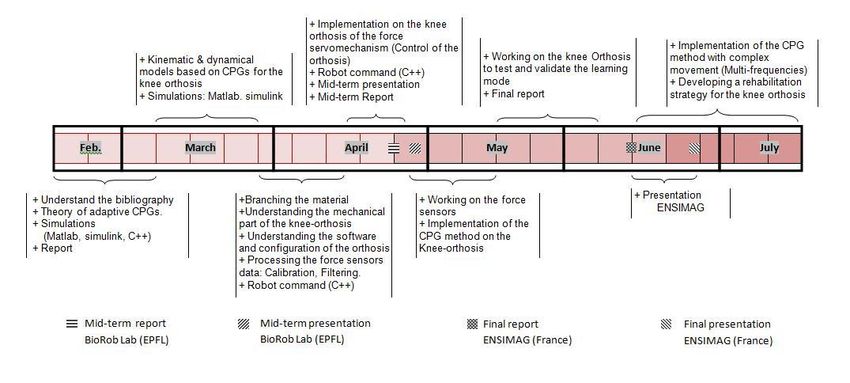
Abstract
Rehabilitation robotics is an application of engineering to design and develop technological
solutions for people suering from movement disorders. Nowadays, the existing rehabilitation
programs require many training sessions and sometimes up to three physiotherapists to move
one patient only. Therefore, rehabilitation robotics is a promising research avenue to take over
some of this time- and energy-consuming workload.
Since 2009, the BioRobotics Lab at EPFL (Switzerland) has started to investigate this
eld,
targeting the development of novel rehabilitation methods using advanced control techniques
As
rst goal, the lab focuses on the rehabilitation of locomotion (lower limb).
One of the control technique developed by the lab is based on adaptive oscillators, i.e. oscil-
lators equipped with an adaptive mechanism which enables to adapt their intrinsic frequency
to one of the frequency components of an input signal. This approach is thought to be of par-
ticular relevance in the
eld of locomotion rehabilitation, the arti
cial oscillator augmenting
the biological Central Pattern Generator (CPG). CPGs are neuronal oscillators located in the
spinal cord and producing coordinated multidimentional rhythmic signals, under the control
of simple inputs.
This thesis aims at investigating the way to integrate these adaptive oscillators into inno-
vative rehabilitation protocols. As initial validation, this method is implemented on a knee
orthosis, developed at the Laboratoire des Systèmes Robotiques (EPFL, Switzerland). It is
targeting the development of autonomous rehabilitation robots that can , for example, be
used at home as an extension of standard therapy. Based on results obtained for upper limb
assistance, our study pioneers the use of adaptive oscillators in lower limb rehabilitation.
In contrast to most standard protocols in rehabilitation robotics, where the reference
movement is pre-speci
ed by the therapist, this method permits the patient to choose the
frequency and amplitude of the intended movement, out of any constraint. The frequency
spectrum of the knee kinematics is learned by the coupled oscillators and makes the orthosis
able to synchronize with the movement, providing augmentation.
To validate the proposed method, a
rst study is conducted on a model created with
Simulink. This simulates the implementation in order to control and adjust the experimental
settings. The second stage is an actual validation using the knee orthosis. The test is made
with a target movement of increasing complexity:
rst, a single harmonic (sinusoidal), then
more complex signals with more then one frequency component.
Key words: Rehabilitation robotics, lower limbs paresis, Adaptive frequency oscillators,
Central Pattern Generator, knee orthosis
Rehabilitation robotics using Central Pattern Generators Biorob Lab
Acknowledgments
I want to express my deep gratitude to my supervisors: Mohamed BOURI and Renaud
RONSSE. I learnt a lot through them, not only scienti
cally, but also in the way to be a
researcher. This is something very precious that I will keep.
I would like to thank Prof. Auke J. Ijspeert for providing the opportunity to do my Master
thesis. It was a real pleasure to spend these few months in his Lab.
Special thanks to my ENSIMAG supervisor Florence Maraninchi, for her advice, guidance
and support.
Lastly, I thank my family, for their unconditional support and for providing a cheerful
atmosphere with constant encouragement.
Sarah MOUSSOUNI 2 Master project, summer 2010
Contents
1 Introduction                                                                                                               7
    1.1 Context of the project . . . . . . . . . . . . . . . . . . . .      .   .   .   .   .   .   .   .   .   .   .   .    8
    1.2 Environment : Presentation of the rehabilitation orthosis           .   .   .   .   .   .   .   .   .   .   .   .    9
    1.3 Project outline . . . . . . . . . . . . . . . . . . . . . . . .     .   .   .   .   .   .   .   .   .   .   .   .   10
        1.3.1 Project stages . . . . . . . . . . . . . . . . . . . . .      .   .   .   .   .   .   .   .   .   .   .   .   10
        1.3.2 Project schedule . . . . . . . . . . . . . . . . . . .        .   .   .   .   .   .   .   .   .   .   .   .   11
2 Adaptive oscillators                                                                                                      12
    2.1 Central Pattern Generators . . . . . . . . . . . . . . .    .   .   .   .   .   .   .   .   .   .   .   .   .   .   12
    2.2 Architecture of the adaptive oscillators . . . . . . . .    .   .   .   .   .   .   .   .   .   .   .   .   .   .   13
        2.2.1 Basic unit: Hopf Oscillator . . . . . . . . . . .     .   .   .   .   .   .   .   .   .   .   .   .   .   .   13
    2.3 Numerical simulations . . . . . . . . . . . . . . . . . .   .   .   .   .   .   .   .   .   .   .   .   .   .   .   13
        2.3.1 Learning a simple periodic signal . . . . . . . .     .   .   .   .   .   .   .   .   .   .   .   .   .   .   13
        2.3.2 Learning multi-frequency signals . . . . . . .        .   .   .   .   .   .   .   .   .   .   .   .   .   .   15
    2.4 Coupled Oscillators for learning multi-frequency signal     .   .   .   .   .   .   .   .   .   .   .   .   .   .   15
3   Model of the Knee active Orthosis                                                                                       17
    3.1 Dynamical model of a representative human lower limb . . . . . . .                      .   .   .   .   .   .   .   17
        3.1.1 Dynamical model . . . . . . . . . . . . . . . . . . . . . . . .                   .   .   .   .   .   .   .   17
        3.1.2 Position controller of the knee orthosis . . . . . . . . . . . .                  .   .   .   .   .   .   .   18
    3.2 Adaptive oscillator and augmentation estimator block . . . . . . .                      .   .   .   .   .   .   .   20
        3.2.1 The adaptive oscillator and signal estimator . . . . . . . . .                    .   .   .   .   .   .   .   20
        3.2.2 The augmentation estimator block . . . . . . . . . . . . . .                      .   .   .   .   .   .   .   22
    3.3 Simulations and Results . . . . . . . . . . . . . . . . . . . . . . . .                 .   .   .   .   .   .   .   22
        3.3.1 Simulation 1 : Simple stable sinusoidal movement . . . . . .                      .   .   .   .   .   .   .   22
        3.3.2 Simulation 2 : Sinusoidal movement with variable frequency                        .   .   .   .   .   .   .   23
4 Implementation of the method on the knee orthosis                                                                         25
    4.1 Step 1 : Implementation of the transparent mode . . . . . . . . . . . . . . . . 26
        4.1.1 Force calibration and curve interpolation . . . . . . . . . . . . . . . . . 26
        4.1.2 Force ltering . . . . . . . . . . . . . . . . . . . . . . . . . . . . . . . . 27
                                                3
Rehabilitation robotics using Central Pattern Generators                            Biorob Lab

       4.1.3 Characterization of the knee orthosis . . . . . . . . . . . . . . . . . . .       28
       4.1.4 Closed loop . . . . . . . . . . . . . . . . . . . . . . . . . . . . . . . . .     31
       4.1.5 Discussion . . . . . . . . . . . . . . . . . . . . . . . . . . . . . . . . . .    33
   4.2 Adaptive oscillator and augmentation torque . . . . . . . . . . . . . . . . . . .       33
       4.2.1 First stage: Validation of the learning block using a reference movement          34
       4.2.2 Results . . . . . . . . . . . . . . . . . . . . . . . . . . . . . . . . . . . .   35
       4.2.3 Second stage: Human movement . . . . . . . . . . . . . . . . . . . . . .          35
       4.2.4 Results and discussion . . . . . . . . . . . . . . . . . . . . . . . . . . . .    35
5 Conclusion                                                                                   36
6 References                                                                                   37

Sarah MOUSSOUNI                                4                 Master project, summer 2010
List of Figures
 1.1 Knee orthosis . . . . . . . . . . . . . . . . . . . . . . . . . . . . . . . . . . . . . 9
 1.2 Branching schema of the Knee orthosis system . . . . . . . . . . . . . . . . . . . 10
 1.3 Project schedule . . . . . . . . . . . . . . . . . . . . . . . . . . . . . . . . . . . 11
 2.1 Convergence of the frequency of an adaptive frequency oscillator driven by a
     signal F(t) = sin(20t) for dierent initial intrinsic frequencies . . . . . . . . . .       14
 2.2 Convergence of the adaptive oscillator frequency using dierent epsilon . . . . .           14
 2.3 Graph showing the convergence of the adaptive oscillator frequency to one of
     the frequencies components of the teaching signal . . . . . . . . . . . . . . . . .         15
 2.4 illustration of the multi-frequecies learning method . . . . . . . . . . . . . . . .        16
 2.5 Equation of the coupled oscillator to learn a multi-frequency signal . . . . . . .          16
 3.1 Figure showing the similarities between the pendulum and the knee-orthosis
     robot . . . . . . . . . . . . . . . . . . . . . . . . . . . . . . . . . . . . . . . . . .   18
 3.2 The PID controller implemented with the Simulink library . . . . . . . . . . . .            20
 3.3 Figure showing the adaptive oscillator and estimator blocks implemented in the
     Simulink model . . . . . . . . . . . . . . . . . . . . . . . . . . . . . . . . . . . .      21
 3.4 Evolution of the adaptive oscillator frequency . . . . . . . . . . . . . . . . . . .        22
 3.5 Evolution of the error of estimation: Current Position - Estimated position [deg]           23
 3.6 gure showing the evolution of the adaptive oscillator frequency to the two
     dierent frequencies of the input signal and the estimation of position which
     depend on the frequency adaptation . . . . . . . . . . . . . . . . . . . . . . . .          24
 4.1 Global schema of the rehabilitation system implementaed on the knee-orthosis .              25
 4.2 The graph represents the measured Force-voltage values and the spline inter-
     polation used to represent the curve . . . . . . . . . . . . . . . . . . . . . . . .        27
 4.3 The calibration of the measured force signal. The green signal corresponds
     to the measured voltage (Volt), The blue signal represents the calibrated and
     interpolated signal . . . . . . . . . . . . . . . . . . . . . . . . . . . . . . . . . .     27
 4.4 Curve of ltred signal, the green signal represent the tension measured by the
     force sensors. The blue signal is the corresponding force curve before applying
     the lter, the red curve is the ltered signal . . . . . . . . . . . . . . . . . . . .      28
                                              5
Rehabilitation robotics using Central Pattern Generators                              Biorob Lab

   4.6 Curve representing the measured tension (Volt) according to the input tension
        sent to the motor . . . . . . . . . . . . . . . . . . . . . . . . . . . . . . . . . .    29
   4.5 Figure showing the method used to x the orthosis arm. (1)(2) Pictures before
        xing the orthosis. (3)(4) Shows the xing method . . . . . . . . . . . . . . . .        29
   4.7 shows the curve displaying the tension sent according to the movement direction
        and the targeted position . . . . . . . . . . . . . . . . . . . . . . . . . . . . . .    30
   4.8 The function chosen to compute the required torque to send vs the direction
        and velocity of the movement . . . . . . . . . . . . . . . . . . . . . . . . . . . .     31
   4.9 Closed loop of the transparent mode . . . . . . . . . . . . . . . . . . . . . . . .       32
   4.10 In blue, the measured toque that the human provide to move the orthosis, in
        red, the computed torque using the previous formula with Kp = 1 . . . . . . .            32
   4.11 The three gures shows the human eort in three dirent cases :(1)Without
        transparent mode. force: [-4,4] Newton (2) With orthosis controller Kp=2.
        force: [-3,2] Newton (3) With orthosis controller and compensation torque
        Kp=2, force: [-2,1]Newton. [images from demonstration video] . . . . . . . . . .         33
   4.12 Simulation using an in blue signal in the top represents the frequency of the
        oscillator, The two other signals represent state variables x, y . The input signal
        frequency = 4 Hz . . . . . . . . . . . . . . . . . . . . . . . . . . . . . . . . . . .   34
   4.13 The gure shows the estimated position and velocity of the sent signal : in
        red (velocity) and blue(position) of the input signal , in bleu (velocity) and
        green(position) of the estimated signal . . . . . . . . . . . . . . . . . . . . . . .    35

Sarah MOUSSOUNI                                 6                  Master project, summer 2010
Chapter 1
Introduction
Rehabilitation robotics is a special branch of robotics which focuses on machines that
are used to help people to recover from severe physical trauma.1 There are many areas of
physical therapy where robots can provide support to the patients. One of these areas is the
rehabilitation of locomotion.
People suering from walking de
ciencies have better recovery expectancies using intensive
rehabilitation program. However, in standard rehabilitation process, many physiotherapists
often work with one patient to support limbs and help him/her to move at early stages. It is
time and energy consuming with many limitations. Then, rehabilitation robotics tools have
come out to overcome some of the physiotherapist's workload. Ref [4] [6]
These robots fall into two main classes: robots designed to compensate for lost skills,
including manipulation, self-feeding, or mobility; and those developed to cure or retrain lost
motor function after a disabling event such as stroke. Research on the eectiveness of robotic
therapy has shown that rehabilitation technologies provide new options for repetitive move-
ment training that can complement eorts to improve the therapy performance.
In that respect, our project goal is to investigate an innovative rehabilitation protocol
for locomotion using existing rehabilitation robots. This protocol is based on the theory of
Central Pattern Generators (CPG) and adaptive oscillators, which are non-linear oscillators
capable to synchronize with any periodic input. They are currently developed at the Biorob
Lab (EPFL). These oscillators can adapt their frequency without any signal processing or the
need to specify a time window or similar free parameters. They have been used to model
various biological processes and they are also used in engineering
elds, such as autonomous
robotics.
The major contribution of this thesis is to show that the method using adaptive oscillators
reduces the metabolic cost of the human performer and this for a simple movement viewed as
a sinusoidal signal to a multi-frequencies one.
1
www.wisegeek.com
7
Rehabilitation robotics using Central Pattern Generators Biorob Lab
The idea is the following: each moving joint can be viewed as an oscillator that is syn-
chronized with a second arti
cial oscillator, which in turn feeds some energy back to the user
through the robotics interface. This method provides some augmentation to the user as a
physiotherapist adds during the standard rehabilitation process. However, the robot leaves
all high-level parameters up to the patients, such as the movement amplitude and frequency.
The rehabilitation robots used were developed at the LSRO Lab (EPFL). The
rst ex-
ploration was done on a simple knee active orthosis oering one degree of freedom (1 DOF).
Later, this thesis will be the basis of a second exploration which will be done on the Lambda
robot oering 3 degrees of freedom per leg. Ref[7]
In this document, we will discuss the following points:
rstly, a short introduction of the
project context and environment is provided. The following chapter presents the adaptive
oscillator, its architecture and properties; and explains the innovation that can be made using
this method. The next part of the report describes the theoretical studies about the kinematic
and dynamical models of the lower limbs and the simulation made with Simulink platform
to validate the method. The last chapter describes the preliminary work done on the knee-
orthosis to test the rehabilitation method. Finally, the experimental results are provided with
a discussion about the future work that will be done in the next months, as an extension of
this thesis.
1.1 Context of the project
The following project is driven by a collaboration between the Biorobotics Laboratory
(Biorob Lab) providing methods and daily guidance, and the Laboratory of Robotics Systems
(LSRO) which provides robotics platforms and software support, both at EPFL, Switzerland.
My supervisors are Dr Renaud Ronse 2 , post-doctoral fellow at the Biorobotics Laboratory
(Directed by Professor Auke Ijspeert 3 ) and Dr Mohamed Bouri4 , the head of the parallel
robotics design group at the Laboratory of Robotics Systems (Directed by the Professor R.
Clavel).
The Biorobotics Laboratory (BioRob) is part of Institute of Bioengineering in the School
of Engineering at the EPFL. Its research interests are at the intersection between robotics,
computational neuroscience, nonlinear dynamical systems, and machine learning. One of their
recent
elds of investigation is rehabilitation robotics. They target to embed their research
in advanced control techniques (such as Central Pattern Generators -CPG-) and optimization
into robotics platforms providing rehabilitation therapy to disabled persons. Therefore, the
investigation of the rehabilitation of locomotion (lower limb), is one of the new objectives of
2
renaud.ronsse@ep
.ch
3
auke.ijspeert@ep
.ch
4
mohamed.bouri@ep
.ch
Sarah MOUSSOUNI 8 Master project, summer 2010Rehabilitation robotics using Central Pattern Generators Biorob Lab
the Lab and motivated this research project.
The LSRO Lab is a multidisciplinary research unit working mostly in the
elds of robotics,
micro-robotics and high precision instrumentation. One of their
elds of interest is medical
robotics and instrumentation. They work on robotics assistance to oer the possibility of
performing therapeutic mobilization treatments on paralyzed people and on a challenging lo-
comotor re-education project. The active Knee-orthosis is one of the rehabilitation prototypes
developed in the lab. It is used during this thesis as test platforms for the novel rehabilitation
method using adaptive oscillators.
1.2 Environment : Presentation of the rehabilitation orthosis
The work described in this thesis uses the the Knee-orthosis. The rehabilitation orthosis
(
gure 3.1) is used for simulation, validation of the method and for the proof of the concept.
It is provided by the LSRO Lab. It is a one-axis robotic arm allowing the mobilisaition of
the lower extremities and rehabilitation. It is able to control the
exion and extension of the
knee. It is a 1 DOF (Degree Of Freedom) robot.
The Electrical DC motor, an angular position sensor and a force sensor allow the total
instrumentation of the device. The used DC motor and the harmonic drive gear provide a
resistant torque as well as an assistive torque to implement dierent interaction strategies
between the leg and the orthosis arm. A joint torque up to 50Nm and a speed up to 110/s
may be obtained in the exercises.
Figure 1.1: Knee orthosis
The
gure 1.2 shows the branching schema of the knee orthosis. Where : the reducing
coe
cient n = 120, the torque is computed as following : Γaxle = Γmotor ∗ n and the motor is
commanded by an electric current ±10A provided by the ampli
er.
Sarah MOUSSOUNI 9 Master project, summer 2010Rehabilitation robotics using Central Pattern Generators Biorob Lab
Figure 1.2: Branching schema of the Knee orthosis system
1.3 Project outline
1.3.1 Project stages
The project is decomposed in
ve stages. In each stages, precise objectives are
xed and a
set of tasks have to be done to reach the
nal aim of the project. It is decomposed as following:
1. This stage aims at understanding the mathematical background of the adaptive CPGs
theory and reproduce simulations of the dierent articles in order to handle with these
tools. Matlab, SimuLink and C++ are used to implement and simulate the CPGs.
2. This part consists in deriving the kinematic and dynamical models of a representative
human lower body, and adapting the rehabilitation method based on adaptive CPGs
on this new con
guration with Knee orthosis. Simulation and
rst experiments will be
done on simulink and matlab.
3. This stage focuses on the derivation of a model of the geometrical con
guration of the
one degree of freedom knee active orthosis and on the programming of the robot interface
(C++).
4. A various experimentations will be done to simulate dierent human movement: sinu-
soidal and multi-frequency signals
5. To
nish, the whole implementation on robots will be tested on intact people.
Sarah MOUSSOUNI 10 Master project, summer 2010Rehabilitation robotics using Central Pattern Generators Biorob Lab
1.3.2 Project schedule
The
gure 1.3 shows the detailed project schedule and the work done during the
ve
months.
Figure 1.3: Project schedule
Sarah MOUSSOUNI 11 Master project, summer 2010Chapter 2
Adaptive oscillators
Nonlinear oscillators are widely used to model various physical and biological processes.
Specially in the modeling and control in the
eld of robotics. Oscillator models are interesting
because their ability to synchronize with other oscillators or with any input signal. In the case
of classical oscillators, it exists a phase-locking region around the intrinsic frequency delimiting
the basin of attraction of synchronization, because of, these oscillators cannot dynamically
adapt their parameters outside this region. It is di
cult to choose the right parameters of the
oscillator to ensure that it will synchronize as desired. ref [2][3] Some recent studies targeted
the development of oscillator able to adapt to a wider range of frequencies. The Biorob Lab
has designed adaptive oscillators whose frequency can be adapted to the frequency of periodic
input signals. It add a large contribution in the
eld of adaptive oscillators. In this chapter,
we will review this fame work of adaptive oscillators.
2.1 Central Pattern Generators
Central pattern generators are biological neural networks that produce coordinated mul-
tidimensional rhythmic signals, under the control of simple input signals.
Oscillators are ables to imitate CPGs. The new mechanism of adaptive oscillator using
coupled adaptive non-linear oscillators is able to learn arbitrary rhythmic signals. The intrin-
sic frequencies (ω) is automatically adjusted to replicate the teaching signal and one the signal
is removed the trajectory remains embedded into the dynamical system without an external
algorithm and can be played back.
the process is dynamic and can be applied to many kinds of teaching signals.
12Rehabilitation robotics using Central Pattern Generators Biorob Lab
2.2 Architecture of the adaptive oscillators
2.2.1 Basic unit: Hopf Oscillator
These oscillators are able to learn the frequency of complex periodic input signal without
any external optimization process.
To illustrate the frequency learning method, we describe the augmented Hopf oscillator
proposed in reference [2,3]. The frequency of the oscillator is used as a new state variable.
This variable will converge to one of the frequencies of the input signal. The frequency com-
ponent adapted will depend on the initial conditions for ω. The learning rule equations of
these oscillator are as follows:
ẋ = γ(µ − r2 )x − ωy + F (t) (2.1)
ẏ = γ(µ − r2 )y + ωx (2.2)
y
ω̇ = −F (t)( )
r
(2.3)
where r = x2 + y2 , µ controls the amplitude of the oscillator, γ controls the speed of
p
recovery after perturbation, is a coupling constant , F (t) is a periodic input to to which the
oscillator will adapt its frequency , ω is the frequency of the oscillator, which will be adapted
to the frequency of the input signal. In the case of multi-frequency signal, the oscillator will
converge to one of the frequencies. The adaptation has an in
nite basin of attraction. ref
[2][3]
2.3 Numerical simulations
2.3.1 Learning a simple periodic signal
As
rst example, we use the adaptive Hopf oscillator to learn a simple periodic signal.
Periodic functions are used to describe oscillations and waves. For example, the sine function
is periodic with period 2π. The period is the duration of one cycle in a repeating event, so the
period is the reciprocal of the frequency. In our example the frequency is equal to 20: The
teaching signal F (t) = sin(20t).
For the
rst experiment, the adaptive oscillator is tested with varying the initial intrinsic
frequency ω(0) = 5, 10, 20, 30, 35. This example will illustrate the ability of the oscillator
to adapt its frequency to the frequency of the input signal and will show the duration of this
adaptation.
Sarah MOUSSOUNI 13 Master project, summer 2010Rehabilitation robotics using Central Pattern Generators Biorob Lab
Figure 2.1: Convergence of the frequency of an adaptive frequency oscillator driven by a signal
F(t) = sin(20t) for dierent initial intrinsic frequencies
The
gure 2.1 shows that in all cases the oscillator is able to adapt it own frequency to
the frequency of the input signal and for the dierent ω(0). However, the synchronization
duration is dierent and depends on the initial frequency of the oscillator.
As a second simulation, we plots the evolution of ω for dierent values of =[0.2 , 0.5 ,
0.8, 1] using the teaching signalF (t) = sin(30t). ω(0)=35.
Figure 2.2: Convergence of the adaptive oscillator frequency using dierent epsilon
The
gure 2.2 clearly shows that the coupling constant determines the convergence speed
Sarah MOUSSOUNI 14 Master project, summer 2010Rehabilitation robotics using Central Pattern Generators Biorob Lab
of the oscillator around the teaching frequency. will be
xed at 1 as a default value.
2.3.2 Learning multi-frequency signals
1 To simulate the learning of multi-frequency signal, we used the following input :
F (t) = sin(10 ∗ t) + cos(25 ∗ t) + sin(32 ∗ t)
We will show through this example how the adaptive oscillator will converge and give a
formula to compute the frequency to which the oscillator will adapt its own ω. The following
gure plots the evolution of the intrinsic frequency of the adaptive oscillator when we have
dierent initial values of the state variables and illustrate the frequency component that attract
ω.
Figure 2.3: Graph showing the convergence of the adaptive oscillator frequency to one of the
frequencies components of the teaching signal
Remark: The adaptive oscillators are able to learn also the pseudo-periodic signals. see
ref [3].
2.4 Coupled Oscillators for learning multi-frequency signal
The basic idea is to use the adaptive property of the oscillators to learn the dierent
frequencies of a periodic teaching signal. It will be similar to dynamic Fourier series represen-
1
This section will be used in the future work on the multi-frequency movements. ref [1]
Sarah MOUSSOUNI 15 Master project, summer 2010Rehabilitation robotics using Central Pattern Generators Biorob Lab
tation, each oscillator will encode one frequency component of the learning signal.
The previous section showed that an adaptive oscillator is able to learn one frequency compo-
nent of a multi-frequency signal. Now, feedback is used to couple a set of adaptive oscillator
and to make each oscillator learning one frequency component of the teaching signal.
Figure 2.4: illustration of the multi-frequecies learning method
According to
gure 2.5, the equation 2.1, 2.2 and 2.3 will be adapted to the new learning
schema. The frequencies learned by the other oscillators will be considered and deleted from
the main teach signal. The equation are the following:
Figure 2.5: Equation of the coupled oscillator to learn a multi-frequency signal
More details are given in ref[1]
Sarah MOUSSOUNI 16 Master project, summer 2010Chapter 3
Model of the Knee active Orthosis
To implement and validate a reliable rehabilitation protocol, a computer simulation is used
rst to explore and gain new insights into adaptive oscillators. It estimates the performances
of the system and provides preliminary theoretical results.The whole system is modeled using
a Simulink Model for the control, parameter adjustment of the orthosis.
The study would like to prove that the adaptive oscillators provide augmentation to the
user and leave all high-level parameters of the movement up to him.
The system is decomposed into two main blocks. The
rst block is the mechanical model
of the orthosis and the human movement simulator. The second block is the learning and
augmentation block. It targets to integrate the adaptive oscillator to the global system and
study the learning method of the movement.
3.1 Dynamical model of a representative human lower limb
A
rst step consist in
nding an equivalent dynamical system to represent the human lower
limb and its interaction with the orthosis. This section provides a description of the lower
limb and orthosis modeling. The model provide the evolution of the orthosis position.
3.1.1 Dynamical model
The movement of the human using the knee orthosis has one degree of freedom. It moves
along a circular path. It is similar to the movement of a pendulum. Figure 3.1 shows the
similarities between the two systems.
The primary forces acting on the leg are the gravitational forces. In addition, there may be
a damping force from friction at the pivot. The model constructed describes how the angular
position θ of the orthosis varies as a function of time t. The gravitational force is directed
downward and has magnitude mg where g is the gravitational acceleration and m is the mass
17Rehabilitation robotics using Central Pattern Generators Biorob Lab
of the leg + the orthosis axle.The force acting in the tangential direction is −mgsin(θ). We
add damping to the model. We make the simplest possible assumption about the damping
force, that it is proportional to angular velocity, −b dθdt . In addition, the human provides a
torque u during its movement as an input.
The simple equation is written as follows:
I θ̈ = −mglsinθ − bθ̇ + u
Figure 3.1: Figure showing the similarities between the pendulum and the knee-orthosis robot
3.1.2 Position controller of the knee orthosis
The model of the human controller is a PID controller used to simulate the torque Uh (t)
provided by the human. The reference movement is a periodic function that can be changed
to simulate dierent desired movement. Using the dynamical model of human lower limb
described the previous section, the real-time position is provided and simulates the orthosis
sensors measurement.
A closed-loop feedback mechanism controlled by a PID minimizes the position error. It
adjusts the actual position with providing a torque according to this formula:
x
(3.1)
Z
d
Uh (t) = Kp e(t) + Ki e(t)dτ + Kd e(t)
0 dt
Sarah MOUSSOUNI 18 Master project, summer 2010Rehabilitation robotics using Central Pattern Generators Biorob Lab
where :
Proportional gain, Kp
Larger values typically mean faster response since the larger error is linked the proportional
term compensation. An excessively large proportional gain will lead to process instability and
oscillation.
Integral gain, Ki
Larger values imply steady state errors are eliminated more quickly. The trade-o is larger
overshoot: any negative error integrated during transient response must be integrated away
by positive error before reaching steady state.
Derivative gain, Kd
Larger values decrease overshoot, but slow down transient response and may lead to in-
stability due to signal noise ampli
cation in the dierentiation of the error.
Algorithm:
previousError = 0
integral = 0
start:
error = setpoint - actualPosition
integral = integral + (error*dt)
derivative = (error - previousError)/dt
output = (Kp*error) + (Ki*integral) + (Kd*derivative)
previousError = error
wait(dt)
goto start
Sarah MOUSSOUNI 19 Master project, summer 2010Rehabilitation robotics using Central Pattern Generators Biorob Lab
Figure 3.2: The PID controller implemented with the Simulink library
3.2 Adaptive oscillator and augmentation estimator block
The learning method using the adaptive oscillator and the computation of the orthosis
augmentation are provided in the following section. To
nish, some simulation are described
to show the validation of the method and the discussion made about the proposed solution.
The method developed in this work uses the adaptive oscillator presented in the previous
chapter and consists in learning the frequency of the human movement. It means that the
oscillator estimates and provides on each sampling period the corresponding x, y formula 2.1,
2.2 and ω formula 2.3 of the input signal. The input signal θ(t) is the orthosis-human position.
The next step consists in using the data provided by the oscillator to build an estimated
evolution of the human position, velocity and acceleration. This estimation makes able to
compute an estimated human torque.
The details of the implementation are given in the following sections and the rehabilitation
method is described in the last section provided by example of simulation results.
3.2.1 The adaptive oscillator and signal estimator
This part of the system is decomposed into two main blocks [see
gure 3.3 ]:
(1) The modi
ed Hopf oscillator which is the adaptive oscillator and which computes the
frequency of the input signal by adapting its own intrinsic frequency to this one.
(2) The position and movement characteristics estimator used to estimate the position,
velocity and acceleration of the orthosis and human leg.
Sarah MOUSSOUNI 20 Master project, summer 2010Rehabilitation robotics using Central Pattern Generators Biorob Lab
Figure 3.3: Figure showing the adaptive oscillator and estimator blocks implemented in the
Simulink model
(1) The adaptive oscillator
Using the Hopf adaptive oscillator system formula 2.1,2.2,2.3, an adaptive block was im-
plemented using the Simulink S-function standards [Appendix]. Additional variable α0 and
α1 corresponding respectively to the oset and amplitude of the signal are computed using
the evolution of the usual input variables of the adaptive oscillator.
α̇0 =
τ
2
F (t) (3.2)
α̇1 = τ xF (t) (3.3)
Where F (t) depends on the position the human leg (Orthosis) and the estimated position
computed by the next block F (t) = θ(t) − θ̂(t)
(2) The position and movement characteristics estimator
To estimate the position, velocity and acceleration of the movement, using the previous
results, the equations are as follows:
For the
rst study, we consider that the human movement is sinusoidal and can be estimated
thanks to the oset, amplitude and x position data as follows :
θ̂ = α0 + α1 x (3.4)
The velocity is simply computed using the amplitude , frequency and y position data. It
is the derivative of the estimated position.
ˆ
θ̇ = α1 ωy (3.5)
Sarah MOUSSOUNI 21 Master project, summer 2010Rehabilitation robotics using Central Pattern Generators Biorob Lab
The acceleration is the estimated velocity derivative. It is computed as following:
ˆ
θ̈ = α1 ω 2 x (3.6)
3.2.2 The augmentation estimator block
Using the previous results, an estimated user torque can be computed using the following
dynamical equation of the system:
ˆ ˆ
û = mglsin(θ̂) + bθ̇ + I θ̈ (3.7)
Where û is the estimated total torque of the system. û = ûHuman + ûOrthosisAugmentation
To provide an assistance, the torque provided by the human have to be estimated and
augmented to decrease his eort. The estimated torque û can be easily computed using the
result of the signal estimator for the θ̂, θ̇ˆ and θ̈ˆ [ See formula 3.4, 3.5, 3.6]. The augmented
torque will be a simple gain torque computed as follows:
uAugmentation = K ûHuman = K(û − ûOrthosisAugmentation ) (3.8)
Where K ∈ [0, 1[ speci
es the augmentation added to help the human to do the movement
with less eort.
3.3 Simulations and Results
3.3.1 Simulation 1 : Simple stable sinusoidal movement
As a
rst simulation, the user provides a stationary eort doing periodic sinusoidal move-
ment. The referent movement is a function de
ned as follows:
θ(t) = α ∗ sin(ω ∗ t)
Where α the amplitude is equal to π2 , ω the frequency of the movement is equal to 2π
Figure 3.4: Evolution of the adaptive oscillator frequency
Sarah MOUSSOUNI 22 Master project, summer 2010Rehabilitation robotics using Central Pattern Generators Biorob Lab
Figure 3.5: Evolution of the error of estimation: Current Position - Estimated position [deg]
Discussion
The
gure 3.4 shows that using an adaptive oscillator with an initial ω = 7 can, in less than 25
sec, adapt its frequency to the frequency of the input signal ω = 2π. In addition, the
gure 3.5
shows clearly the relation between the frequency adaptation and the position estimation. The
error of the estimated signal θ decreases during the oscillator adaptation stage and converges
to 0 when the oscillator learnt the signal frequency. In this case the estimator torque block
can easily compute the human torque and provide the desired augmentation according to the
formula 3.8. [Appendix [1][2] Simulink model]
3.3.2 Simulation 2 : Sinusoidal movement with variable frequency
In this simulation, the input signal is a sinusoidal one which the initial frequency ω = 2π
and after 40 sec decreases to ω = π. This means that the adaptive oscillator has to adapt its
intrinsic frequency respectively from 2π to π. The initial frequency of the oscillator is equal
to 7.
Sarah MOUSSOUNI 23 Master project, summer 2010Rehabilitation robotics using Central Pattern Generators Biorob Lab
Figure 3.6:
gure showing the evolution of the adaptive oscillator frequency to the two dierent
frequencies of the input signal and the estimation of position which depend on the frequency
adaptation
Discussion The
gure 3.6 shows that the adaptive oscillator adapts its frequency to
the frequency component of the signal in a very short time. The signal estimator using the
data providing by the oscillators estimates in parallel the correct characteristics of the user
movement and provides the estimated torque for each sampling time.
The results of the previous simulations show the ability of the learning block (adaptive
frequency + signal estimator) to learn the human movement in a short time and with an
error of estimation which converge to 0. This results validate our expectation of the system
performance. The next stage is the implementation and validation of the method on the knee
orthosis.
Sarah MOUSSOUNI 24 Master project, summer 2010Chapter 4
Implementation of the method on the
knee orthosis
In the previous chapters, the general method for designing the lower limb assistance using
adaptive oscillators was simulated and validated. Furthermore, it was shown that the method
provides a the expected results (signal estimation) for the sinusoidal movement.
This last chapter will discuss the dierent stages to implement and test the augmentation
method on the knee orthosis.
The work on the orthosis is decomposed into three mains stages: (1) Implementation of
the transparent mode stage (2) The learning stage (3) The torque augmentation stage. The
gure 4.1 shows the decomposition schema that will be detailed in the following chapter.
Figure 4.1: Global schema of the rehabilitation system implementaed on the knee-orthosis
25Rehabilitation robotics using Central Pattern Generators Biorob Lab
4.1 Step 1 : Implementation of the transparent mode
The objective of this preliminary work is to oer the transparent mode to the user, such
that the user will move the orthosis with a low perception of the mechanical impedance during
user-driven motions. [Appendix [4,5]]
4.1.1 Force calibration and curve interpolation
The preliminary work done on the orthosis consisted in calibrating the data transmitted
by the force sensor.
The force sensor provides an analogical value corresponding to the force voltage (Volt).
This data must be processed and calibrated to have an equivalent force value in Newton.
Therefore, a force calibration curve was constructed using a set of measurements.
The method of measurement is as follows: using a dynamometer, a device for measuring
force, the orthosis is initialized on the vertical position (0) . A set of force value in a range of
[-5, 10] KgN is applied on the orthosis. The voltage measured by the force sensors makes able
to draw the calibration curve. This curve provides the correspondence between any voltage
(Volt) measured and the force value in (Newton). See
gure 4.2.
To construct the
nal Force-voltage curve, the Spline quadratic interpolation method was
implemented in C++ and used on the range of the discrete measurements done using the
dynamometer. The Spline interpolation uses low-degree polynomials in each of the intervals,
and chooses the polynomial pieces such that they
t smoothly together [code in the Appendix
[3]].
Force -5 -4 -3 -2 -1 0
Tension -0.85 -0.75 -0.67 -0.55 -0.41 -0.23
Force 1 2 3 4 5 6 7 8 10
Tension -0.1 0 0.1 0.2 0.37 0.58 0.65 0.77 0.96
Sarah MOUSSOUNI 26 Master project, summer 2010Rehabilitation robotics using Central Pattern Generators Biorob Lab
Figure 4.2: The graph represents the measured Force-voltage values and the spline interpola-
tion used to represent the curve
Discussion
The curve constructed from the set of measurements has some interfering signal noise. The
next step is signal
ltering. It targets removing some frequencies and suppressing interfering
noise.
Figure 4.3: The calibration of the measured force signal. The green signal corresponds to the
measured voltage (Volt), The blue signal represents the calibrated and interpolated signal
4.1.2 Force
ltering
The next stage in processing the measured force is the
ltering process. It is used to
eliminate unwanted frequencies from the received signal. While the correct
lter settings can
signi
cantly improve the visibility of a defect signal, incorrect settings can distort the signal
presentation and even eliminate the defect signal completely. Therefore, it is important to
understand the concept of signal
ltering. The
lter used is a low Pass Filter. It is adjusted
in Hertz (Hz). It was calculated as following:
Sarah MOUSSOUNI 27 Master project, summer 2010Rehabilitation robotics using Central Pattern Generators Biorob Lab
yf 1
=
y 1 + τs
τ yf τ yf−
=> yf + −
Te Te
τ τ −
=> (1 + )yf = yf + y
Te Te
Te + τ τ Te
=> ( )yf = yf− + y
Te Te Te
τ Te
=> yf = yf− + y
Te + τ Te + τ
Where yf is the
ltered signal, y is the measured signal, yf− is the previous value of the
signal, Te is the sampling time, τ = B1 , where Bp is the bandwidth, Bp = 20 Hz
p
Results : The following
gure illustrate the
ltering result.
Figure 4.4: Curve of
ltred signal, the green signal represent the tension measured by the
force sensors. The blue signal is the corresponding force curve before applying the
lter, the
red curve is the
ltered signal
4.1.3 Characterization of the knee orthosis
This section targets to study the characterization of the orthosis. It is used in the estima-
tion of the gravitational and dry friction torque of the orthosis.
Force measured for a speci
c tension curve
This study targets to measure the force applied on the orthosis arm when a de
ned tension
is sent. The method is the following: The orthosis arm is
xed to the position (0)[ see
g
4.5 ] and a tension increasing from -4 Volt to +5 Volt is sent. Fixed, the orthosis arm cannot
move and the force sensors will be able to measure the force applied by the motor on the
orthosis arm. The following table details the measurements done on the orthosis (See
g 4.6).
Sarah MOUSSOUNI 28 Master project, summer 2010Rehabilitation robotics using Central Pattern Generators Biorob Lab
Figure 4.6: Curve representing the measured tension (Volt) according to the input tension
sent to the motor
Applied Tension -4 -3 -2 -1 0 1 2 3 4 5
ADC measured -1.40 -0.90 -0.70 -0.30 +0.29 +0.90 +1.80 +1.40 +2.16 +2.80
Figure 4.5: Figure showing the method used to
x the orthosis arm. (1)(2) Pictures before
xing the orthosis. (3)(4) Shows the
xing method
.
Characterization of the static torque of the knee orthosis
In a
exion or extension movement, the subject using the orthosis will be confronted to
external forces which will disturb the user movement and increase its eort to move the orthosis
arm. Therefore, here, we compute the required input voltage to reach a position which is not
the vertical one.
For this experiment a set of eleven position are chosen in the [-60, +20] range. Each
10 , the corresponding sent tension is registered in both direction (
exing(High-bottom)-
Sarah MOUSSOUNI 29 Master project, summer 2010Rehabilitation robotics using Central Pattern Generators Biorob Lab
extension (Bottom-high) ). See
gure 4.7. The results are providing in the following table:
θ -60 -50 -40 -30 -20 -10 0 10 20
Flexing -0.27 -0.26 -0.24 -0.2300 -0.1800 -0.16 -0.120 -0.10 -0.08
Extension -0.05 -0.06 -0.04 -0.0106 -0.0156 0.02 0.052 0.10 0.16
Figure 4.7: shows the curve displaying the tension sent according to the movement direction
and the targeted position
Discussion
The obtained curves show that the required torque when the human is doing in
exion or
extension movement is dierent. The gravitational force in a position is the same when we
do a
exion or extension movement. It is linked to the position and not to the velocity
or acceleration. So, the dierence between the two curves is due to the dry friction which
in
uences with dierent degree the orthosis arm depending on the movement direction. It
means when we are in
exion movement. The orthosis arm is reaching the vertical position
(0). The required torque is smaller than the torque when the orthosis is going up doing a
extension movement.
To eliminate the gravitational and dry friction forces when the user is using the orthosis,
a torque Γ is added to overcome the in
uence of this forces. It is computed as follows:
Each measurement is done according to a sampling period SamplingP eriod = 0.0002.
Where the incrementation of the velocity during one sampling period is Resv = SamplingP
Res
eriod ,
θ
we consider that the maximum velocity ω = 5 ∗ Resv , the minimum velocity ω = −ω and
+ − +
the current velocity ωcurrent = SamplingP
θ −θ
current
eriod .
old
Using this data, the torque is estimated thanks to the previous measurements and accord-
ing to the following algorithm:
Algorithm :
Sarah MOUSSOUNI 30 Master project, summer 2010Rehabilitation robotics using Central Pattern Generators Biorob Lab
if ( ωcurrent ≤ ω− ) then
Γ = Γ− ;
else if ( ωcurrent ≥ ω+ ) then
Γ = Γ+ ;
else
Γ= Γ+ −Γ−
ω + −ω −
;
Where Γ+ is the torque measured when it is a
exing movement, Γ− is the torque mea-
sured when it is a extension movement. See
gure 4.8
Figure 4.8: The function chosen to compute the required torque to send vs the direction and
velocity of the movement
4.1.4 Closed loop
To make the user able to move the orthosis with a low perception of the mechanical
impedance during user-driven motions, a closed loop is implemented using the previous results
and providing an additional torque which will drive the interaction force between the human
and the orthosis to zero : Finteraction → FDesired = 0. To reach this objective, the orthosis is
provided by a PID controller.
The
gure 4.9 shows the global schema of the transparent mode which will be detailed
the following sections.
Sarah MOUSSOUNI 31 Master project, summer 2010Rehabilitation robotics using Central Pattern Generators Biorob Lab
Figure 4.9: Closed loop of the transparent mode
Force control with proportional gain
As a
rst experiment. the closed loop use only a proportional gain Kp . The providing
torque Uapp is computed using the eects of a closed feedback loop. It means that the measured
force provided by the force sensors is used to reach the desired one FDesired = 0 as following:
Uapp = Kp [Fdesired − Fmeasured ]
The following
gure illustrate the torque sent to decrease the human eort to move the
orthosis. The proportional gain Kp = 1. It means that the orthosis must provide the same
force provided by the user to have Finteraction → FDesired = 0.
Figure 4.10: In blue, the measured toque that the human provide to move the orthosis, in red,
the computed torque using the previous formula with Kp = 1
Sarah MOUSSOUNI 32 Master project, summer 2010Rehabilitation robotics using Central Pattern Generators Biorob Lab
Force control with a proportional and integral gain
In this closed loop the provided torque Uapp used the eects of a closed feedback loop
with the measured force and the desired one. The measurement error F is de
ned by :
F = Tdesired − Tmeasured . So, the provided torque is computed by the following equation:
Z t
Uapp = Kp F − Ki F (t)dt
0
Where Ki is the integral gain
4.1.5 Discussion
Using the closed loop in addition to the estimated torque, the orthosis moves freely and
the human eort decreased considerably. Figure 4.11 shows that the human eort when the
orthosis is without the transparent mode is larger than using the closed loop. The third curve
illustrate the eect of the additional gravitational torque to decrease the human force.
The transparent mode makes us able to implement the learning block and to start the study
of the rehabilitation method.
Figure 4.11: The three
gures shows the human eort in three dirent cases :(1)Without
transparent mode. force: [-4,4] Newton (2) With orthosis controller Kp=2. force: [-3,2]
Newton (3) With orthosis controller and compensation torque Kp=2, force: [-2,1]Newton.
[images from demonstration video]
4.2 Adaptive oscillator and augmentation torque
The validation of the transparent mode makes the user able to do its movement without
any additional eorts. The learning mode can be at this stage implemented and integrated to
the whole rehabilitation system.
The goal of this section is to describe the dierent stages to implement, test and validate
the new rehabilitation protocol using the adaptive oscillator.
The learning block was implemented in C++ [Appendix [6]]. A
rst part details the
preliminary test to validate the learning-block using a reference movement with a known
Sarah MOUSSOUNI 33 Master project, summer 2010Rehabilitation robotics using Central Pattern Generators Biorob Lab
amplitude and frequency. Afterwards, a second step provides the results of the learning
protocol using the movement of a subject using the orthosis. To
nish, the whole torque
estimation and rehabilitation protocol validation are described with dierent experimentations
done with a subject.
4.2.1 First stage: Validation of the learning block using a reference move-
ment
To validate the learning block, as a
rst experimentation. A
rst routine was write to send
a reference torque. This provided torque is a simple sinusoidal signal. This torque makes the
movement of the orthosis leg similar to the movement of a pendulum
g 4.12. The following
function describes the sent torque:
T orque(t) = αsin(ωt)
Where: α is the amplitude of the signal, ω frequency of the signal
Figure 4.12: Simulation using an in blue signal in the top represents the frequency of the
oscillator, The two other signals represent state variables x, y . The input signal frequency =
4 Hz
The simulation is using an input signal F (t) = αsin(ωt) with α = 3 and ω = 4, the blue
signal in the top represents the frequency of the oscillator, The two other signals represent
the xy state variables.
The experimentations consists on sending sequentially a various frequency and prove the
ability to adapt the intrinsic frequency of the oscillator with the input one. The Hopf adaptive
oscillator is tested with dierent signal frequency.
Sarah MOUSSOUNI 34 Master project, summer 2010Rehabilitation robotics using Central Pattern Generators Biorob Lab
4.2.2 Results
The adaptive oscillator is able to adapt its frequency to the input signal. The position of
the orthosis and the movement velocity and acceleration are correctly estimated and as shown
in the
gure 4.13
Figure 4.13: The
gure shows the estimated position and velocity of the sent signal : in red
(velocity) and blue(position) of the input signal , in bleu (velocity) and green(position) of the
estimated signal
4.2.3 Second stage: Human movement
In this section stage the test is made on the orthosis in interaction with a human. The
subject is asked to provide a movement. It is a periodic
exion/extension movement.
To ensure that the amplitude is same (±error ), the user must repeat the same movement
with the same velocity in this limited space [- 20, + 20 ].
The augmentation block is used to reduce the human eort uses an augmentation K = 0.5.
uAugmentation = K ûHuman = K(û − ûOrthosisAugmentation )
4.2.4 Results and discussion
The adaptive oscillator is able to follow the human movement and to reproduce the signal
characteristics (position, velocity and acceleration). During the experiment, the user changed
the frequency of its movement and the test results showed that the assistance system takes a
short time to learn the input signal and to provide the augmentation that the human need.
The system has enough time to follow the movement and the user move the orthosis with a
low perception of the augmentation system process.
Sarah MOUSSOUNI 35 Master project, summer 2010Chapter 5
Conclusion
The main goal of this study was to investigate a rehabilitation protocol based on the
theory of adaptive oscillators. The major contribution of this thesis was to propose a solution
to make the orthosis transparent for the user by creating a transparent mode and to study
the augmentation strategy to reduce the human eort.
The work was decomposed into two main stages. To implement and validate a reliable
rehabilitation system, a computer simulation was
rstly used to explore and gain new insights
into the use of this new technology of adaptive oscillator. It made us able to estimate the
performance of the system and to have preliminary theoretical results.The whole system was
modeled using Simulink for the control and adjustment of the orthosis. The second stage tar-
geted the implementation of the rehabilitation method on the Knee orthosis and the validation
of the on-line learning of the movement and the device augmentation. A set of experiments
was done to validate the rehabilitation method. The
rst one consisted to provide a refer-
ence movement to the orthosis. This movement was previously tested in the Simulink model
which made us able to compare the simulation results with the orthosis on-line learning and
augmentation. The second experiment was done on a user which provide a movement . The
subject tested
rstly the orthosis without any assistance and compared it the augmentation
mode.
This study made us able to investigate and validate the rehabilitation method on the knee
orthosis and to demonstrate the feasibility of using adaptive oscillators for human augmen-
tation. Similar experiments will be realized using EMG to have the precise evolution of the
participant eort during the assistance stage. Also, the next step in this thesis will be to
generalize the study to complex signals such as multi-frequencies movement. The experimen-
tations will be done during the next month and the results will make a major contribution to
the investigation of the rehabilitation method using adaptive oscillators. As future work, this
study will be extended to a more complex robot as the Lambda robot oering 3 degrees of
freedom per leg.
36Chapter 6
References
[1] L. Righetti and A. J. Ijspeert. Programmable central pattern generators: an ap-
plication to biped locomotion control. In Proc. IEEE International Conference on Robotics
and Automation ICRA 2006, pages 1585 1590, 2006. doi:10.1109/ROBOT.2006.1641933.
[2] J. Buchli, L. Righetti and A. J. Ijspeert . Frequency analysis with coupled non-
linear oscillators. Physica D, 237: 1705..1718, 2008.
[3] L. Righetti, J. Buchli and A. J. Ijspeert. Dynamic hebbian learning in adaptive
frequency oscillators. Physica D, 216: 269..281, 2006.
[4] A. Dollar and H. Herr. Lower extremity exoskeletons and active orthoses: Chal-
lenges and state-of-the-art. IEEE Transactions on Robotics, 24(1): 144 ..158, 2008. ISSN
1552..3098. doi: 10.1109/TRO.2008.915453.
[5] A. Gams, A. J. Ijspeert, S. Schaal and J. Lenarcic. On-line learning and modu-
lation of periodic movements with nonlinear dynamical systems. Auton Robot, 27: 3..23, 2009.
[6] S. Hesse, H. Schmidt, C. Werner and A. Bardeleben. Upper and lower ex-
tremity robotic devices for rehabilitation and for studying motor control. Curr Opin Neurol,
16(6): 705..710, 2003. doi:10.1097/01.wco.0000102630.16692.38.
[7] M. Bouri, Member, IEEE, B. Le Gall, R. Clavele. A new concept of parallel
robot for rehabilitation and
tness: The Lambda
37Rehabilitation robotics using Central Pattern Generators Biorob Lab
Appendix
Sarah MOUSSOUNI 38 Master project, summer 2010XY Graph
W_Curve x_Curve y_Curve Current_Estimated_Position
Clock
w
Error
t multi_freq y PosOrthese
x
Time
Subtract
50 Kp y
Reference_Mvt_Sujet
Out1 Torque PosHumain
Kp EstimatedPosition
2 Kd
EstimatedTorque 10
Kd Force TeachingSignal
5 Ki alpha1 Gain
Ki1 PID alpha0
Knee_Orthosis
Adaptive_Block
alpha0_Curve alpha1_Curve TorqueEstimator_Curve
Reference_Curve Error Torque Uh Force_Curve Position_Humain Position_OrthosisF:\ARCHIVE RTX\RtxController_12June2010\Interpolation.cpp 1
ANNEX : [3]
/*---------------------------------------------------------------*
* PROJET : Rehabilitation robotics using CPG
*---------------------------------------------------------------*
Author : Sarah MOUSSOUNI
Supervisor : Mohamed BOURI (LSRO Lab)
Renaud RONSSE (BioRob Lab)
Date : Feb - July 2010
EPFL : Ecole Polytechnique Federale de Lausanne
*--------------------------------------------------------------*/
#include "Interpolation.h"
#include "math.h"
/*==========================*/
/* Interpolation */
/*==========================*/
//****************************************************************************80
void interval ( int n, double x[], double xval, int *left, int *right )
//****************************************************************************80
//
// Purpose:
// interval searches a sorted array for successive brackets of a value.
// Discussion:
// If the values in the vector are thought of as defining intervals
// on the real line, then this routine searches for the interval
// nearest to or containing the given value.
//
// It is always true that RIGHT = LEFT+1.
//
// If XVAL < X[0], then LEFT = 1, RIGHT = 2, and
// XVAL < X[0] < X[1];
// If X(1)You can also read