Online Robust Non-negative Dictionary Learning for Visual Tracking
←
→
Page content transcription
If your browser does not render page correctly, please read the page content below
Online Robust Non-negative Dictionary Learning for Visual Tracking

                             Naiyan Wang†            Jingdong Wang‡             Dit-Yan Yeung†
               †                                                                              ‡
                   Hong Kong University of Science and Technology                                 Microsoft Research
                      winsty@gmail.com           jingdw@microsoft.com              dyyeung@cse.ust.hk

                         Abstract
   This paper studies the visual tracking problem in video
sequences and presents a novel robust sparse tracker under                      (a) davidin                        (b) bolt
the particle filter framework. In particular, we propose an          Figure 1. Learned templates for two video sequences: davidin and
online robust non-negative dictionary learning algorithm             bolt. For each sequence, the learned templates cover different ap-
for updating the object templates so that each learned tem-          pearances of the tracked object in the video while rejecting the
plate can capture a distinctive aspect of the tracked object.        cluttered background.
Another appealing property of this approach is that it can
automatically detect and reject the occlusion and cluttered
                                                                     L1T describes the tracking target using basis vectors which
background in a principled way. In addition, we propose
                                                                     consist of object templates and trivial templates, and recon-
a new particle representation formulation using the Huber
                                                                     structs each candidate (particle) by a sparse linear combi-
loss function. The advantage is that it can yield robust esti-
                                                                     nation of them. While object templates correspond to the
mation without using trivial templates adopted by previous
                                                                     normal appearance of objects, trivial templates are used to
sparse trackers, leading to faster computation. We also re-
                                                                     handle noise or occlusion. Specifically, each trivial template
veal the equivalence between this new formulation and the
                                                                     has only one nonzero element being one for a specific fea-
previous one which uses trivial templates. The proposed
                                                                     ture. If it is selected to represent the particle, it means that
tracker is empirically compared with state-of-the-art track-
                                                                     the corresponding feature is occluded. It is shown in [18]
ers on some challenging video sequences. Both quantita-
                                                                     that a good target candidate should involve fewer trivial
tive and qualitative comparisons show that our proposed
                                                                     templates while keeping the reconstruction error low. We
tracker is superior and more stable.
                                                                     review the L1T in detail in section 3.2.
                                                                         In this paper, we present an online robust non-negative
1. Introduction                                                      dictionary learning algorithm for updating the object tem-
    Visual tracking or object tracking in video sequences            plates. The learned templates for two video sequences are
is a major topic in computer vision and related fields. It           shown in Fig. 1. We devise a novel online projected gradient
has a wide range of real-world applications, including secu-         descent method to solve the dictionary learning problem. In
rity and surveillance, autonomous vehicles, automatic traf-          contrast to the ad hoc manner by replacing the least used
fic control, medical imaging, human-computer interaction,            template with the current tracking result as in [18, 30], our
and many more. A typical setting of the problem is that              algorithm blends the past information and the current track-
an object identified, either manually or automatically, in           ing result in a principled way. It can automatically detect
the first frame of a video sequence is tracked in the subse-         and reject the occlusion and cluttered background, yielding
quent frames by estimating its trajectory as it moves around.        robust object templates. Besides, we formulate the particle
While the problem is easy to state, it is often challenging to       representation problem using the Huber loss function [10].
build a robust object tracker due to various factors which           This formulation can yield robust estimation without using
include noise, occlusion, fast and abrupt object motion, il-         trivial templates and thus lead to significant reduction of the
lumination changes, and variations in pose and scale. The            computational cost. Moreover, we also establish the equiv-
focus of this paper is on the widely-studied single object           alence between this new formulation and the L1T.
tracking problem.
    Mei and Ling proposed the `1 tracker (L1T) [18] for ro-          2. Related Work
bust visual tracking under the particle filter framework [5]
based on the sparse coding technique [22]. L1T and its ex-             Object tracking is an extensively studied research topic.
tensions [30, 29] showed promising results in various tests.         For a comprehensive survey of this topic, we refer readers

                                                                 1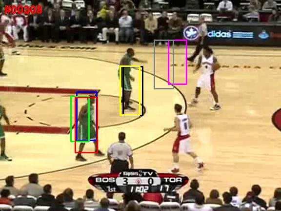
to the survey paper [26] and a recent benchmark [24]. Here       complicated environments, discriminative trackers are often
we only review some representative works which are cat-          more robust than generative trackers because discriminative
egorized into two approaches for building object trackers,       trackers use negative samples to avoid the drifting problem.
namely, generative and discriminative methods.                   A natural attempt is to combine the two approaches to give
    Generative trackers usually learn an appearance model        a hybrid approach, as in [31].
to represent the object being tracked and make decision              Besides object trackers, some other techniques related to
based on the reconstruction error. Incremental visual track-     our proposed method are (online) dictionary learning and
ing (IVT) [20] is a recent method which learns the dynamic       (robust) non-negative matrix factorization (NMF). Dictio-
appearance of the tracked object via incremental principal       nary learning seeks to learn from data a dictionary which is
component analysis (PCA). Visual tracking decomposition          an adaptive set of basis vectors or atoms, so that each data
(VTD) [15] decomposes the tracking problem into several          sample is represented by a sparse linear combination of the
basic motion and observation models and extends the con-         basis vectors. It has been found that dictionaries learned this
ventional particle filter framework to allow different basic     way are more effective than off-the-shelf ones (e.g., based
models to interact. The method that is most closely related      on Gabor filters or discrete cosine transform) for many vi-
to our paper is L1T [18] which, as said above, assumes that      sion applications such as denoising [1] and image classi-
the tracked object can be represented well by a sparse linear    fication [25]. Most dictionary learning methods are based
combination of object templates and trivial templates. Its       on K-SVD [1] or online dictionary learning [17]. As for
drawback of having high computational cost has been al-          NMF [21], it is a common data analysis technique for high-
leviated by subsequent works [19, 4] to improve the track-       dimensional data. Due to the non-negativity constraints,
ing speed. More recently, Zhang et al. found that consider-      it tends to produce parts-based decomposition of images
ing the underlying relationships between sampled particles       which facilitates human interpretation and yields superior
could greatly improve the tracking performance and pro-          performance. There are also some NMF variants, such as
posed the multitask tracker (MTT) [30] and low rank sparse       sparse NMF [9] and robust NMF [14, 6]. Online learning of
tracker (LRST) [29]. In [11], Jia et al. proposed using align-   basis vectors under the robust setting has also aroused a lot
ment pooling in the sparse image representation to alleviate     of interest, e.g., [23, 16].
the drifting problem. For a survey of sparse coding based
trackers, we refer readers to [28].                              3. Background
    Unlike the generative approach, discriminative trackers
formulate object tracking as a binary classification prob-           To facilitate the presentation of our model in the next
lem which considers the tracked object and the background        section, we first briefly review in this section the particle
as belonging to two different classes. One example is            filter approach for visual tracking and the `1 tracker (L1T).
the online AdaBoost (OAB) tracker [7] which uses online          3.1. Particle Filters for Visual Tracking
AdaBoost to select features for tracking. The multiple in-
stance learning (MIL) tracker [3] formulates object track-           The particle filter approach [5], also known as a sequen-
ing as an online multiple instance learning problem which        tial Monte Carlo (SMC) method for importance sampling, is
assumes that the samples belong to the positive or negative      commonly used for visual tracking. Like a Kalman filter, a
bags. The P-N tracker [12] utilizes structured unlabeled         particle filter sequentially estimates the latent state variables
data and uses an online semi-supervised learning algorithm.      of a dynamical system based on a sequence of observations.
A subsequent method called Tracking-Learning-Detection           The main difference is that, unlike a Kalman filter, the latent
(TLD) [13] augments it by a detection phase, which has the       state variables are not restricted to the Gaussian distribution,
advantage of recovering from failure even after the tracker      not even distribution of any parametric form. Let st and
has failed for an extended period of time. The Struck [8]        yt denote the latent state and observation, respectively, at
learns a kernelized structured output support vector ma-         time t. A particle filter approximates the true posterior state
chine online. It ranks top in the recent benchmark [24].         distribution p(st | y1:t ) by a set of samples {sti }ni=1 (a.k.a.
The compressive tracker (CT) [27] utilizes a random sparse       particles) with corresponding weights {wit }ni=1 which sum
compressive matrix to perform efficient dimensionality re-       to 1. For the state transition probability q(st+1 | s1:t , y1:t ),
duction on the integral image. The resulting features are        it is often assumed to follow a first-order Markov process
like generalized Haar features which are quite effective for     so that it can be simplified to q(st+1 | st ). In this case,
classification.                                                  the weights are updated as wit+1 = wit p(yt | sti ). In case
    Generally speaking, when there is less variability in the    the sum of weights of the particles before normalization is
tracked object, generative trackers tend to yield more accu-     less than a prespecified threshold, resampling is needed by
rate results than discriminative trackers because generative     drawing n particles from the current particle set in propor-
methods typically use richer features. However, in more          tion to their weights and then resetting their weights to 1/n.
                                                                     In the context of object tracking, the state si is often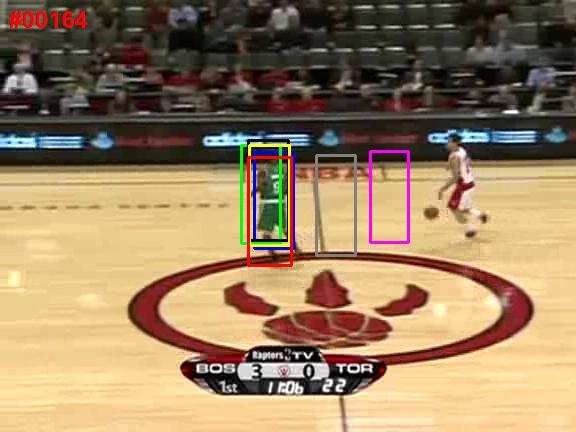
characterized by six affine parameters which correspond to            ing which represents each particle using the dictionary tem-
translation, scale, aspect ratio, rotation and skewness. Each         plates by solving an optimization problem that involves the
dimension of q(st+1 | st ) is modeled by an independent               Huber loss function. The second part is dictionary learning
Gaussian distribution. The tracking result at each time step          which updates the object templates over time.
is taken to be the particle with the largest weight. A key
issue in the particle filter approach is to formulate the ob-         4.1. Robust Particle Representation
servation likelihood p(yt | sti ). In general, it should reflect         In terms of particle representation, we solve the follow-
the similarity of a particle and the object templates while           ing robust sparse coding problem based on the Huber loss:
being robust against occlusion or appearance changes. We                                        XX
will discuss this issue in greater depth later in section 5.1.           min f (V; U) =                     `λ (yij − u0i· vj· ) + γkVk1
                                                                           V
    The particle filter framework is popularly used for vi-                                     i       j                                    (2)
sual tracking due partly to its simplicity and effectiveness.             s.t.   V ≥ 0,
First, as said before, this approach is more general than us-         where yij is an element of Y, ui· and vj· are column vectors
ing Kalman filters because it is not restricted to the Gaussian       for the ith row of U and jth row of V, respectively, and
distribution. Also, the accuracy of the approximation gener-          `λ (·) denotes the Huber loss function [10] with parameter
ally increases with the number of particles used. Moreover,           λ, which is defined as
instead of using point estimation which may lead to overfit-                               (
                                                                                             1 2
ting, the probability distribution of the latent state variables                               r           |r| < λ
                                                                                   `λ (r) = 2                                  (3)
is approximated by a set of particles, making it possible for                                λ|r| − 12 λ2 otherwise.
the tracker to recover from failure. An excellent tutorial on
using particle filters for visual tracking can be found in [2].          The Huber loss function is favorable here since it grows
                                                                      more slowly than the l2 norm as the residue increases, mak-
3.2. The `1 Tracker (L1T)                                             ing it less insensitive to outliers. Moreover, since it is
    In each frame, L1T first generates candidate particles            smooth around zero, it is more stable than the l1 norm when
based on the particle filter framework. Let Y ∈ Rm×n                  there exists small but elementwise noise. It encourages each
denote the particles with each of the n columns for one par-          candidate particle to be approximated by a sparse combina-
ticle. We further let U ∈ Rm×r denote the object templates            tion of the object templates and yet it can still accommodate
and V ∈ Rn×r and VT ∈ Rn×m denote the coefficients                    outliers and noise caused by occlusion and the like.
for the object templates and trivial templates, respectively.         Optimization: To minimize f (V; U) w.r.t. V subject to
For sparse coding of the particles, L1T solves the following          the non-negativity constraint V ≥ 0, we use the following
optimization problem:                                                 update rule:
                              V0

          1                             2
                                                                                                  p           0

  min       Y − [U Im ]                     + λkVT k1 + γkVk1                     p+1    p
                                                                                                            (W     Y) U      jk
 V,VT     2                   VT0       F                       (1)              vjk  = vjk h                             0 i           ,   (4)
                                                                                                Wp           (U(Vp )0 )    U        +γ
   s.t.   V ≥ 0,                                                                                                               jk

where Im denotes the identity matrix of size mP× m which              where the superscript p denotes the pth iteration of the opti-
corresponds to the trivial templates, kAk1 = ij |aij | for            mization procedure for V, denotes the Hadamard product
                                                                      (or called elementwise product) of matrices, and each ele-
the `1 norm, and kAkF = ( ij a2ij )1/2 for the Frobenius
                               P
                                                                      ment wij of W, representing the weight for the jth feature
norm. Then the weight of each particle is set to be inversely
                                                                      of particle i, is defined as
proportional to the reconstruction error. In each frame, the
particle with the smallest reconstruction error (and hence                                          (
                                                                                                        1          p
                                                                                                                 |rij |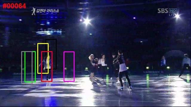
Connection to the trivial templates: Our approach based                   target for an extended period of time and allow them to de-
on the Huber loss function is actually related to the popular             cay slowly, since it helps a lot in recovering from occlusion.
approach using trivial templates as in Eqn. 1. First, Eqn. 1              As shown in Fig. 1, the learned templates summarize well
can be expressed equivalently in the following form:                      different appearances of the target in the previous frames.
                 1                                                        Optimization: To solve this optimization problem, as is
                                        2
         min       Y − UV0 − E          F
                                            + λkEk1 + γkVk1               often the case for similar problems, we alternate between
         V,E     2                                                  (6)
                                                                          updating U and V. To optimize w.r.t. V, the problem is
          s.t.   V ≥ 0,
                                                                          the same as that in Eqn. 2 and so we use the update rule in
where VT0 is renamed E with elements denoted by eij . The                 Eqn. 4 as well. For U, although in principle we may take
key to show their connections is to eliminate E by its op-                the same approach by using multiplicative update, it is only
timal condition to give an equivalent optimization problem                limited to the batch mode. Recomputing it every time when
which only involves V. As is well known from the sparse                   new data arrive is very time consuming. We solve this prob-
learning literature [17], the optimal E∗ can be obtained by               lem by devising a projected gradient descent method, which
applying an elementwise soft-thresholding operation to the                simply refers to the gradient descent method followed by
residue R = Y − UV0 : e∗ij = sgn(rij ) max(0, |rij | − λ),                projecting the solution to the constraint set in order to sat-
where sgn(·) is the sign operator and rij is an element of R.             isfy the constraints. For convenience, we first present the
Substituting the optimal E∗ into Eqn. 6 yields Eqn. 2.                    batch algorithm and then extend it to an online version.
   Due to space constraints, complete derivation is left to                  The projected gradient descent method updates upi· to
                                                                            p+1
the supplemental material.                                                ui· as follows:
4.2. Robust Template Update                                                       ũpi· = upi· − η ∇h(upi· ),     up+1
                                                                                                                   ·k      = Π(ũp·k ),    (8)
    After we have processed some frames in the video se-                  where ∇h(upi· ) denotes the gradient vector and η > 0 is the
quence, it is necessary to update the object templates repre-             step size. The gradient vector of h(ui· ; V) for each ui· is
sented by U to reflect the changes in appearance or view-                 given by:
point. Suppose frame c is the current frame. We define a
matrix Z = [zij ] ∈ Rm×c in which each column represents                                   ∂h(ui· ; V)
                                                                              ∇h(ui· ) =               = V0 Λi Vui· − V0 Λi yi· ,          (9)
the tracking result of one of the c frames processed so far.1                                ∂ui·
We formulate it as a robust dictionary learning problem sim-              where Λi is a diagonal matrix with wij     p
                                                                                                                       as its jth diago-
ilar to Eqn. 2 except that U is now also a variable:                      nal element and Π(x) denotes a projection operation that
   min ψ(U, V) =
                          XX
                                     `λ (zij − u0i· vj· ) + γkVk1
                                                                          projects each column of U onto the convex set C = {x :
   U,V
                            i    j                                  (7)   x ≥ 0, x0 x ≤ 1}. This can be done easily by first threshold-
    s.t. U ≥ 0, V ≥ 0, u0·k u·k ≤ 1, ∀k.
                                                                          ing the negative elements of x to zero and then normalizing
                                                                          it in case the `2 norm of x is greater than one.
Caution should be taken regarding a slight abuse of notation                  Inspired by recent works on online robust matrix factor-
in exchange for simplicity. The matrix V here is a c × r ma-              ization and dictionary learning [23, 16], we note that the
trix of sparse codes for c frames while that in the previous              update rule in Eqn. 8 can be expressed in terms of two ma-
section is an n × r matrix of sparse codes for all n particles            trices as sufficient statistics, which we use to devise an on-
in one frame.                                                             line algorithm. Up to frame c, the matrices are defined as:
    The rationale behind this formulation is that the appear-
ance of the target does not change significantly and is thus                        Aci = (Vc )0 Λci (Vc ),     Bci = (Vc )0 Λci yi·      (10)
similar from frame to frame. As a result, Z can be approx-                After obtaining the tracking result for frame c+1, we update
imated well by a low-rank component and a sparse com-                     Ai and Bi as:
ponent whose nonzero elements correspond to outliers due
                                                                                                                     0
to occlusion or other variations. What is more, the sparsity                            Ac+1
                                                                                         i   = ρAci + wi,c+1 vc+1,· vc+1,·
                                                                                                                                          (11)
constraint facilitates each template to specialize in a certain                         Bc+1 = ρBci + wi,c+1 vc+1,· yi· ,
                                                                                         i
aspect of the target. Unlike the incremental PCA approach
in [20], a template will not be affected by the update of an              where ρ is a forgetting factor which gives exponentially less
irrelevant appearance and thus each template can capture                  weight to past information. Then an update rule similar to
better a distinctive aspect of the target. In contrast to the ad          the batch mode can be adopted:
hoc way adopted by other sparse trackers, it can reject oc-
                                                                             ũci· = uci· − η(Ac+1
                                                                                               i   uci· − Bc+1
                                                                                                           i   ),        uc+1
                                                                                                                          ·k    = Π(ũc·k ).
clusion automatically when updating the templates. More-
                                                                                                                                           (12)
over, it is advantageous to store the previous states of the
                                                                          In practice, we update the dictionary once every q frames.
  1Z   is similar to Y above except that it only has c columns.           The speed of template update is affected by the parameters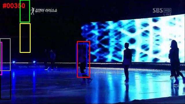
ρ and q. Setting them small will give higher influence to
more recent frames on the templates but it can lead to the
potential risk of drifting. How to set the parameters will be
discussed in section 6.1.
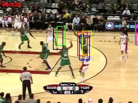
(a) davidin (b) bolt
5. Implementation Details Figure 2. Comparison of two feature selection methods based on
different loss functions. A white pixel indicates that the corre-
In this section, we discuss some implementation details sponding feature is selected, otherwise black. For each of the two
which further boost the performance of our tracker. sequences, the original image, the LASSO result and the sparse
regularized logistic regression result are shown from left to right.
5.1. Sampling Background Templates
feature selection method on these two sets separately and
In the way it was presented above, our tracker is a purely combine the two feature sets by finding their intersection.
generative model. However, when the object to track is We start with α = 0.002 and then decrease it by a factor of
heavily occluded or when it changes rapidly, the tracker 0.75 if less than half of the pixels are selected.
may not be robust enough in avoiding the drifting problem. Although a similar feature selection step is also used
To further enhance model robustness, we augment the ob- in [31], it uses the Frobenius norm for the loss (as in the
ject templates with background templates randomly sam- LASSO [22] formulation) instead of the logistic loss. We
pled from the previous frames. The dictionary templates U believe the logistic loss is a more suitable choice here since
now consist of both the original object templates Uo and the this is a classification problem. Fig. 2 shows the feature
background templates Ub . Then the weights of the particles selection results obtained by the two methods on the first
are determined by the difference in contribution
of these two frames of the davidin and bolt sequences. The logistic loss
parts, i.e., exp β(kUo Vo k1 −kUb Vb k1 ) for some param- obviously gives more discriminative features and ignores
eter β, which favors a result that can be represented well by the background area. Moreover, since the sample size n
the object templates but not by the background templates. is typically smaller than the data dimensionality (32 × 32
or 48 × 16 in our case), LASSO can never select more than
5.2. Feature Selection
n features due to its linearity. This restriction may lead to
There are two reasons why feature selection is needed. impaired performance.
First, we have assumed that raw image patches in the shape
of either rectangles or parallelograms are used to define 6. Experiments
features. However, when the tracked object has irregular
shape, the cluttered background may be included in the im- In this section, we compare the object tracking perfor-
age patch even when the tracking result is correct. Second, mance of the proposed tracker with several state-of-the-art
the tracked object may contain some variant parts which can trackers on some challenging video sequences. The trackers
incur adverse effects. Such effects should be reduced by se- compared are MTT [30], CT [27], VTD [15], MIL [3], a lat-
lecting the most invariant and informative features. So we est variant of L1T [4], TLD [13], and IVT [20]. We down-
propose using `1 -regularized logistic regression for feature loaded the implementations of these methods from the web-
selection: sites of their authors. Except for VTD, all other methods
n cannot utilize the color information in the video directly. So
o
we used the rgb2gray function in the MATLAB Image
X
log 1 + exp − li (w0 yi + b)
min + αkwk1 , (13)
w
i Processing Toolbox to convert the color video to grayscale
before performing object tracking. The code implement-
where yi is a sample from some previous frames and li is ing our method is available on the project page: http:
its corresponding label which is 1 if yi is a positive sample //winsty.net/onndl.html.
and −1 otherwise. We solve this problem using the public-
domain sparse learning package SLEP.2 Then we project the 6.1. Parameter Setting
original object templates and particles using a diagonal pro-
jection matrix P with each diagonal element pii = δ(wi ), We set λ = γ = 0.01 and η = 0.2. The parameter β
where δ(·) is the Dirac delta function. While this gives a in Sec. 5.1 is set to 5. For template update in Sec. 4.2, ρ is
more discriminative feature space for particle representa- set to 0.99 and q to 3 or 5 depending on whether the change
tion, it also reduces the computational cost. In practice, we in appearance of the tracked object is fast. The numbers
always collect negative samples from the previous frames. of object templates and background templates are set to 20
As for positive samples, besides those collected, we also use and 100, respectively. We set the template size to 32 × 32 or
the identified object from the first frame. We then run the 48×16 according to the shape of the object. The particle fil-
ter uses 600 particles. For the affine parameters in the parti-
2 http://www.public.asu.edu/ cle filter, we only select the best candidate among four pos-
˜jye02/Software/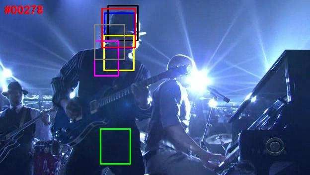
sible ones instead of performing an exhaustive grid search. Ours MTT CT VTD MIL L1T IVT
Although performing grid search may lead to better results, car4 5.3 3.4 95.4 41.5 81.8 16.8 4.2
we believe such tuning is not feasible in real environments. car11 2.3 1.3 6.0 23.9 19.3 1.3 3.2
Compared to other methods, our method is relatively insen- davidin 6.2 7.8 15.3 27.1 13.1 17.5 3.9
sitive to the values of the affine parameters. More specif- trellis 2.4 33.7 80.4 81.3 71.7 37.6 44.7
ically, our method can achieve satisfactory results in 7 out woman 7.3 257.8 109.6 133.6 123.7 138.2 111.2
of 10 video sequences when using the default parameters. bolt 7.4 35.6 12.1 22.3 9.6 237.6 7.4
The current implementation of our tracker runs at 0.7–1.5 shaking 6.7 28.1 10.9 5.2 28.6 90.8 138.4
frames per second (fps). This speed is much faster than skating1 7.2 184.0 98.2 7.4 104.4 140.4 146.9
football 6.5 15.9 12.0 6.5 14.7 27.6 17.7
the original L1T [18] and is comparable to the “realtime”
basketball 9.9 161.7 106.3 6.8 63.2 159.2 31.6
L1T [4] if the same template size and same number of par-
average 6.1 72.9 54.6 35.6 53.0 87.6 50.9
ticles are used.
Table 2. Comparison of 7 trackers on 10 video sequences in terms
6.2. Quantitative Comparison of central-pixel error (in pixels).
We use two common performance metrics for quantita- tal material. With limited space available, we try our best
tive comparison: success rate and central-pixel error. For to give a qualitative comparison by showing in Fig. 4 some
each frame, a tracker is said to be successful if the overlap key frames of each sequence.
percentage exceeds 50%. The overlap percentage is defined The car4 sequence was captured on an open road. The
area(BB T ∩BB G )
as area(BB , where BB T denotes the bounding box illumination changes greatly due to the shades of trees and
T ∪BB G )
produced by a tracker and BB G denotes the ground-truth entrance of a tunnel. All trackers except TLD do a fine job
bounding box. As for the central-pixel error, it is the Eu- before the car enters the tunnel at about frame 200. How-
clidean distance (in pixels) between the centers of BB T and ever, after that, only IVT, MTT and our tracker can track
BB G . The results are summarized in Table 1 and Table 2, the car accurately. L1T can also track it but with incorrect
respectively. For each video sequence (i.e., each row), we scale. Other methods totally fail.
show the best result in red and second best in blue. We In the car11 sequence, the tracked object is also a car but
also report the central-pixel errors frame-by-frame for each the road environment is very dark with background light.
video sequence in Fig. 3. Since TLD can report that the All methods can merely track the car in the first 200 frames.
tracked object is missing in some frames, we exclude it from However, when the car makes a turn at about frame 260,
the central-pixel error comparison. In terms of the success VTD, MIL, TLD and CT drift from the car although CT
rate, our method is always among the best two. With respect can recover later to a certain degree. Other methods can
to the central-pixel error, our method is among the best two track the car accurately.
in 8 of the 10 sequences. For the other two sequences, the The davidin sequence was recorded in an indoor envi-
gaps are quite small. We believe they can be negligible in ronment. We need to track a moving face with illumination
practical applications. and scale changes. Most trackers drift from frame 160 due
to the out-of-plane rotation. Different trackers can recover
Ours MTT CT VTD MIL L1T TLD IVT from it by various degrees.
car4 100 100 24.7 35.2 24.7 30.8 0.2 100 In the trellis sequence, we need to track the same face as
car11 100 100 70.7 65.6 68.4 100 29.8 100 in davidin but in an outdoor environment with more severe
davidin 75.5 68.6 25.3 49.4 17.7 27.3 44.4 92.0 illumination and pose changes. All trackers except MTT,
trellis 99.0 66.3 23.0 30.1 25.9 62.1 48.9 44.3 L1T and our tracker fail at about frame 160 when the person
woman 91.5 19.8 16.0 17.1 12.2 21.1 5.8 21.5 walks out of the trellis. Furthermore, L1T and MTT lose
bolt 74.7 19.5 46.2 28.3 72.7 7.5 6.8 85.7
the target at frames 310 and 350 due to the out-of-plane
shaking 98.9 12.3 92.3 99.2 26.0 0.5 15.6 1.1
skating1 92.5 9.5 3.8 93.3 6.8 5.3 47.0 6.5
rotation. TLD is unstable in getting and losing the target
football 82.9 70.7 69.6 80.4 76.2 30.7 74.9 56.3 several times. On the other hand, our tracker can track the
basketball 97.2 14.8 24.6 98.6 32.3 7.4 2.3 17.1 face accurately along the whole sequence.
average 91.2 48.2 39.6 59.7 36.3 35.8 29.3 52.5 In the woman sequence, we track a walking woman in
the street. The difficulty lies in that the woman is greatly
Table 1. Comparison of 8 trackers on 10 video sequences in terms
occluded by the parked cars. TLD fails at frame 63 because
of success rate (in percentage).
the pose of the woman changes. All other trackers com-
pared fail when the woman walks close to the car at about
6.3. Qualitative Comparison frame 130. Our tracker can follow the target accurately.
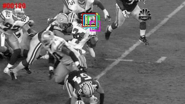
In the bolt sequence, the target is a running athlete with
Complete video sequences with the bounding boxes re-
rapid changes in appearance. L1T and MTT fail at some in-
ported by different trackers are provided in the supplemen-
car4 car11 davidin trellis woman
250 100 150 250 800
200 80 200
600
Center Error
Center Error
Center Error
Center Error
Center Error
100
150 60 150
400
100 40 100
50
200
50 20 50
0 0 0 0 0
0 200 400 600 800 0 100 200 300 400 0 100 200 300 400 500 0 200 400 600 0 200 400 600
Frame Number Frame Number Frame Number Frame Number Frame Number
bolt shaking skating1 football basketball
500 300 400 100 800
400 250 80
300 600
Center Error
Center Error
Center Error
Center Error
Center Error
200
300 60
150 200 400
200 40
100
100 200
100 50 20
0 0 0 0 0
0 100 200 300 0 100 200 300 400 0 100 200 300 400 0 100 200 300 400 0 200 400 600 800
Frame Number Frame Number Frame Number Frame Number Frame Number
Ours IVT CT MIL L1T VTD MTT
Figure 3. Frame-by-frame comparison of 7 trackers on 10 video sequences in terms of central-pixel error (in pixels).
termediate frames, but all other trackers can track the target efficient multiplicative update rule. It can be further shown
successfully till the end. Among all methods, ours and IVT that our new formulation is equivalent to the approach of us-
get the most accurate result. ing trivial templates by other sparse trackers. We have con-
In the shaking sequence, the tracked head is subject to ducted extensive comparative studies on some challenging
drastic pose and illumination changes. L1T, IVT and TLD benchmark video sequences and shown that our proposed
totally fail before frame 10, while MTT and MIL show tracker generally outperforms existing methods.
some drifting effects then. VTD gives the best result, which One possible extension of our current method is to ex-
is followed by our tracker and CT. ploit the underlying structures and relationships between
The skating1 sequence contains abrupt motion, occlu- particles, as in MTT [30]. We expect it to lead to further
sion and significant illumination changes, which make most performance gain.
trackers fail. Our tracker gives comparable result with VTD. Acknowledgment
The football sequence aims to track a helmet in a football
match. The difficulty lies in that many helmets are similar This research has been supported by General Research Fund
621310 from the Research Grants Council of Hong Kong.
in background. Moreover, collision with another player of-
ten confuses most trackers. Only our tracker and VTD can References
successfully locate the correct object.
[1] M. Aharon, M. Elad, and A. Bruckstein. K-SVD: An al-
In the basketball sequence, the appearance of the tracked
gorithm for designing overcomplete dictionaries for sparse
player changes rapidly in the intense match. Moreover, the representation. IEEE Transactions on Signal Processing,
players in the same team have similar appearance. Only 54(11):4311– 4322, 2006. 2
VTD and our tracker can survive to the end. [2] M. Arulampalam, S. Maskell, N. Gordon, and T. Clapp. A
We note that the football and basketball sequences tutorial on particle filters for online nonlinear/non-Gaussian
demonstrate the effectiveness of sampling background tem- Bayesian tracking. IEEE Transactions on Signal Processing,
plates as described in Sec. 5.1. It helps a lot in distinguish- 50(2):174–188, 2002. 3
ing the true target from distractors in the background. [3] B. Babenko, M.-H. Yang, and S. Belongie. Robust ob-
ject tracking with online multiple instance learning. IEEE
Transactions on Pattern Analysis and Machine Intelligence,
7. Conclusion and Future Work 33(8):1619–1632, 2011. 2, 5
[4] C. Bao, Y. Wu, H. Ling, and H. Ji. Real time robust L1
In this paper, we have proposed a novel visual tracking
tracker using accelerated proximal gradient approach. In
method based on robust non-negative dictionary learning.
CVPR, pages 1830–1837, 2012. 2, 5, 6
Instead of taking an ad hoc approach to update object tem-
[5] A. Doucet, D. N. Freitas, and N. Gordon. Sequential Monte
plates, we formulate this procedure as a robust non-negative Carlo Methods In Practice. Springer, New York, 2001. 1, 2
dictionary learning problem and propose a novel online pro- [6] L. Du, X. Li, and Y.-D. Shen. Robust nonnegative matrix fac-
jected gradient descent method to solve it. The most ap- torization via half-quadratic minimization. In ICDM, pages
pealing advantage is that it can detect and reject the occlu- 201–210, 2012. 2
sion and cluttered background automatically. Besides, we [7] H. Grabner, M. Grabner, and H. Bischof. Real-time tracking
have proposed to get rid of the trivial templates by using via on-line boosting. In BMVC, pages 47–56, 2006. 2
the Huber loss function in particle representation. To solve [8] S. Hare, A. Saffari, and P. H. Torr. Struck: Structured output
the resulted optimization problem, we devise a simple and tracking with kernels. In ICCV, pages 263–270, 2011. 2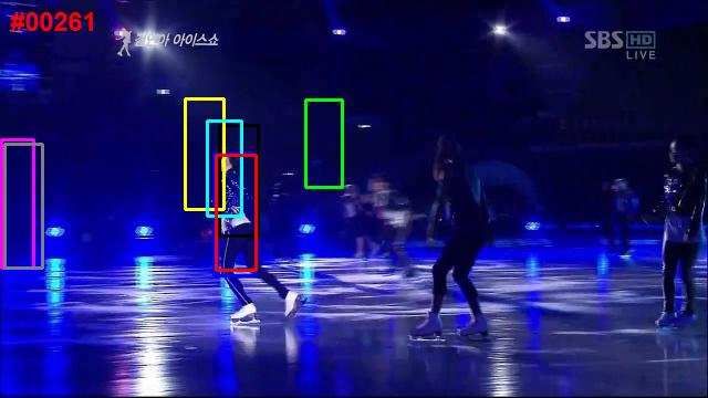
(b)car11
     (a)car4
    (c)davidin

                                                                             (d)trellis
                                                                          (f)basketball
     (e)woman

                                                                          (j)football (h)shaking
     (i)skating1 (g)bolt

                                              Ours    IVT    CT     MIL                  L1T        TLD    VTD     MTT

                           Figure 4. Comparison of 8 trackers on 10 video sequences in terms of bounding box reported.

 [9] P. Hoyer. Non-negative sparse coding. In Proceedings of the                             [21] D. Seung and L. Lee. Algorithms for non-negative matrix
     Workshop on Neural Networks for Signal Processing, pages                                     factorization. NIPS, pages 556–562, 2001. 2
     557–565, 2002. 2                                                                        [22] R. Tibshirani. Regression shrinkage and selection via the
[10] P. Huber. Robust estimation of a location parameter. The                                     lasso. Journal of the Royal Statistical Society. Series B
     Annals of Mathematical Statistics, 35(1):73–101, 1964. 1, 3                                  (Methodological), 58(1):267–288, 1996. 1, 5
[11] X. Jia, H. Lu, and M.-H. Yang. Visual tracking via adaptive                             [23] N. Wang, T. Yao, J. Wang, and D.-Y. Yeung. A probabilis-
     structural local sparse appearance model. In CVPR, pages                                     tic approach to robust matrix factorization. In ECCV, pages
     1822–1829, 2012. 2                                                                           126–139, 2012. 2, 4
[12] Z. Kalal, J. Matas, and K. Mikolajczyk. P-N learning:                                   [24] Y. Wu, J. Lim, and M.-H. Yang. Online object tracking: A
     Bootstrapping binary classifiers by structural constraints. In                               benchmark. In CVPR, 2013. 2
     CVPR, pages 49–56, 2010. 2                                                              [25] J. Yang, K. Yu, Y. Gong, and T. Huang. Linear spatial pyra-
[13] Z. Kalal, K. Mikolajczyk, and J. Matas. Tracking-learning-                                   mid matching using sparse coding for image classification.
     detection. IEEE Transactions on Pattern Analysis and Ma-                                     In CVPR, pages 1794–1801, 2009. 2
     chine Intelligence, 34(7):1409–1422, 2012. 2, 5                                         [26] A. Yilmaz, O. Javed, and M. Shah. Object tracking: A sur-
[14] D. Kong, C. Ding, and H. Huang. Robust nonnegative ma-                                       vey. ACM Computing Surveys, 38(4), 2006. 2
     trix factorization using L21-norm. In CIKM, pages 673–682,                              [27] K. Zhang, L. Zhang, and M.-H. Yang. Real-time compres-
     2011. 2                                                                                      sive tracking. In ECCV, pages 864–877, 2012. 2, 5
[15] J. Kwon and K. Lee. Visual tracking decomposition. In
                                                                                             [28] S. Zhang, H. Yao, X. Sun, and X. Lu. Sparse coding based
     CVPR, pages 1269–1276, 2010. 2, 5
                                                                                                  visual tracking: review and experimental comparison. Pat-
[16] C. Lu, J. Shi, and J. Jia. Online robust dictionary learning.                                tern Recognition, 46(7):1772–1788, 2012. 2
     In CVPR, 2013. 2, 4
                                                                                             [29] T. Zhang, B. Ghanem, S. Liu, and N. Ahuja. Low-rank sparse
[17] J. Mairal, F. Bach, J. Ponce, and G. Sapiro. Online learn-
                                                                                                  learning for robust visual tracking. ECCV, pages 470–484,
     ing for matrix factorization and sparse coding. Journal of
                                                                                                  2012. 1, 2
     Machine Learning Research, 11(1):19–60, 2010. 2, 4
                                                                                             [30] T. Zhang, B. Ghanem, S. Liu, and N. Ahuja. Robust vi-
[18] X. Mei and H. Ling. Robust visual tracking using l1 mini-
                                                                                                  sual tracking via multi-task sparse learning. In CVPR, pages
     mization. In ICCV, pages 1436–1443, 2009. 1, 2, 6
                                                                                                  2042–2049, 2012. 1, 2, 5, 7
[19] X. Mei, H. Ling, Y. Wu, E. Blasch, and L. Bai. Minimum
                                                                                             [31] W. Zhong, H. Lu, and M.-H. Yang. Robust object track-
     error bounded efficient l1 tracker with occlusion detection.
                                                                                                  ing via sparsity-based collaborative model. In CVPR, pages
     In CVPR, pages 1257–1264, 2011. 2
                                                                                                  1838–1845, 2012. 2, 5
[20] D. Ross, J. Lim, R. Lin, and M. Yang. Incremental learning
     for robust visual tracking. International Journal of Computer
     Vision, 77(1):125–141, 2008. 2, 4, 5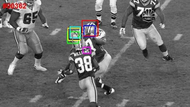
You can also read