Senseable City Lab : Massachusetts Institute of Technology
←
→
Page content transcription
If your browser does not render page correctly, please read the page content below
Senseable City Lab :.:: Massachusetts Institute of Technology
      This paper might be a pre-copy-editing or a post-print
  author-produced .pdf of an article accepted for publication. For
    the definitive publisher-authenticated version, please refer
           directly to publishing house’s archive system

                            SENSEABLE CITY LAB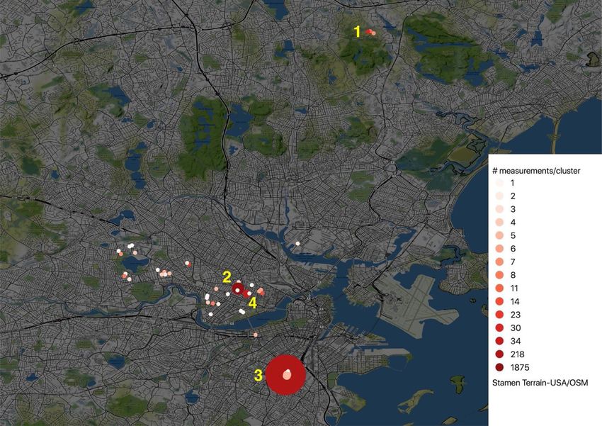
Sustainable Cities and Society 60 (2020) 102239

                                                                      Contents lists available at ScienceDirect

                                                             Sustainable Cities and Society
                                                           journal homepage: www.elsevier.com/locate/scs

Air quality monitoring using mobile low-cost sensors mounted on trash-                                                                                                   T
trucks: Methods development and lessons learned
Priyanka deSouzaa,*, Amin Anjomshoaaa, Fabio Duartea,b, Ralph Kahnc, Prashant Kumard,
Carlo Rattia
a
  Senseable City Lab, Massachusetts Institute of Technology, Cambridge MA, United States
b
  Pontifícia Universidade Católica do Paraná, Brazil
c
  NASA Goddard Space Flight Center, Greenbelt, MA, 20771, United States
d
  Global Centre for Clean Air Research (GCARE), Department of Civil and Environmental Engineering, Faculty of Engineering and Physical Sciences, University of Surrey,
Guildford, GU2 7XH, United Kingdom

A R T I C LE I N FO                                         A B S T R A C T

Keywords:                                                   Air quality monitoring (AQM) is crucial for cities to develop management plans supporting population health.
Drive-by sensing                                            However, there is a dearth of measurements due to the high cost of standard reference instruments. Mobile AQM
Low-cost sensors                                            using low-cost sensors deployed on routine fleets of vehicles can enable the continuous detection of fine-scale
Particulate matter                                          pollutant variations in cities at a lower cost. New methods need to be developed to interpret these measure-
Routine sampling
                                                            ments. This paper presents three such methods. First, we propose a technique to identify aerosol hotspots.
                                                            Second, we employ techniques published previously to assess the generalizable map of fine and coarse particle
                                                            number concentrations, to understand qualitatively the contribution of local and regional sources across the
                                                            region sampled. By using the raw number concentration of differently sized particles from the Optical Particle
                                                            Counters (OPCs) instead of the noisier mass concentrations, we obtain more robust results. Third, in order to
                                                            evaluate source signatures in cities, we propose another technique, in which we cluster the entire range of
                                                            aerosol size-distribution measurements acquired. The properties of each cluster provide insight into the aerosol
                                                            source characteristics in the sampling environment. We test these methods using a dataset we collected by
                                                            mounting OPCs on two trash-trucks in Cambridge, Massachusetts.

1. Introduction                                                                                       The difficulty of working with mobile air quality monitoring data
                                                                                                  arises from the combination of complex spatiotemporal sampling and
    Poor air quality is a major environmental health risk in cities. Air                          temporal air quality variability in different locations, related to traffic
quality monitoring is crucial for developing informed air quality man-                            dynamics, street topology, meteorology, background source strength,
agement plans. However, setting up and maintaining air quality                                    etc. (Goel & Kumar, 2015; Van den Bossche et al., 2015). As mobile
monitors is expensive. Even in the United States, resource constraints                            sensors capture only a snapshot of air pollution at a given location and
dictate that the regulatory air quality monitoring network is sparse,                             time, this temporal variability makes it difficult to characterize the air
with only 2–5 regulatory monitors per 1 million people or 1000 km2 in                             pollution at a given location based on these measurements alone. In
60 % of US census urban areas (Apte et al., 2017).                                                order to produce detailed, representative aggregate air quality maps,
    Furthermore, air pollutant concentrations in complex urban en-                                large amounts of data over different meteorological and traffic condi-
vironments display high variability and sharp gradients over distances                            tions would be required (Apte et al., 2017; Brantley et al., 2013).
as small as 10 m (Brantley et al., 2013; Van den Bossche et al., 2015).                               ‘Purpose-built’ mobile air quality monitoring labs often require
To characterize the reactive-pollutant spatial variation in situ, even a                          dedicated vehicles and trained research staff as drivers. For this reason,
dense (but realistic) network of fixed air quality monitors cannot cap-                            most mobile air quality monitoring studies to date have been relatively
ture this variability. Mobile air quality monitoring can be used to obtain                        short-term campaigns and provide insufficient repetitive frequency to
air pollution concentrations at high spatial resolution with a smaller                            reveal long-term spatial air quality trends in a city (Bukowiecki et al.,
number of monitors over a fixed period of time.                                                    2002; Kolb et al., 2004; Pirjola et al., 2012, 2004). Apte et al. (2017)

    ⁎
        Corresponding author.
        E-mail address: desouzap@mit.edu (P. deSouza).

https://doi.org/10.1016/j.scs.2020.102239
Received 29 September 2019; Received in revised form 10 May 2020; Accepted 11 May 2020
Available online 18 May 2020
2210-6707/ © 2020 Elsevier Ltd. All rights reserved.
P. deSouza, et al.                                                                                                         Sustainable Cities and Society 60 (2020) 102239

conducted one of the first long-term mobile air quality monitoring                       dN
                                                                                              per volume of air at Dmidpoint =
                                                                                                                                            ΔN
studies with a routine fleet of vehicles. Their study used high-quality                dln (D)                                   ln (Dupper ) − ln (Dlower )
reference PM air quality monitors on Google Street View cars to re-                                                                  1
                                                                                                                    ×
peatedly sample every street in Oakland, CA, over the course of a year.                                                 flow rate × sampling time                     (1)
    On the other end of the spectrum of air quality monitors, the use of
low-cost monitors (costing less than USD $3000) is increasing (Kumar                      where N is the number concentration of PM within a size bin
et al., 2015; Morawska et al., 2018; Snyder et al., 2013), and several                (#/mL), D is the diameter of the particles, Dupper, Dlower and Dmidpoint
community-based mobile monitoring studies have used these low-cost                    are the upper, lower and midpoint diameters of the OPC-N2 bins in
instruments (Dutta et al., 2009; Elen et al., 2013). Mahajan and Kumar                units of (μm), ΔN is the number of particle-counts in each bin.
(2020) have evaluated the use of low-cost sensors for quantifying per-                    The particle counts agree well with reference instrument measure-
sonal exposure. Low-cost monitors offer the possibility of systematic air              ments for coarser particles (> 0.78 μm), providing detection efficiency
quality monitoring even for resource-limited cities.                                  ranging from 83 %–108 %, but the particle counts for finer particles
    We add to this literature by developing new techniques to analyse                 (< 0.78 μm) are underestimated (detection efficiency ∼78 % for mono-
measurements from mobile low-cost sensors deployed on another rou-                    disperse polystyrene spheres (Sousan, Koehler, Hallett, & Peters, 2016).
tine fleet of vehicles: trash-trucks, which are deployed in nearly all                 Despite the greater noise in the detection of particles in the lower bins,
major cities globally. Specifically, we show how data from mobile, low-                the OPC measurements still provide useful information of the amount of
cost sensors can be used: 1) to detect pollution hot spots from major,                finer aerosol in the atmosphere, and we retain these bins in this ana-
fixed, possibly intermittent sources in the built environment, 2) to de-               lysis.
velop a qualitative understanding of where local versus regional sources                  A partly proprietary Alphasense data reduction algorithm makes
dominate in a city, and 3) to identify pollutant source signatures on                 assumptions about particle density and the number of particles with
different street segments. Such insights about air pollution can help city             diameters smaller than 0.38 μm, to report PM1, PM2.5 and PM10. These
managers develop effective air quality management plans.                               assumptions create uncertainty in the PM values that vary based on the
    Anjomshoaa et al. (2018) compared the utility scheduled vehicles,                 ambient aerosol size distribution and density at the time of measure-
such as trash-trucks, with non-scheduled vehicles, such as taxis, as                  ment.
urban air quality sensing platforms in cities. Although taxis operate                     Although the Alphasense OPC-N2 monitors are thus of lower quality
24 h a day and potentially sample at a higher rate the busiest streets in a           than reference instruments, the particle number concentration mea-
city, there is no guarantee that they cover all streets. On the other hand,           surements in 16 size bins represent much better constraints on the true
although trash-trucks operate for short periods during the day, and                   values than the derived, size-resolved particle mass, as exemplified by
have a lower sampling frequency of most streets, they provide complete                the work of Sousan et al. (2016). Such information can constrain the
spatial coverage of city streets. Therefore, using trash-trucks as a scal-            aerosol size distribution over space, which can indicate local/regional
able sampling platform is worth investigating.                                        pollution sources, as we demonstrate in the current study. It must be
    We test our techniques using measurements made in Cambridge,                      noted that If the aerosol is hygroscopic, under conditions of high hu-
Massachusetts, between April 21, 2017 and August 14, 2017, where we                   midity (RH > 85 %) the OPC interprets the hydrated particles as larger
deployed low-cost Optical Particle Counters (OPC-N2s) on two trash-                   “dry” particles, and the reported number concentrations will have er-
trucks as a pilot experiment.                                                         rors (Crilley et al., 2018). The RH during times of measurement in
    The rest of this paper is organized as follows: Section 2 describes the           Cambridge was between 60–70 %, and therefore particle hydration is
data used, the collection strategy, and the analysis methods. Section 3               unlikely to be a major concern during our experiment.
presents the results obtained from applying the three methods sketched                    In addition to characterizing the variation of PM1, PM2.5 and PM10
out above to our Cambridge dataset. Lessons learned and practical                     across our sampling route, we also aggregate the spatial variation of
implications for future deployments are given in Section 4.                           particle number concentrations in different size bins derived from the
                                                                                      raw OPC-N2 measurements: N1 (N0.38-1, comprising particles with
                                                                                      diameters between 0.38 μm and 1 μm), and coarser particles: N12 (N1-
2. Materials                                                                          12, covering particles with diameters between 1 μm and 12 μm).
                                                                                          For more information about the experiment design, the study area
2.1. Low-cost particulate matter monitors                                             and sampling protocol and the days on which sampling runs occurred in
                                                                                      Cambridge, MA, please refer to Section S1 in Supplementary
    We use the data collected by Alphasense OPC-N2 monitors1 de-                      Information.
ployed on two trash-trucks in the City of Cambridge for a total of 27
days between April and August 2019, to gain qualitative insights into                 3. Methods
potential sources of PM in this urban environment. The Alphasense
OPC-N2 sensor measures particle counts (N0.38-17.5) in 16 size bins                      In this section we present three techniques designed to identify and
ranging from 0.38 to 17.5 μm (Table S1, Supplementary Information).                   characterize PM2.5 hotspots, to estimate the generalised air pollution
The OPC works by illuminating one particle at a time with focused laser               over the sampled routes, and to analyze aerosol size distribution from
light and measuring the intensity of light scattered. The amount of                   the OPC-N2s, yielding estimates of PM source signatures in different
scattering from a particle is a function of the particle size. The instru-            parts of the sampling route.
ment is calibrated using monodisperse particles of known size to derive
counts for particles of different sizes.                                               3.1. Identification and characterization of PM2.5 hotspots
    The number and volume concentrations of particles can be obtained
by dividing the particle counts by the flow rate and sampling time. The                    We identified all measurements where PM2.5 > 100 μg/m3, that we
log-normal size distribution of particles at the midpoint of each dia-                arbitrarily selected to be much higher than the EPA daily average
meter bin can be calculated using Eq. (1):                                            standard of 35 μg/m3. Such high measurements are substantially above
                                                                                      the background values in the study region, as presented subsequently,
                                                                                      and could either be 1) noise from the OPC-N2, or 2) an indicator of a
                                                                                      strong local source of pollution.
     1
         http://www.alphasense.com/index.php/products/optical-particle-counter/           In order to identify measurements that were products of local
”.                                                                                    sources rather than noise, we used hierarchical clustering (Johnson,

                                                                                  2
P. deSouza, et al.                                                                                                  Sustainable Cities and Society 60 (2020) 102239

1967; Langfelder & Horvath, 2012) to cluster measurements made in                approach to be an effective way to account for background con-
the same spatial area using a distance cut off of 100 m.                          centrations for a range of pollutants in their North Carolina study over a
    We calculated the number of measurements in each cluster, as well            variety of meteorological conditions and sampling routes.
as the number of unique days over which the measurements in each                     Once the method for evaluating background air pollution was se-
cluster were made. Most clusters contained only a few measurements,              lected, we performed a background time-of-day correction using
indicating that they could represent measurement noise. We thus only             Equations 2 and 3 to account for the period during which the trucks
focused on clusters that contained > 30 measurements, or those for               operated:
which the number of unique measurement days was greater than 1. We
                                                                                 PM2.5,norm i= PM2.5,OPC, i x PM2.5,   bkg,median   / PM2.5,bkg,i              (2)
characterized each cluster by calculating the average properties (PM1,
PM2.5, PM10, N1, N12) of each cluster. The temporal nature of these              where PM2.5,OPC,i is the OPC measurement for event i, PM2.5,bkg, i is the
hotspots and their average properties allow us to deduce potentially             contemporaneous background value of pollution over the entire region,
important local fixed sources that contribute to the hotspot formation.           and PM2.5, bkg,median is the median of the PM2.5,bkg values on the day of
This information is useful for planners in developing air pollution              measurement for the time period 07:00 to 14:00 h (local time).
management plans.                                                                    However, Cambridge is a city with relatively clean air, so the
    Even in locations where we see pollution hotspots, it is possible that       background PM2.5 is often very low. As a result, we apply an additive
the source involved only operates for short periods of time, so typical          rather than a multiplicative background-correction factor:
pollutant concentrations might be low. In the next subsection, we de-
scribe how we obtain the relative distribution of typical pollutant              PM2.5,norm i= PM2.5,OPC i - PM2.5,   bkg,i   + PM2.5,   bkg,median            (3)
concentrations across the trash-truck sampling route.                               By subtracting the time-of-day-resolved regional background from
                                                                                 the pollution measurement, we can now compare local air pollution
3.2. Methodology for estimating generalized air pollution over the sampled       over space. Note that, conversely, PM2.5 in Equations 2 and 3 can be
routes                                                                           replaced with particle number concentrations (N1 or N12) to estimate
                                                                                 background-corrected aerosol number concentrations.
3.2.1. Pre-processing: background correction
    To compare measurements made at the same location but on dif-
ferent days and at different times, we need to account for possible bias          3.2.2. Estimating generalizable pollutant values across the sampling route
created by diurnal variation in background aerosol number con-                       Given our large dataset (> 500,000 observations), we applied a
centration and PM concentrations over the study region. We assume                series of steps to convert the data into estimates of median concentra-
that the background value varies temporally but not spatially over the           tions for individual road segments over all sampling runs. We con-
region.                                                                          structed these road segment estimates by dividing the Cambridge street
    We assessed the background contribution using three different                 network into segments of fixed lengths, using the ‘Locate Points Along
methods. The first method involves applying an hourly multiplicative              Lines’ QGIS Python Plugin (https://plugins.qgis.org/plugins/
factor derived from concentrations reported by a reference air quality           LocatePoints/). We adopted a process for aggregating these data and
monitor at a designated background site (Hagler et al., 2012; Van                deriving sampling error from previous work (e.g., Apte et al. (2017)).
Poppel, Peters, & Bleux, 2013). In our case, this requires using the                 First, we spatially-aggregated all our mobile (1) background-ad-
regulatory monitor at Boston’s North End (N:42.363, E:-71.055, 4 km              justed PM2.5, and (2) background-adjusted number-concentration
southeast of the center of the study region). Unfortunately, here is no          measurements for 0.38 μm–17.5 μm particles from the OPC-N2s, by
reference air quality monitor in Cambridge, the site of our experiment.          snapping them to the road segment on which they were acquired. This
This technique involves uncertainties, in part because the OPC optical           allows measurements made in the same segment to be analysed as a
measurements are not directly comparable to the reference monitor’s              group. This distance is small enough to capture pollutant-concentration
gravimetric ones.                                                                gradients, but is not so finely sliced that GPS errors overwhelm the
    The second method, following (Bukowiecki et al., 2002), takes the            results. Therefore, we also use segment lengths of 30 m.
lowest 10th percentile of the pollutant concentrations for a given hour              Second, we selected the median as an outlier-resistant metric of PM
during the run as the fixed background value for that run.                        and number concentration central tendency, as others have done (Apte
    The third method uses a time-series, spline-of-minimums approach,            et al., 2017; Hankey & Marshall, 2015). We chose not to remove peak
presented by Brantley et al. (2013), to estimate the background number           concentrations caused by encounters with vehicle exhaust plumes, as
concentrations of finer particles: N1, N12, as well as PM2.5 for each day.        such plumes contribute to the particle concentration at a given location.
We did this by (a) applying a rolling 30-second mean to smooth the               For comparison, we also calculated the mean values, with the under-
measurements, (b) dividing the time series into discrete 10-minute               standing that individual outliers can significantly skew those results.
segments and locating the minimum concentration in each segment,                     Third, we used a set of bootstrap resampling procedures to quantify
and (c) fitting a smooth, thin-plate regression spline through the                the effect of sample-to-sample variability and of sampling error on the
minimum concentrations. Note that on nine days the two OPCs were                 median concentrations. As a metric of precision, we used the ratio of
operating simultaneously. We consider the total observations made for            standard error of the median (mean) concentration to the median
a given day in this methodology, consistent with our assumption that             (mean) concentration itself. In general, the average skew of the median
the background is temporally varying but spatially uniform.                      PM2.5 concentrations for the 30 m segments is ∼0.9. This indicates that
    We compared each of the three proposed methods to choose a                   the distributions are close to central tendency, with the mean slightly
background pollution value, and found that they produced similar                 greater than the median.
corrected values. Specifically, the mean differences in the corrected N1,
N12 and PM2.5 values using the different methods were less than 5%.               3.3. Working with the aerosol size distribution from the OPC-N2s
The differences between the corrected values and the raw N1, N12 and
PM2.5 measurements were also less than 5% (Table S2 in                               It is challenging to analyse the aerosol size distribution at each point
Supplementary Information). Given the minimal differences in back-                in time, because for each measurement Eq. (1) allows us to calculate the
ground-corrected number concentrations and PM2.5 values vis a vis the            size distribution at the midpoint of each of the 16 bins. We thus have 16
raw measurements using the different methods, we chose the splines-of-            data points for each time-step. Pey et al. (2008) showed that aerosol
minimum approach to obtain background concentrations for all pollu-              number and mass concentrations can be affected by multiple sources
tants. This is supported by Brantley et al. (2013), who found this               and atmospheric processes.

                                                                             3
P. deSouza, et al. Sustainable Cities and Society 60 (2020) 102239
To simplify the analysis of the OPC size distributions systematically, zone. (See Fig. S2 in Supplemental Information, which displays the
we clustered the size-bin observations (without background-correction) number of unique days over which each street along the trash-truck
using the k-means technique. The final cluster centres reflect particle routes was sampled.)
number size distributions representative of each cluster, thereby redu- 2) The location of cluster 2 is at the Department of Public Works,
cing the complexity of the dataset (Beddows, Dall’Osto, & Harrison, where the trash-trucks are housed. This is the largest hotspot,
2009). This technique allows us to identify a small number of typical with > 1,800 PM2.5 measurements exceeding 100 μg/m3. Although
aerosol size distributions that can be compared across space and time, the trash-trucks travelled to and from this location on every day of
which can give us insights into the kinds of sources responsible for their operation, such high PM2.5 values were seen on only three days
measurements within a cluster. during the experiment.
Without access to the size distribution of the background aerosol, it 3) The third cluster is located at a waste collection site in Roxbury,
is impossible to perform a background correction on the aerosol size Boston, MA. The number of unique days over which measurements
distribution. However, by applying the k-means clustering technique on comprising this cluster were made is ten. This indicates that there is
the complete range of raw size distribution data, we are able to gain a likely a major, fairly consistent source of particulate matter at this
better understanding of the source attribution of aerosols in the sam- site.
pling route environment. 4) The last PM2.5 cluster is on Hamlin Street, in Cambridge, close to a
In order to choose the number of clusters, we examined the within- large parking area and a park. It consists of 34 measurements made
group sum-of-squares error for cluster sizes ranging from 2 to 30 to over a span of two unique days.
determine an optimum number of clusters. Fig. S3 in Supplementary
Information shows that the error in representing the full dataset de- The modal diameter of the aerosol distribution on Hamlin Street and
creases sharply between 1 and 4 or 5 clusters. When we applied k- one of the clusters at Saugus (the smaller cluster, comprising 11 mea-
means clustering with more than 5 groups, the average size distribu- surements) is > 1 μm, as seen in Table associated with Fig. S4. As most
tions of the newly created clusters had a similar shape to that of pre- combustion pollution particles tend to be well below 0.5 μm in dia-
viously identified clusters, albeit with different total number con- meter, this suggests that local soil or dust particles make a large con-
centrations. Normalizing the size distribution by the number tribution to pollution at these sites. From the Table associated with Fig.
concentration of aerosols per measurement might have led to better S4, the high ratios of PM10/PM2.5 for these clusters bolsters this hy-
results. Unfortunately, because the OPC doesn’t detect particles with pothesis. The shape of the average aerosol size distribution of the other
diameters < 0.38 μm, the total aerosol number concentration at each cluster at Saugus indicates a massive number concentration of fine
measurement is unknown, and we were thus unable to normalize the particles at this site, which is borne out by the low PM10/PM2.5, high N1
measured size distribution. and low N12 concentrations. At Roxbury, the shape of the aerosol
To avoid over-interpreting the data, we cluster the data into five distribution indicates a complex environment, with high concentrations
groups. We evaluated the average size distribution and the spatial and of fine as well as coarser particles. A massive number concentration of
temporal variation of each cluster to infer source characteristics and coarse particles is found at the Cambridge Public Works Department.
assess the aerosol dynamics at work in our dataset. Three of the four hotspot locations identified above are at waste
disposal sites, and the Cambridge Public Works Department con-
4. Results and Discussion of the application of these techniques in centration is likely due to the indoor housing of trash-trucks. In both
Cambridge cases, it indicates that personnel, such as the trash-truck drivers, are
exposed to high pollution values at these locations. Stationary mon-
4.1. Hotspot identification itoring would be required to measure air quality at the sites when the
trash-trucks are not present, to interpret these air pollution values
Fig. 1 shows the results of performing hierarchical clustering on generally.
PM2.5 measurements > 100 μg/m3 as described in Section 3.1. Forty- In the next subsection, we highlight the general values of pollution
four distinct clusters were identified. Thirty-seven of the clusters con- across the sampling routes, taking into consideration all measurements
tained fewer than 10 measurements made over the course of a unique made over the period of study. This gives us information about the
day, indicating that these spikes could be artefacts. We highlight in ‘typical’ sources that contribute to pollution at each location.
Fig. 1 four of the seven other clusters of PM2.5 values recorded by the
OPC, where the number of measurements is > 30, or the number of 4.2. Spatial patterns
unique days over which the measurements are made are > 1.
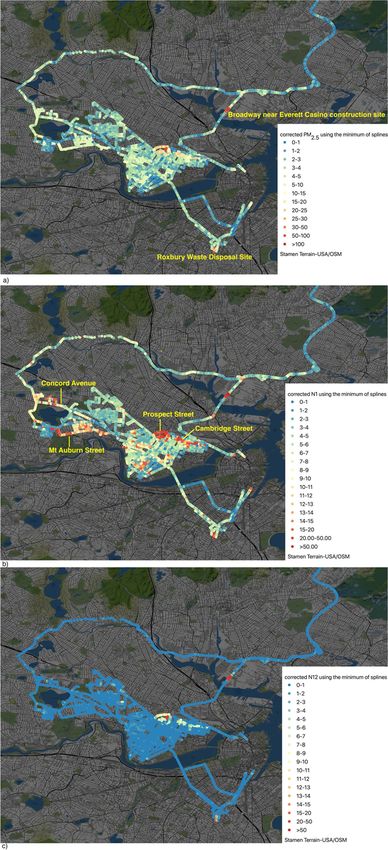
Table S3 in Supplementary Information reports the number of The median background-corrected concentration of PM2.5, fine
measurements that comprise each cluster and the number of unique particles (N1), and coarse particles (N12) are depicted in Fig. 2a, b and
days over which measurements in each cluster were made. Table S3 c respectively. Fig. S5a (Supplementary Information) shows the median
also provides a google maps image of the location at which each cluster PM2.5 on road segments where the normalised error in the median
was made. All of these clusters were only detected on a handful of days, PM2.5 derived from bootstrapping is ≤20 %, and the number of unique
indicating the temporal intermittency of the local sources responsible days on which a road segment was sampled exceeds unity. Fig. S5b and
for these hotspots that we now explore. In addition, Fig. S4 in the c are similar plots for N1, and N12. Fig. S5 thus shows us pollutant
Supplementary Information depicts the average particle size distribu- values at locations along the sampling route for which we are reason-
tion for each cluster. The Table associated with Fig. S4 reports the ably confident to have estimated the ‘typical’ value of pollution during
average PM1, PM2.5, N1, N12 for each cluster and the time at which the the period of study.
measurements in each cluster were observed. Fig. 2a indicates that on average, PM2.5 in Cambridge is likely low
We now explore each of the four robust hotspots in detail: and uniform across the city for weekdays between 07:00 to 14:00 local
time, when and where the trash-trucks operate. Some of the locations
1) Cluster 1 comprises 30 measurements of high PM2.5 values that were where high PM2.5 values are observed coincide with previously iden-
made at the site marked ‘1’ in Fig. 1, which is an organic farm in tified hotspots, such as at the Roxbury waste disposal/transfer site,
Rocky Hill Farm, in the city of Saugus, Massachusetts, also a site of whereas at the Cambridge Public Depot and Hamlin Street, we see
waste disposal. A smaller cluster comprising 11 measurements is PM2.5 observed are only moderately high, indicating that hotspots of
nearby. However, it is worth noting that on only one of the 27 days pollution in the latter locations are sporadic or atypical.
of sampling a trash-truck travelled north to the Saugus dumping High values of PM2.5 over the period of study were also observed on
4P. deSouza, et al. Sustainable Cities and Society 60 (2020) 102239
Fig. 1. Locations of the centroid of clusters produced via hierarchical clustering described in Section 3.1. The color of the cluster represents the number of data points
in each cluster. The size of the cluster corresponds to the number of unique days of measurement corresponding to each cluster. Four large hotspots/clusters (number
of points in the cluster are > 10 and number of unique days of measurement > 1) are identified and numbered.
Prospect Street (close to the trash-truck depot), as well as on Broadway 4.3. Analysis of the size distribution of particulates monitored
across the Malden Bridge, near the Everett Casino construction site. As
the normalised error in the median is > 20 % (Fig. S5a), further gen- As discussed in Section 3.3, we used K-means clustering to interpret
eralizable statements about levels of pollution at these locations would the OPC particle size-concentration data, and identified five clusters in
require more measurements. The sites with the highest PM2.5 values in the optimal grouping. Unlike the hierarchical clustering method pre-
Fig. 2a also appear as hot spots for N1 (Fig. 2b) and N12 (Fig. 2c), sented in Section 3.1, where similar measurements located within a
indicating high concentrations of both sub-micron and super-micron radius of 100 m of each other were grouped, we use the k-means ana-
particles. However, from Fig. S5b and c, as for PM2.5, only the calcu- lysis to identify signatures of similar sources across time and space. The
lated ‘generalizable’ N1 and N12 concentrations at the Roxbury waste average size distribution of each cluster is shown in Fig. 3. Table 1 gives
transfer/disposal site is stable. More measurements need to be made at the average pollutant concentrations and trash-truck velocity corre-
the other locations to gain confidence in the ‘typical’ pollutant con- sponding to each cluster, as well as the number of days on which
centration levels at these locations. Other than these sites, the PM2.5 measurements corresponding to each cluster were made.
values observed during the sampling are much lower than the EPA daily Fig. 3 shows that the aerosol concentration mode values for clusters
averaged standard of 35 μg/m3 overall, as well as the EPA annual 3 and 5 occur at ∼0.78 μm diameter. Modes for clusters 1, 2, and 4
standard of 12 μg/m3. occur at diameters < 0.38 μm. This indicates that the sources con-
There are at least two reasons why the distribution of larger parti- tributing to the measurements in the different clusters are likely dis-
cles is likely to be more localized than that of fine particles: 1) Larger tinct. Fig. S6 in Supplementary Information is a map of the most fre-
particles tend to travel shorter distances than finer particles under si- quent cluster present on each 30-meter road segment in Cambridge.
milar wind conditions (Wilson, Kingham, Pearce, & Sturman, 2005), Clusters 1 and 4, having the lowest contributions from particles
and 2) There are additional sources of fine particles. This is indeed the larger than 0.38 μm, dominate in most parts of Cambridge. Cluster 4 is
case: Fig. S5c shows high local concentrations of N12 along Cambridge dominant on main roads/major intersections on the sampling routes,
Street, where we observed many construction projects going on during with high concentrations of background-corrected N1 (Fig. 2b). Al-
the period of sampling. N1 is more dispersed along Cambridge Street though from Table 1 the background concentration of PM2.5 makes up a
and its surrounding environs (Fig. S5b). In addition, high fine particle large fraction of the PM2.5 measured, it appears that measurements
concentrations on main roads, such as Brattle Street and Cambridge corresponding cluster 1 are almost entirely due to background/regional
Street, indicate that vehicular traffic in these areas are additional PM sources. Cluster 4, on the other hand, is composed of measurements
sources of fine particulate matter. where vehicular traffic contributes noticeably to the aerosol load.
After clusters 1 and 4, cluster 2 is the most prevalent, with high
values of pollutants (though lower than that in clusters 3 and 5).
Observations corresponding to this cluster are observed on all 27 days.
5P. deSouza, et al. Sustainable Cities and Society 60 (2020) 102239
Fig. 2. a) Map of median PM2.5 (μg/m3) for each 30-meter road segment that the trash-trucks travelled, after the background correction had been made, b) Map of the
median background-corrected number concentration (#/mL) of particles having diameters between 0.38 μm and 1 μm (N1), c) Map of the median background-
corrected number concentration of particles having diameters between 1 μm and 12 μm (N12).
6P. deSouza, et al. Sustainable Cities and Society 60 (2020) 102239
Fig. 3. Average size distribution of each cluster.
This could indicate that these observations were likely due to vehicles. aerosol concentrations measured by the trash-trucks, in future deploy-
The number concentration of fine particles corresponding to cluster 2 ments it is important to ensure that background pollution concentration
are higher than for cluster 4, suggesting that these measurements might is well characterized, probably using measurements from nearby fixed
be due to passing vehicular emission plumes. monitors located in areas away from local sources. We also note the
From Fig. S7c and e, we see that clusters 3 and 5 correspond to a need to record when a stopped truck is idling and when it is at a halt
small number of measurements made along the sampling route. with the engine off, to better characterize self-emissions. We further
Measurements within cluster 3 were made in six different locations on propose the development of a standard protocol that can be used by
seven different days (Table 1). These locations correspond to the different mobile air quality monitoring studies for other cities.
smaller clusters of PM2.5 hotspots depicted in Fig. 1. Cluster 5 corre- Our insights result from the deployment of low-cost monitors on
sponds only to observations at two locations made on two different days trash-trucks, which run from 07:00 to 14:00 on weekdays. Thus, in
(Table 1). future studies these measurements need to be supplemented by other
There is a spatial overlap between measurements in cluster 3 and 5. scheduled or non-scheduled vehicles that operate at different hours to
Although the aerosol size distribution of clusters 3 and 5 appear to be obtain truly representative pollution values over the region. Scheduled
similar, the number concentration of measurements corresponding to vehicles, such as buses, have the advantage of traversing the same street
cluster 5 are higher. This could indicate that the sources contributing to segments several times per day, whereas with unscheduled vehicles,
both clusters are the same, but due to either temporal variations of the such as taxis, we can still use a relatively small fleet (if compared with
source characteristics, or via the mediation of the built environment, the total fleet of the city) to collect data in more randomly distributed
different aerosol number concentrations were observed. From Table 1, street segments not covered by buses.
we see that both clusters 3 and 5 correspond to very low trash-truck Despite the limitations of the case study in Cambridge,
velocities. This could indicate that the trash-trucks were stationary or Massachusetts, this paper demonstrates that insights into the spatial
idling when observations corresponding to these clusters were made. and temporal nature of sources and their impact in the urban en-
vironment can be obtained via low-cost monitors. Importantly, this
5. Conclusions and practical implications paper argues that the oft-discarded aerosol size distribution data from
the Alphasense OPC-N2 within the range of detection can yield in-
Our results indicate that the city of Cambridge air is relatively clean formation about air pollution in urban areas that have important im-
and spatially uniform (PM2.5 is < 10 μg/m3). Using low-cost OPCs, we plications for air pollution management plans. Combining the deploy-
found that fine particles tended to concentrate along heavily trafficked ment and analytical tools, we believe that mobile air quality monitoring
roads, and we identified several coarse-mode particle hotspots in close using existing urban vehicles can be done more extensively and rela-
proximity to likely sources, such as a waste transfer site and the tively inexpensively.
Cambridge Public Works depot. We recommend a future experiment to
validate these results, by co-locating the mobile low-cost monitors with
at least one high-quality instrument to calibrate and/or validate the Declaration of Competing Interest
OPC measurements.
As background pollution appears to comprise a major fraction of the The authors declare that they have no known competing financial
Table 1
The average background-corrected PM1, PM2.5, PM10, N1 and N12 and contribution of background aerosol to each PM2.5 measurement for each cluster type.
Cluster PM1 μg/ PM2.5 μg/ PM10 μg/ mean background N1 #/cm3 N12 Average Velocity Number of Number of observations
number m3 m3 m3 PM2.5 μg/m3 #/cm3 (m/s) unique days corresponding to each cluster
1 2 3 13 3 4 0.74 1.2 27 440,988
2 41 71 316 5 79 23 1.0 27 5,039
3 215 419 817 9 323 178 0.2 7 682
4 8 11 38 5 18 2 1.2 27 128,205
5 321 804 2586 9 414 460 0.1 2 886
7P. deSouza, et al. Sustainable Cities and Society 60 (2020) 102239
interests or personal relationships that could have appeared to influ- 02.002.
ence the work reported in this paper. Hagler, G. S. W., Lin, M.-Y., Khlystov, A., Baldauf, R. W., Isakov, V., Faircloth, J., et al.
(2012). Field investigation of roadside vegetative and structural barrier impact on
near-road ultrafine particle concentrations under a variety of wind conditions. Science
Acknowledgements of The Total Environment, 419, 7–15. https://doi.org/10.1016/j.scitotenv.2011.12.
002.
Hankey, S., & Marshall, J. D. (2015). Land use regression models of on-road particulate
Priyanka deSouza and Prashant Kumar thank the University of air pollution (particle number, black carbon, PM2.5, particle size) using mobile
Surrey’s ‘Santander PostGraduate Mobility Award’ for making this work monitoring. Environmental Science & Technology, 49, 9194–9202. https://doi.org/10.
possible. We also thank the members of the Senseable City Lab 1021/acs.est.5b01209.
Johnson, S. C. (1967). Hierarchical clustering schemes. Psychometrika, 32, 241–254.
Consortium for supporting this work. Prashant Kumar acknowledges https://doi.org/10.1007/BF02289588.
the support received through the iSCAPE (Improving Smart Control of Kolb, C. E., Herndon, S. C., McManus, J. B., Shorter, J. H., Zahniser, M. S., Nelson, D. D.,
Air Pollution in Europe) project, funded by the European Community’s et al. (2004). Mobile laboratory with rapid response instruments for real-time mea-
surements of urban and regional trace gas and particulate distributions and emission
H2020 Programme (H2020-SC5-04-2015) under the Grant Agreement
source characteristics. Environmental Science & Technology, 38, 5694–5703. https://
No. 689954. The work of R. Kahn is supported in part by NASA’s doi.org/10.1021/es030718p.
Climate Kumar, P., Morawska, L., Martani, C., Biskos, G., Neophytou, M., Di Sabatino, S., et al.
(2015). The rise of low-cost sensing for managing air pollution in cities. Environment
International, 75, 199–205. https://doi.org/10.1016/j.envint.2014.11.019.
Appendix A. Supplementary data Langfelder, P., & Horvath, S. (2012). Fast R functions for robust correlations and hier-
archical clustering. Journal of Statistical Software, 46.
Supplementary material related to this article can be found, in the Mahajan, S., & Kumar, P. (2020). Evaluation of low-cost sensors for quantitative personal
exposure monitoring. Sustainable Cities and Society p. 102076.
online version, at doi:https://doi.org/10.1016/j.scs.2020.102239. Morawska, L., Thai, P. K., Liu, X., Asumadu-Sakyi, A., Ayoko, G., Bartonova, A., et al.
(2018). Applications of low-cost sensing technologies for air quality monitoring and
References exposure assessment: How far have they gone? Environment International, 116,
286–299. https://doi.org/10.1016/j.envint.2018.04.018.
Pey, J., Rodríguez, S., Querol, X., Alastuey, A., Moreno, T., Putaud, J., et al. (2008).
Anjomshoaa, A., Duarte, F., Rennings, D., Matarazzo, T. J., deSouza, P., & Ratti, C. Events and cycles of urban aerosols in the western Mediterranean. Atmospheric
(2018). City scanner: Building and scheduling a mobile sensing platform for smart Environment, 42, 9052–9062.
city services. IEEE Internet of Things Journal, 5, 4567–4579. https://doi.org/10.1109/ Pirjola, L., Lähde, T., Niemi, J. V., Kousa, A., Rönkkö, T., Karjalainen, P., et al. (2012).
JIOT.2018.2839058. Spatial and temporal characterization of traffic emissions in urban microenviron-
Apte, J. S., Messier, K. P., Gani, S., Brauer, M., Kirchstetter, T. W., Lunden, M. M., et al. ments with a mobile laboratory. Atmospheric Environment, 63, 156–167. https://doi.
(2017). High-resolution air pollution mapping with google street view cars: org/10.1016/j.atmosenv.2012.09.022.
Exploiting big data. Environmental Science & Technology, 51, 6999–7008. https://doi. Pirjola, L., Parviainen, H., Hussein, T., Valli, A., Hämeri, K., Aaalto, P., et al. (2004).
org/10.1021/acs.est.7b00891. “Sniffer”—A novel tool for chasing vehicles and measuring traffic pollutants.
Beddows, D. C. S., Dall’Osto, M., & Harrison, R. M. (2009). Cluster analysis of rural, Atmospheric Environment, 38, 3625–3635. https://doi.org/10.1016/j.atmosenv.2004.
urban, and curbside atmospheric particle size data. Environmental Science & 03.047.
Technology, 43, 4694–4700. https://doi.org/10.1021/es803121t. Snyder, E. G., Watkins, T. H., Solomon, P. A., Thoma, E. D., Williams, R. W., Hagler, G. S.
Brantley, H. L., Hagler, G. S. W., Kimbrough, S., Williams, R. W., Mukerjee, S., & Neas, L. W., et al. (2013). The changing paradigm of air pollution monitoring. Environmental
M. (2013). Mobile air monitoring data processing strategies and effects on spatial air Science & Technology, 47, 11369–11377. https://doi.org/10.1021/es4022602.
pollution trends. Atmospheric Measurement Techniques Discussions, 6, 10443–10480. Sousan, S., Koehler, K., Hallett, L., & Peters, T. M. (2016). Evaluation of the Alphasense
https://doi.org/10.5194/amtd-6-10443-2013. optical particle counter (OPC-N2) and the Grimm portable aerosol spectrometer
Bukowiecki, N., Dommen, J., Prévôt, A. S. H., Richter, R., Weingartner, E., & (PAS-1.108). Aerosol Science and Technology, 50, 1352–1365. https://doi.org/10.
Baltensperger, U. (2002). A mobile pollutant measurement laboratory—Measuring 1080/02786826.2016.1232859.
gas phase and aerosol ambient concentrations with high spatial and temporal re- Van den Bossche, J., Peters, J., Verwaeren, J., Botteldooren, D., Theunis, J., & De Baets, B.
solution. Atmospheric Environment, 36, 5569–5579. https://doi.org/10.1016/S1352- (2015). Mobile monitoring for mapping spatial variation in urban air quality:
2310(02)00694-5. Development and validation of a methodology based on an extensive dataset.
Crilley, L. R., Shaw, M., Pound, R., Kramer, L. J., Price, R., Young, S., et al. (2018). Atmospheric Environment, 105, 148–161. https://doi.org/10.1016/j.atmosenv.2015.
Evaluation of a low-cost optical particle counter (Alphasense OPC-N2) for ambient air 01.017.
monitoring. Atmospheric Measurement Techniques, 709–720. Van Poppel, M., Peters, J., & Bleux, N. (2013). Methodology for setup and data processing
Dutta, P., Aoki, P. M., Kumar, N., Mainwaring, A., Myers, C., Willett, W., et al. (2009). of mobile air quality measurements to assess the spatial variability of concentrations
Common sense: Participatory urban sensing using a network of handheld air quality in urban environments. Environmental Pollution, Selected Papers from Urban
monitors. Proceedings of the 7th ACM Conference on Embedded Networked Sensor Environmental Pollution, 2012(183), 224–233. https://doi.org/10.1016/j.envpol.
Systems, SenSys’ 09 (pp. 349–350). . https://doi.org/10.1145/1644038.1644095. 2013.02.020.
Elen, B., Peters, J., Poppel, M. V., Bleux, N., Theunis, J., Reggente, M., et al. (2013). The Wilson, J. G., Kingham, S., Pearce, J., & Sturman, A. P. (2005). A review of intraurban
aeroflex: A bicycle for mobile air quality measurements. Sensors, 13, 221–240. variations in particulate air pollution: Implications for epidemiological research.
https://doi.org/10.3390/s130100221. Atmospheric Environment, 39, 6444–6462. https://doi.org/10.1016/j.atmosenv.2005.
Goel, A., & Kumar, P. (2015). Characterisation of nanoparticle emissions and exposure at 07.030.
traffic intersections through fast–response mobile and sequential measurements.
Atmospheric Environment, 107, 374–390. https://doi.org/10.1016/j.atmosenv.2015.
8You can also read