A Transition-Aware Method for the Simulation of Compliant Contact with Regularized Friction
←
→
Page content transcription
If your browser does not render page correctly, please read the page content below
A Transition-Aware Method for the Simulation of Compliant Contact
                      with Regularized Friction
       Alejandro M. Castro1 ∗ , Ante Qu1 2 ∗ , Naveen Kuppuswamy1 , Alex Alspach1 , and Michael Sherman1

   Abstract— Multibody simulation with frictional contact has
been a challenging subject of research for the past thirty years.
Rigid-body assumptions are commonly used to approximate the
physics of contact, and together with Coulomb friction, lead
to challenging-to-solve nonlinear complementarity problems
(NCP). On the other hand, robot grippers often introduce
significant compliance. Compliant contact, combined with reg-
ularized friction, can be modeled entirely with ODEs, avoiding
NCP solves. Unfortunately, regularized friction introduces high-
frequency stiff dynamics and even implicit methods struggle
with these systems, especially during slip-stick transitions.                 Fig. 1: Our method enables robust and efficient simulations
   To improve the performance of implicit integration for these               of grasping tasks.
systems we introduce a Transition-Aware Line Search (TALS),
which greatly improves the convergence of the Newton-Raphson
iterations performed by implicit integrators. We find that TALS                  Near real-time forward simulation has found applications
works best with semi-implicit integration, but that the explicit              in contact-aware state estimation wherein predicted contacts
treatment of normal compliance can be problematic. To address
this, we develop a Transition-Aware Modified Semi-Implicit                    and physical consistency [3] are used to estimate the state
(TAMSI) integrator that has similar computational cost to semi-               of a robot, manipulands, or both [4], [5].
implicit methods but implicitly couples compliant contact forces,                We would like to synthesize, train, and validate controllers
leading to a more robust method. We evaluate the robustness,                  in simulation with the expectation that they will work well
accuracy and performance of TAMSI and demonstrate our                         in reality. Hence simulation should present a controller with
approach alongside a sim-to-real manipulation task.
   Index Terms— contact modeling, simulation and animation,                   a range of physical models and disturbances, but must avoid
grasping, robotics manipulation, dynamics.                                    significant non-physical simulation artifacts that have no
                                                                              real-world counterparts. A central challenge in simulation
                         I. I NTRODUCTION                                     for manipulation is the physical modeling and numerical
                                                                              solution of multibody dynamics with contact and friction.
   Recently robotics has experienced a dramatic boom due to                   Such simulations often involve high mass ratios, stiff dy-
the introduction of new sensor technologies, actuation, and                   namics, complex geometries, and friction. Artifacts that are
innovative software algorithms that allow robots to reason                    unimportant for other applications are highly amplified in
about the world around them. These new technologies are                       the simulation of a manipulation task; simulations either
allowing the next generation of robots to start moving from                   become unstable or predict highly unstable grasps even if
their highly structured environments in factories and research                stable in the real system. These characteristics impose strict
labs to less structured, richer environments such as those                    requirements on robustness, accuracy, and performance to the
found in the home. There are still, however, a large variety                  simulation engine when compared to other robotic scenarios
of research problems to be solved. In particular, manipulation                with contact, such as walking.
is one area of robotics that raises significant challenges                       When two solids come into contact, they must undergo
including high-speed sensing, planning, and control.                          deformation to avoid the physical impossibility of interpen-
   Simulation has proven indispensable in this new era of                     etration. Deformations induce a state of stresses that when
robotics, aiding at multiple stages during the mechanical and                 integrated over the contact surface, explain the macroscopic
control design, testing, and training of robotic systems. For                 contact forces we observe. The amount of an object’s defor-
instance, [1] demonstrates the use of simulated data to train                 mation under loading depends on its geometry and material
a robotic system to grasp new objects, while [2] studies how                  stiffness. A popular approximation to the true compliant
to transfer policies trained in simulation to the real world.                 physics of contact is the mathematical limit in which bodies
                                                                              are rigid; however, it can lead to indeterminate systems with
  ∗ Authors  have contributed equally, and names are in alphabetical order.
  1 Toyota
                                                                              multiple solutions, or no solution [6]. Still, the rigid-body
            Research Institute, One Kendall Square, Binney St Building 100,
Suite 1-201, Cambridge, MA 02139, USA.                                        approximation is at the core of many simulation engines,
   2 Stanford University, Computer Science, 353 Jane Stanford Way,            enabling them to run at interactive rates.
Stanford, CA 94305, USA.                                                         Generally, rigid-body assumptions and Coulomb friction
[alejandro.castro, naveen.kuppuswamy,
alex.alspach, sherm]@tri.global,                                              lead to a complex formulation in terms of a nonlinear
antequ@cs.stanford.edu                                                        complementarity problem (NCP), which can be simplified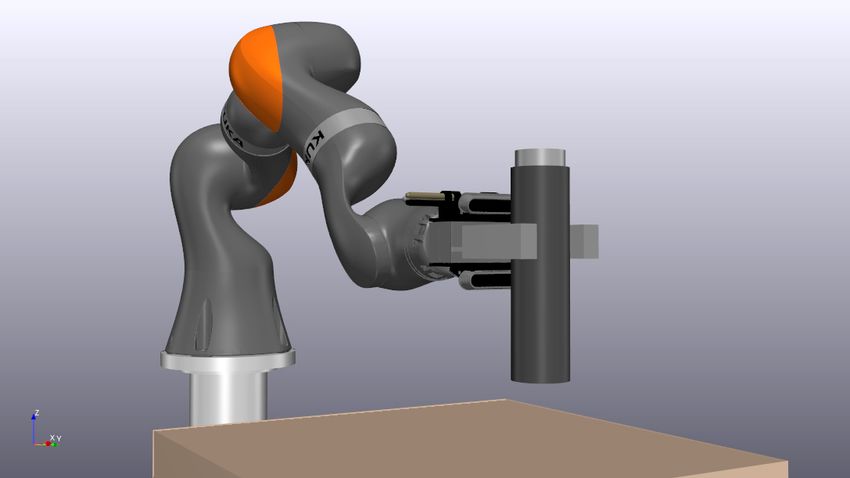
to a linear complementarity problem (LCP) using a polygo-          friction is about τ ≈ vs /g ≈ 10−5 s. We observed in our
nization of the friction cone [7], [8]. LCPs are often solved      simulations that error-controlled integrators must take steps
using direct pivoting methods such as Lemke’s algorithm.           as small as 0.1 µs to resolve these highly stiff dynamics.
Even though there are theoretical results for the solution         As a result, integrators spend most of the computational
of LCPs [9], the class of systems for which they apply are         effort on resolving these unimportant, artificially introduced
seldom found in practice, and robust LCP implementations           dynamics even when common grasping tasks involve much
are either slow or proprietary. The authors of [10] iteratively    larger time scales on the order of tenths of a second. With
solve a quadratic program (QP) for the friction impulses and       implicit integration, stability theory says we should be able
a second QP for the normal impulses. Although the results          to take large time steps once in stiction, even with a very
are promising, the coupled problem is non-convex and the           small vs . That has proven difficult in practice, however. In
solution is not guaranteed to exist.                               this work, we analyze the cause and present methods that
   Another drawback of LCP formulations is that the lin-           enable the realization of this theoretical promise in practice.
earization of the friction cone might lead to preferential            We organize our work as follows. Section II introduces the
directions and cause bias in the solution [11]—an example          mathematical framework and notation. Section III introduces
of a potentially-significant non-physical simulation artifact.     our novel Transition-Aware Line Search (TALS) in the
The computational gain from approximating the friction cone        context of implicit integration. We systematically assess the
is not clear given that the LCP introduces many auxiliary          performance of a variety of integrators using work-precision
variables and constraints, and thus [12] propose to solve the      plots on a series of proposed canonical test problems in
original NCP with a non-smooth Newton method.                      Section IV and measure the improvement in robustness and
   Methods using rigid-body assumptions with Coulomb               performance introduced by TALS. We show TALS performs
friction face the challenging task of solving oftentimes           best when freezing the configuration of the system and
indeterminate, non-convex, and highly nonlinear systems of         propose an original Transition-Aware Modified Semi Implicit
equations. Therefore it is common practice to relax the            (TAMSI) method in Section V. In section VI we show
contact constraints by introducing regularization [13] or          that TAMSI handles transitions robustly and outperforms
softening [14], [15], [16]. This approach allows objects to        our best implicit integrators for the simulation of relevant
interpenetrate by essentially adding numerical compliance.         manipulation tasks. In VI-C we demonstrate our method in
   Given that the true physics of contact involves compliance      a sim-to-real comparison using a Kuka arm manipulation
and many of the approaches using rigid-body assumptions in-        station. Final remarks and possible research directions are
troduce numerical compliance to make the problem tractable,        presented in Section VII.
in this work we instead favor modeling compliant contact
directly. Models in the literature include those for point                II. M ULTIBODY DYNAMICS WITH C ONTACT
contact based on Hertz theory [17], volumetric models [18]           We start by stating the equations of motion and introducing
and more sophisticated approaches modeling the contact             our notation,
patch [19], [20].
                                                                                     q̇ = N(q)v,                               (1)
   By incorporating compliant contact forces with regularized
friction, we can write the system dynamics as a system of                      M(q)v̇ = τ (q, v) +    JTc (q)fc (q, v),        (2)
continuous ordinary differential equations (ODEs). Regular-
                                                                   where q ∈ Rnq and v ∈ Rnv are the vectors of generalized
ization of Coulomb friction replaces the strict friction-cone
                                                                   positions and velocities respectively, M(q) ∈ Rnv ×nv is the
constraint with a smooth function of the slip velocity and
                                                                   system’s mass matrix, τ (q, v) is a vector of generalized
introduces a regularization parameter, or stiction velocity,
                                                                   forces containing Coriolis and gyroscopic terms, gravity,
vs such that true stiction is not possible—objects still slide
                                                                   externally applied forces, and actuation, and Jc and fc are
with a velocity smaller than vs . To simulate manipulation
                                                                   contact Jacobians and forces, defined in Section II-A. We
tasks, this sliding must be made negligible by choosing
                                                                   explicitly emphasize the functional dependence of fc (q, v)
small values of the regularization parameter, typically vs ≤
                                                                   on the state vector x = (q, v) given that we use a compliant
10−4 m/s. The resultant ODE system is stiff and stable
                                                                   contact model with regularized friction. Finally, N(q) ∈
integration requires either very small time steps or implicit
                                                                   Rnq ×nv in Eq. (2) is a block diagonal matrix describing
integration.
                                                                   the kinematic mapping between generalized velocities v and
   Robotic grippers and hands often have soft surfaces to
                                                                   time derivative of generalized positions q̇. Together, Eqs. (1)
increase the efficiency of the grasping system. Therefore the
                                                                   and (2) describe the system’s dynamics as
numerical stiffness of the model is not dominated by elastic
forces but by the regularization of friction. Consider a typical                            ẋ = f (t, x).                     (3)
grasping scenario with a parallel gripper such as the one
shown in Fig. 6 and a model with a regularization parameter        A. Kinematics of Contact
of vs ≈ 10−4 m/s. In static equilibrium, the forces due to           In point contact, contact between sufficiently smooth non-
friction balance the pull of gravity which would otherwise         conforming surfaces can be simply characterized by a pair of
accelerate the object downwards at g ≈ 9.8 m/s2 . There-           witness points Aw and Bw on bodies A and B, respectively
fore the characteristic time scale introduced by regularized       such that Aw is a point on the surface of A that lies the
farthest from the surface of B and vice versa. At the ith As with velocities, we group contact forces fc,i into a
contact we define the contact point Ci to be midway between single vector fc (q, v) ∈ R3nc . We split the contact forces in
the witness points. For a given configuration q of the system their normal and tangential components as fc = fn + ft and
each contact point is characterized by a penetration distance define the generalized forces due to contact as τn (q, v) =
δi (q) and a contact normal n̂i (q) defined to point from JTc (q)fn (q, v) and τt (q, v) = JTc (q)ft (q, v). We note that,
body B into body A. We denote with vc,i the velocity of since ft = P⊥ n ft we can write
witness point Aw relative to Bw , which can be uniquely
split into normal velocity vn,i = Pn,i vc,i and tangential τt (q, v) = JTc (q) ft (q, v),
= JTc (q) P⊥
⊥
velocity vt,i = Pn,i vc,i where Pn,i = n̂i ⊗ n̂i and n (q)ft (q, v) ,
⊥
Pn,i = I −Pn,i are symmetric positive semi-definite (SPSD) = P⊥
T
n (q)Jc (q) ft (q, v),
projection matrices in R3×3 .
For a state with nc contact points we group the velocities = JTt (q)ft (q, v). (8)
vc,i of all contact points in a vector vc ∈ R3nc . In Eq. III. I MPLICIT I NTEGRATION WITH TALS
(2) the contact Jacobian Jc (q) ∈ R3nc ×nv maps generalized
We introduce our Transition-Aware Line Search (TALS)
velocities to contact point velocities as vc = Jc v. We group
method to improve the convergence and robustness of im-
the scalar separation velocities vn,i = n̂i · vc,i into a vector
plicit integration methods when using large time steps in
vn ∈ Rnc so that vn = Jn v, where Jn = N̂T Jc ∈ Rnc ×nv
multibody models with compliant contact and regularized
is the normal velocities Jacobian and N̂ = diag({n̂i })
friction. To describe our method, we make a brief overview
is a block-diagonal matrix in R3nc ×nc . For the tangential
of the implicit Euler method, though TALS can be used
velocities we write
with other implicit integrators. Consider a discrete step of
vt (q, v) = Jt (q)v, (4) size h from time tn−1 to time tn = tn−1 + h. Implicit
Euler approximates the time derivative in Eq. (3) using a
with Jt (q) = P⊥ n (q)Jc (q) ∈ R
3nc ×nv
the Jacobian of first order backward differentiation formula. The resulting
⊥ ⊥
tangential velocities and Pn (q) = diag({Pn,i }) a block system of equations is nonlinear in xn and can be solved
3nc ×3nc
diagonal matrix in R . The reader should notice the using Newton’s method,
difference in sizes for vn ∈ Rnc grouping the scalar sepa- −1
ration velocities, and for vt ∈ R3nc grouping 3D tangential ∆xk = − Ak r(xn,k );
velocities. This choice simplifies the exposition that follows. xn,k+1 = xn,k + ∆xk , (9)
B. Compliant Contact with Regularized Friction where k denotes the iteration number, the residual is defined
The normal component of the contact force is modeled as r(x) = x − xn−1 − h f (x), and Ak = ∇x r(xk ) is the
following the functional form proposed in [21], which is Jacobian of the residual. We use the integrators implemented
continuous in both penetration distance δi and rate δ̇i as in Drake [22] which use the stopping criterion outlined in
[23, §IV.8] to assess convergence of Newton iterations.
πi = ki (1 + di δ̇i )+ δi+ , (5)
A. Transition-Aware Line Search
where (·)+ = max(·, 0) and ki and di are stiffness and
damping parameters. Thus, the normal component of the We observed the Newton iteration in Eq. (9) most often
contact force on body A applied at point Ci is fn,i = πi n̂i . fails during slip-stick transitions when using large time steps
These parameters can be treated as either physical parameters given that Ak in the sliding region, kvt,i k > vs , is not a good
computed for instance according to the theory of Hertz approximation of Ak in the stiction region, kvt,i k < vs . This
contact as in [19] or as numerical penalty parameters as problem is illustrated in Fig. 2 for a 1D system, showing
in [14], [22]. Since the penetration distance δi is defined the Newton residual as a function of sliding velocity. Notice
positive for overlapping geometries, its time derivative relates the sharp gradient in the region kvt,i k < vs due to the
to the separation velocity vn,i by δ̇i = −vn,i . regularization of friction. An iterate with positive velocity
We approximate the Coulomb friction force on body A at v0 will follow the slope to point v1 on the negative side.
Ci with a linear functional form of the tangential velocity Given the transition into the stiction region is missed, next
vt,i , though smoother functions can be used iteration then follows the slope to v2 once again on the
positive side. Subsequent iterations continue to switch back
ft,i = −µ̃i (kvt,i k/vs ) πi v̂t,i , (6) and forth between positive and negative velocities without
(
µi s, 0 ≤ s ≤ 1, achieving convergence. We found this can be remediated by
µ̃i (s) = (7) limiting an iteration crossing the stiction region to fall inside
µi , 1 < s,
of it. As soon as Ak is updated with the more accurate,
where µ̃(s) ≥ 0 is the regularized friction coefficient with and larger, value within the stiction region, Newton iterations
µi the coefficient of friction and vs , with units of velocity, proceed without difficulties.
is the regularization parameter. We show in Section V-A that Similar to other system-specific line search approaches
regularized friction with positive slopes, i.e. µ̃0 (s) ≥ 0 leads [12], [24], for three dimensional problems TALS limits the it-
to considerably more stable integration schemes. eration update in Eq. (9) according to xn,k+1 = xn,k +α∆xkr(v)
vs vs
v1
v0 v2 v
v
*
Fig. 3: TALS limits the update of tangential velocities for
Fig. 2: Divergence of Newton-Raphson near stiction. Itera-
the next Newton iteration when it detects transitions through
tions cycle between v2 and v1 indefinitely.
the stiction region (left). We found that limiting updates to
a maximum angle θMax increases robustness (right).
where α ∈ [0, 1]. If we freeze the configuration q in Eq. (4),
this is equivalent to limiting the tangential velocity of each
n,k+1 n,k k understand if it is worth paying the additional cost of error-
contact point according to vt,i = vt,i + α∆vt,i , with
k controlled integration. We accomplish this by creating so-
∆vt,i the change predicted by Eq. (9), see Fig. 3. We monitor
called work-precision plots that measure cost vs. precision
transition to stiction by detecting the moment at which the
in the solution. We use the number of evaluations of the
line connecting two iterations intersects the stiction region,
system’s dynamics f (t, x) as a metric of work, including
inspired from the idea used in [25] to compute incremental
the evaluations used to approximate the Jacobian of f (t, x)
impulses for impact problems.
through forward differencing. For precision we want a metric
TALS proceeds as follows: given a pair of iterates xn,k
that measures global error while avoiding undesirable drifts
and xn,k+1 from Eq. (9), we update tangential velocities
observed over large periods, especially when using first order
according to Eq. (4). At the ith contact point, if the line
n,k n,k+1 methods. Therefore we localize our global error metric by
connecting vt,i and vt,i crosses the stiction region, we
n,k+1 k
quantifying it within a time window ∆w . To be more precise,
compute αi so that vt,i · ∆vt,i = 0. Even if transition Rτ
we introduce the flow map y = Φτ (x0 ) such that y = 0 f dt
is not detected, we also limit large angular changes between with initial condition y(0) = x0 . We compute a solution
n,k n,k+1
vt,i and vt,i to a maximum value θMax , see Fig. 3. In xm with the method under test at discrete times tm spaced
practice we found the angular limit to increase robustness by intervals of duration ∆w . We then compute a localized
and use θMax = π/3. We finally compute the global TALS reference solution defined by xm m−1
r = Φ∆w (x ), where
limiting parameter as α = min({αi }). notice we use the test solution x m−1
as the initial condition
of the reference solution xmr for the next time window ∆w .
B. Implementation Details
In practice we integrate xmr numerically with a much higher
We incorporate TALS in the implicit integrators imple- precision than the errors in the solution we want to measure.
mented in Drake [22]. Drake offers error-controlled integra- Finally, we make an error estimate by comparing x with the
tion to a user-specified accuracy a, which translates roughly reference xr , see below.
to the desired number of significant digits in the results.
We can also control whether to use a full- or quasi-Newton A. Performance Results with a Small System
method with Jacobian update strategies as outlined in [23, We choose a simple 2D box system that exhibits periodic
§IV.8]. stick-slip transitions. The box of mass m = 0.33 kg lies
We make the distinction between error-controlled and on top of a horizontal surface with friction µ = 1.0 and
convergence-controlled integration, which retries smaller is forced to move sideways by an external harmonic force
time steps when Newton iterations fail to converge, as f (t) of amplitude 4 N and a frequency of 1 Hz. The system’s
described in [23, §IV.8]. All of our fixed-step integrators dynamics for this case reduces to mv̇ = f (t)−µ̃(v)W sgn(v),
use convergence control. We refer interested readers to the with W the weight of the box in Earth’s gravity of g =
accompanying documentation in Drake [22] for details. 9.8 m/s2 and µ̃(v) as defined in Eq. (7) with vs = 10−4 m/s.
Using a fixed time step h = 10 ms, much larger than
IV. I NTEGRATION P ERFORMANCE
the time scale introduced by regularized friction, we observe
In this section, we evaluate TALS with fixed-step and Newton iterations not to converge as described in Section III-
error-controlled implicit Euler (IE) integrators. The precision A. Figure 4 shows the Newton residual history the first time,
obtained with fixed-step integrators is controlled via the time at t = 0.160 s, the box transitions from sliding into stiction.
step size h. In contrast, error-controlled integrators adjust TALS is able to detect transition, properly limit the iteration
the time step size to meet a user-specified accuracy a, with update and even recover the second order convergence rate
additional overhead for local error estimation. of Newton’s method.
Our objective is to evaluate the trade-off between perfor- Figure 5 shows a work-precision plot with an error
mance and precision for a variety of integration methods and estimate ev in the horizontal velocity v defined as theB. Performance with Larger Systems
0.2
0.1
When we applied TALS with implicit Euler to systems
v t [m/s]
with more degrees of freedom, we found TALS to be highly
0
sensitive to changes in the configuration q of the system.
-0.1
Specifically, we observed iterations during which tangential
-0.2
velocities fall outside the region kvt k < vs even after TALS
0 5 10 15 20
10 0 Newton-Raphson Iteration Count
detects a transition and limits the Newton update. We traced
this problem to changes in the tangential velocities Jacobian
Jt (q) in Eq. (4) caused by small changes to the configuration
| v t | [m/s]
10 -10 q. These iterations during transition steps often result in the
same convergence failure as experienced by integrators with-
out TALS (Figure 4), leading to a performance deterioration.
10 -20
0 5 10 15 20
Newton-Raphson Iteration Count V. T RANSITION -AWARE S EMI -I MPLICIT M ETHOD
Fig. 4: Newton’s method misses stiction, oscillates, and does We draw from the lessons learned in the previous section
not converge (top). TALS detects the transition to stiction, to design a scheme customized for the solution of multibody
limits the iteration update, and guides Newton’s method to dynamics with compliant contact and regularized Coulomb
convergence (bottom). friction. Based on the observation that TALS is sensitive to
changes in the system configuration q, we decided to freeze
the configurations in Eq. 2 so that we could iterate on the
generalized velocities without changes in the configuration
10 7
affecting the stability of TALS. An important computational
FN
advantage of this approach is that the typically demanding
Number of Function Evaluations [-]
FN+TALS
EC+FN geometric queries only need to be performed once at the
10 6 EC+FN+TALS
QN beginning of the time step.
QN+TALS
EC+QN
This is the same idea behind the semi-implicit Euler
EC+QN+TALS scheme. This scheme however becomes unstable for stiff
10 5
contact forces in the normal direction since the position
dependent terms are treated explicitly as in the conditionally
stable explicit Euler scheme. Our TAMSI scheme deals
10 4 with this problem by introducing an implicit first order
approximation of the penetration distances with generalized
velocities.
10 3 We will introduce TAMSI in stages so that we can analyze
10 -1 10 0 10 1 10 2
Slip Velocity Error (e v / v s) [-] the properties of different contributions separately. We start
with the traditional semi-implicit Euler and highlight the
Fig. 5: We evaluate implicit Euler integration performance differences as we progressively introduce TAMSI.
with full- (FN) and quasi- (QN) Newton updates, each with
A. Semi-Implicit Euler: One-Way Coupled TAMSI Scheme
and without error control (EC), and with and without TALS.
The semi-implicit Euler scheme applied to Eqs. (1)-(2)
effectively freezes the normal contact forces to fn,0 . In this
L2 -norm of the difference between the solution {v m } and regard the scheme is one-way coupled, meaning that normal
the reference solution {vrm }. We use a localized global error forces couple in the computation of friction forces but not
estimate computed with ∆w = 25 ms and a reference the other way around.
solution computed by a 3rd order Runge-Kutta with fixed Using a time step of length h, the semi-implicit Euler
step of h = 10−7 s. Each point in this figure corresponds to scheme applied to Eqs. (1)-(2) reads,
a different accuracy a when using error control, or a different q = q0 + N0 v, (10)
time step h when using fixed steps. The same error metric ∗
in the horizontal axis allows for a fair comparison. M0 v = p + hJTc,0 fc (q0 , v), (11)
We observe the expected theoretical first order slope for where the naught subscript in q0 , v0 , M0 = M(q0 ), JTc,0 =
errors near vs or smaller. However, for errors larger than vs , JTc (q0 ), and N0 = N(q0 ) denotes quantities evaluated at the
integrators without TALS depart from the theoretical result previous time step. To simplify notation we use bare q and
as their performance degrades. Figure 5 shows that TALS v to denote the state at the next time step. We defined p∗ =
improves performance by extending the range in which the M0 v0 +hτ (q0 , v0 ) as the momentum the system would have
first order behavior is valid, up to a factor of 10 (FN) or 3 on the next time step if contact forces were zero. Since we are
(QN). interested in low-speed applications to robotic manipulation,the gyroscopic terms in p∗ are treated explicitly. It is known the normal forces as fn (vn ) = N̂0 π(vn ). This can then be
however that for highly dynamics simulations, more robust used in Eq. (18) to compute the Jacobian of the residual,
approaches should treat these terms implicitly [26].
∇v r(v) = M0 − h JTc,0 ∇v fn (vn ),
A semi-implicit Euler scheme solves Eq. (11) for v at the
next time step and uses it to advance the configuration vector = M0 − h JTc,0 ∇vn fn (vn ) Jn,0 ,
q to the next time step with Eq. (10). One disadvantage is = M0 − h JTc,0 N̂0 ∇vn π(vn ) Jn,0 ,
that this approach often becomes unstable because the stiff = M0 + h Wnn,0 , (20)
compliant normal forces are explicit in the configuration q.
To solve Eq. (11) we define the residual where we introduced the normal direction Delassus oper-
ator Wnn,0 = −JTn,0 ∇vn π(vn ) Jn,0 and ∇vn π(vn ) =
r(v) = M0 v − p∗ − hτn,0 − hτt (q0 , v), (12) diag({dπi /dvn,i }). With the compliant contact model in Eq.
(5) we have dπi /dvn,i ≤ 0 and therefore the Delassus
and use its Jacobian in Newton iterations. The Jacobian is operator Wnn,0 is SPSD. This implies that the Jacobian in
Eq. (20) is SPD and its inverse always exists, explaining the
∇v r(v) = M0 − h∇v τt (q0 , v). (13) high stability of this scheme for contact problems without
Substituting in Eq. (8), friction.
C. TAMSI: Two-Way Coupled Scheme
∇v τt (q0 , v) = JTt,0 ∇v ft (q0 , v), (14)
Using the results from previous sections we are now ready
= JTt,0 ∇vt ft (q0 , v)Jt,0 , (15) to derive our TAMSI scheme. TAMSI is a semi-implicit Euler
scheme in the friction forces as introduced in Section V-A
where we used Eq. (4) and ∇vt ft = diag({∇vt,i ft,i }) ∈ modified to implicitly couple the compliant contact forces
R3nc ×3nc , with each block computed as the gradient with using the approximation in Eq. (19). It is a two-way coupled
respect to vt,i in Eq. (6): scheme in that, in addition to normal forces feeding into the
µ̃(si ) ⊥ µ̃0 (si )
computation of the friction forces through Eq. (6), friction
∇vt,i ft,i = −πi,0 Pn (q) + Pn (q) , (16) forces feedback implicitly into the normal forces.
kvt,i k vs
Freezing the position kinematics to q0 and using the
where µ̃0 (s) = dµ̃/ds. We introduce the tangential direction approximation in Eq. (19), the full TAMSI residual becomes
Delassus operator as Wtt,0 = −JTt,0 ∇vt ft (q0 , v)Jt,0 and r(v) = M0 v − p∗ − h JTn,0 π(vn ) − h JTt,0 ft (vt ). (21)
write the Jacobian of the residual as
We can then use the results from the previous sections,
∇v r(v) = M0 + h Wtt,0 . (17) except we also need to take into account how the friction
forces in Eq. (6) change due to changes in the normal forces.
We note that with the choice of regularization function such Instead of the result in Eq. (15), we now have
that µ̃0 (s) ≥ 0, −∇vt,i ft,i is a linear combination of SPSD
matrices and therefore the Delassus operator Wtt,0 is SPSD. ∇v τt = JTt,0 ∇v ft ,
Thus ∇v r(v) in Eq. (17) is symmetric positive definite = JTt,0 ∇vt ft Jt,0 + JTt,0 ∇vn ft Jn,0 ,
(SPD) and thus its inverse always exists. = −Wtt − Wtn , (22)
3nc ×nc
B. Implicit Approximation to Normal Forces where ∇vn ft = −diag({µ̃i v̂t,i dπi /dvn,i }) ∈ R .
We define the generally non-symmetric operator Wtn =
We present an approximation to treat normal forces im- −JTt,0 ∇vn ft Jn,0 ∈ Rnv ×nv which introduces the additional
plicitly while still keeping the configurations frozen. For two-way coupling between compliance in the normal direc-
simplicity, we consider frictionless contact first tion and friction in the tangential direction.
Using these results we can write the Jacobian of the
r(v) = M0 v − p∗ − h JTc,0 fn (q, v), (18)
TAMSI scheme as
where notice we decided to freeze the contact Jacobian but ∇v r(v) = M0 + h (Wnn,0 + Wtt,0 + Wtn,0 ) . (23)
not the compliant contact forces.
Notice that, due to Wtn,0 , the Jacobian is not symmetric
To treat the normal contact forces implicitly while still
and in general not invertible. However, since M0 is SPD,
freezing the configuration at q0 , we propose the following
the Jacobian is invertible for sufficiently small h.
first-order estimation of the penetration distance δi at the ith After computing the next Newton iteration using this
contact point, Jacobian, we use TALS to selectively backtrack the iteration.
δi ≈ δi,0 − h vn,i , (19)
VI. R ESULTS AND D ISCUSSION
where we used the fact that δ̇i = −vn,i . We can then We present a series of simulation test cases to assess
substitute Eq. (19) into Eq. (5) to express the compliant robustness, accuracy and performance. For all cases we use
forces, πi (vn,i ), as function of the normal velocities and a regularized friction parameter of vs = 10−4 m/s, which
group them into a vector, π(vn ) ∈ Rnc . We then express results in negligible sliding during stiction.100
Rotational Velocity Error
Translational Velocity Error
-1
Normalized Error ( e T, ev T/A) [-]
10 Reference First-Order Line
10-2
10-3
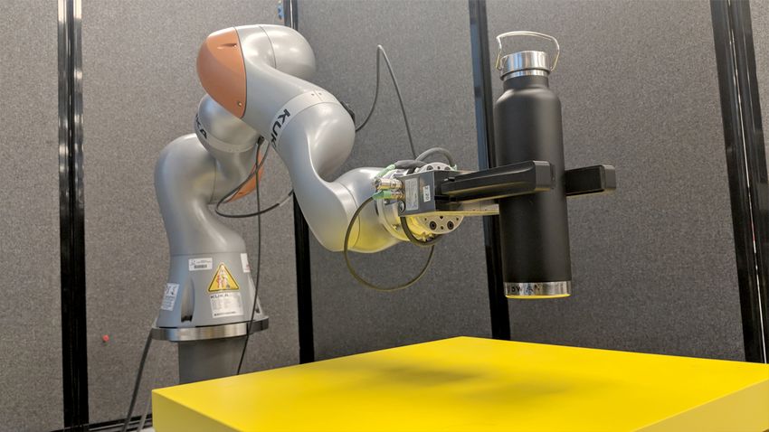
Fig. 6: Parallel jaw gripper model. We shake the mug 10-4
vertically to assess robustness.
10-5
5
10-6 10-4 10-2
Simulation Time [s]
Normalized Step Size (h/T) [-]
4
3 Fig. 8: L2 -norm of the generalized velocity errors against
time step, nondimensionalized with the problem’s period T
2 and amplitude A. Both translational and rotational DOFs
TAMSI
1 IE+FN+TALS exhibit first order convergence as expected.
IE+FN
0
0 1 2 3 4 5 6
CPU Wall Clock Time [s]
Fig. 7: Simulated time vs. wall-clock time for the parallel
jaw gripper case. All three runs use h = 3 ms. TAMSI is the
fastest, on the far left. The horizontal plateaus in the IE+FN
run indicate that without TALS, the integrator slows down
since it takes smaller step sizes for convergence control. Fig. 9: Model of a 16 DOF Allegro hand holding a mug. As
the hand reorients the mug, multiple simultaneous points of
A. Parallel Jaw Gripper contact securing the grasp are made.
To assess the robustness of our method in a relevant ma-
nipulation task with large external disturbances, we simulate We observe that TALS does not improve the performance
a parallel jaw gripper holding a mug and forced to oscillate of implicit Euler — as the system configuration q changes,
vertically with a period of T = 0.5 s and an amplitude of the tangent space reorients, and TALS is unable to properly
A = 15 cm, see Fig. 6. To stress the solver in a situation with control iterations with transitions into stiction. TAMSI how-
slip-stick transitions, we chose a low coefficient of friction ever, with a time step h = 0.7 ms, runs 7.8× faster than our
of µ = 0.1 and a grip force of 10 N. The mug is 10 cm fastest integrator setup, the error-controlled implicit Euler
tall with a radius of 4 cm and a mass of 100 g. There is no using quasi-Newton when solving to a (loose) accuracy of
gravity. a = 0.01 m/s. Our single-threaded TAMSI completes 15
With a step h = 3 ms TAMSI completes 5 seconds seconds simulated time on an Intel i7-6900K 3.2 GHz CPU
of simulation time with a single thread on an Intel i7- in 7.0 s of wall-clock time, or 2.14× real-time rate.
6900K 3.2 GHz CPU in 123 ms of wall-clock time, or
40× real-time rate. In contrast, IE+FN with TALS is 25× C. Sim-to-Real Experiments
slower than TAMSI and IE+FN without TALS is 55× slower We demonstrate our simulation capability with TAMSI in
than TAMSI. Simulated time vs wall-clock time for each is a manipulation task with closed-loop control involving force-
shown in Fig. 7. Next, we perform a convergence study for feedback and manipuland-world contact. We use a Kuka
TAMSI running with different time steps and estimate an IIWA arm (7 DOF) outfitted with a Schunk WSG 50 gripper.
error against a reference TAMSI solution using h = 10−7 s, The robot was commanded to move towards a cylindrical
Fig. 8. As expected, TAMSI exhibits first order convergence manipuland (water bottle), execute a grasp and then perform
with step size. a vigorous shake motion before placing the manipuland
down at a new location, see Fig. 1 and the accompanying
B. Allegro Hand supplemental video.
We simulate a 16 DOF allegro hand controlled in open- We use an inverse dynamics controller with gains in the
loop to perform a periodic reorientation of a mug, see Fig. 9 simulation set to best match reality, even though the specifics
and the supplemental video accompanying this manuscript. of Kuka’s proprietary joint-level controller are unavailable.
This interesting system includes multiple points of contact, The controller process tracks a prescribed sequence of Carte-
complex geometry and a large number of DOFs. sian end-effector keyframe poses and computes desired joint-space trajectories using Jacobian IK. We use force feedback [5] S. Li, S. Lyu, J. Trinkle, and W. Burgard, “A comparative study of
to regulate the grasp force and judge for placement success. contact models for contact-aware state estimation,” in 2015 IEEE/RSJ
International Conference on Intelligent Robots and Systems (IROS).
TAMSI proves to be a robust scheme for this case and IEEE, 2015, pp. 5059–5064.
performs well even during the vigorous shaking motions [6] S. Hogan and K. U. Kristiansen, “On the regularization of impact
performed by the robot while grasping the bottle. Contact without collision: the painlevé paradox and compliance,” Proceedings
of the Royal Society A: Mathematical, Physical and Engineering
results and forces used to emulate force feedback in the Sciences, vol. 473, no. 2202, p. 20160773, 2017.
real robot prove to be of sufficient accuracy to calibrate the [7] D. E. Stewart and J. C. Trinkle, “An implicit time-stepping scheme for
controller in simulation and transfer to reality without any rigid body dynamics with inelastic collisions and coulomb friction,”
International Journal for Numerical Methods in Engineering, vol. 39,
additional parameter tuning. no. 15, pp. 2673–2691, 1996.
[8] M. Anitescu and F. A. Potra, “Formulating dynamic multi-rigid-body
VII. CONCLUSIONS contact problems with friction as solvable linear complementarity
problems,” Nonlinear Dynamics, vol. 14, no. 3, pp. 231–247, 1997.
In this work we systematically analyzed implicit integra- [9] R. Cottle, J. Pang, and R. Stone, The Linear Complementarity Prob-
lem, ser. Computer science and scientific computing. Academic Press,
tion for multibody problems with compliant contact and reg- 1992.
ularized friction. Error-controlled implicit Euler with quasi- [10] D. M. Kaufman, S. Sueda, D. L. James, and D. K. Pai, “Staggered
Newton iterations performs best, though it spends a signifi- projections for frictional contact in multibody systems,” ACM Trans-
actions on Graphics (TOG), vol. 27, no. 5, p. 164, 2008.
cant amount of time resolving the high-frequency transition [11] J. Li, G. Daviet, R. Narain, F. Bertails-Descoubes, M. Overby, G. E.
dynamics introduced by regularized friction. Our new TALS Brown, and L. Boissieux, “An implicit frictional contact solver for
method helps to address this problem, though its performance adaptive cloth simulation,” ACM Transactions on Graphics (TOG),
vol. 37, no. 4, p. 52, 2018.
degrades as the configuration of the system changes and [12] E. Todorov, “Implicit nonlinear complementarity: A new approach
contact surfaces reorient. This observation led us to develop to contact dynamics,” in 2010 IEEE International Conference on
our novel TAMSI method. TAMSI approximates penetration Robotics and Automation (ICRA). IEEE, 2010, pp. 2322–2329.
[13] C. Lacoursiere and M. Linde, “Spook: a variational time-stepping
distances to first-order to couple contact forces implicitly scheme for rigid multibody systems subject to dry frictional contacts,”
while performing only a single geometric query at the Umeå University, UMINF report 11.09, 2011.
beginning of a time step, resulting in improved performance. [14] E. Catto, “Soft constraints: Reinventing the spring,” in Game Devel-
oper Conference, 2011.
We demonstrate the added robustness and performance of [15] E. Coumans, “Bullet physics library,” 2015. [Online]. Available:
TAMSI with simulations of relevant manipulation tasks. A http://bulletphysics.org
sim-to-real comparison shows a usage of TAMSI to prototype [16] R. Smith, “Open dynamics engine.” [Online]. Available: http:
//www.ode.org
a controller in simulation that transfers effectively to reality. [17] L. Luo and M. Nahon, “A compliant contact model including interfer-
Additional examples are available in the open-source ence geometry for polyhedral objects,” Journal of Computational and
robotics toolbox Drake [22]. Ongoing work conducted at the Nonlinear Dynamics, vol. 1, no. 2, pp. 150–159, 2006.
[18] Y. Gonthier, “Contact dynamics modelling for robotic task simulation,”
Toyota Research Institute is leveraging the proposed method Ph.D. dissertation, University of Waterloo, 2007.
for prototyping and validating controllers for robot manip- [19] M. A. Sherman, A. Seth, and S. L. Delp, “Simbody: multibody
ulation in dense cluttered environments [27] and extending dynamics for biomedical research,” Procedia Iutam, vol. 2, pp. 241–
261, 2011.
TAMSI to work with more sophisticated contact models [20]. [20] R. Elandt, E. Drumwright, M. Sherman, and A. Ruina, “A pressure
field model for fast, robust approximation of net contact force and
ACKNOWLEDGMENTS moment between nominally rigid objects,” in 2019 IEEE/RSJ Interna-
tional Conference on Intelligent Robots and Systems (IROS). IEEE,
Ante Qu contributed to this project as an intern at Toyota 2019.
Research Institute. We thank Allison Henry and Siyuan [21] K. H. Hunt and F. R. E. Crossley, “Coefficient of restitution interpreted
as damping in vibroimpact,” Journal of Applied Mechanics, vol. 42,
Feng for technical support, and Evan Drumwright and Russ no. 2, pp. 440–445, 1975.
Tedrake for helpful discussions. [22] R. Tedrake and the Drake Development Team, “Drake: Model-based
design and verification for robotics,” 2019. [Online]. Available:
https://drake.mit.edu
R EFERENCES [23] E. Hairer, S. Nørsett, and G. Wanner, Solving Ordinary Differen-
tial Equations II. Stiff and Differential-Algebraic Problems, 2nd ed.
[1] K. Bousmalis, A. Irpan, P. Wohlhart, Y. Bai, M. Kelcey, M. Kalakr- Springer, 01 1996, vol. 14.
ishnan, L. Downs, J. Ibarz, P. Pastor, K. Konolige, et al., “Using [24] Y. Zhu, R. Bridson, and D. M. Kaufman, “Blended cured quasi-newton
simulation and domain adaptation to improve efficiency of deep for distortion optimization,” ACM Transactions on Graphics (TOG),
robotic grasping,” in 2018 IEEE International Conference on Robotics vol. 37, no. 4, p. 40, 2018.
and Automation (ICRA). IEEE, 2018, pp. 4243–4250. [25] T. K. Uchida, M. A. Sherman, and S. L. Delp, “Making a meaningful
[2] Y. Chebotar, A. Handa, V. Makoviychuk, M. Macklin, J. Issac, impact: modelling simultaneous frictional collisions in spatial multi-
N. Ratliff, and D. Fox, “Closing the sim-to-real loop: Adapting body systems,” Proceedings of the Royal Society A: Mathematical,
simulation randomization with real world experience,” in 2019 IEEE Physical and Engineering Sciences, vol. 471, no. 2177, p. 20140859,
International Conference on Robotics and Automation (ICRA). IEEE, 2015.
2019, pp. 8973–8979. [26] C. Lacoursière, “Stabilizing gyroscopic forces in rigid multibody
[3] S. Kolev and E. Todorov, “Physically consistent state estimation and simulations,” Umeå University, UMINF report 06.05, 2006.
system identification for contacts,” in 2015 IEEE-RAS 15th Interna- [27] R. Tedrake, “TRI taking on the hard problems in manipulation
tional Conference on Humanoid Robots (Humanoids). IEEE, 2015, research toward making human-assist robots reliable and
pp. 1036–1043. robust,” June 2019. [Online]. Available: https://www.tri.global/
[4] D. J. Duff, T. Mörwald, R. Stolkin, and J. Wyatt, “Physical simulation news/tri-taking-on-the-hard-problems-in-manipulation-re-2019-6-27
for monocular 3d model based tracking,” in 2011 IEEE International
Conference on Robotics and Automation (ICRA). IEEE, 2011, pp.
5218–5225.You can also read