Acoustic Based Position Estimation of an Object and a Person Using Active Localization and Sound Field Analysis - MDPI
←
→
Page content transcription
If your browser does not render page correctly, please read the page content below
Article

Acoustic‐Based Position Estimation of an Object
and a Person Using Active Localization and Sound
Field Analysis
Kihyun Kim 1,2, Semyung Wang 1,*, Homin Ryu 2 and Sung Q. Lee 3
 1 School of Mechanical Engineering, Gwangju Institute of Science and Technology (GIST),
   Gwangju 61005, Korea; kihyunkim@gist.ac.kr or khyun.kim@lge.com
 2 Chief Technology Officer, LG Electronics, Seoul 06763, Korea; homin.ryu2@gmail.com

 3 Intelligent Sensors Research Section, Electronics Telecommunication Research Institute (ETRI),

   Daejeon 34129, Korea; hermann@etri.re.kr
 * Correspondence: smwang@gist.ac.kr; Tel.: +82‐62‐715‐2390

 Received: 31 October 2020; Accepted: 16 December 2020; Published: 18 December 2020

 Abstract: This paper proposes a new method to estimate the position of an object and a silent person
 with a home security system using a loudspeaker and an array of microphones. The conventional
 acoustic‐based security systems have been developed to detect intruders and estimate the direction
 of intruders who generate noise. However, there is a need for a method to estimate the distance and
 angular position of a silent intruder for interoperation with the conventional security sensors, thus
 overcoming the disadvantage of acoustic‐based home security systems, which operate only when
 sound is generated. Therefore, an active localization method is proposed to estimate the direction
 and distance of a silent person by actively detecting the sound field variation measured by the
 microphone array after playing the sound source in the control zone. To implement the idea of the
 proposed method, two main aspects were studied. Firstly, a signal processing method that estimates
 the position of a person by the reflected sound, and secondly, the environment in which the
 proposed method can be operated through a finite‐difference time‐domain (FDTD) simulation and
 the acoustic parameters of early decay time (EDT) and reverberation time (RT20). Consequently, we
 verified that with the proposed method it is possible to estimate the position of a polyvinyl chloride
 (PVC) pipe and a person by using their reflection in a classroom.

 Keywords: active localization; acoustic‐based security system; steered response power; sound field
 analysis; finite‐difference time‐domain

1. Introduction
     With the rapid development of smart homes and voice‐assistant technologies, home
environments have been established in which loudspeakers and microphones are deployed as
sensors or are built‐in and distributed through home appliances. The aim of this research was to
develop an acoustic‐based home security system in the aforementioned environment. An example is
shown in Figure 1.
     Smart home technology has been evolving to provide proactive services through the monitoring
of residents. Therefore, accurately recognizing the scenario in a home environment through a
combination of various sensors is important. In [1], studies on context awareness for indoor activity
recognition using binary sensors, cameras, radio‐frequency identification, and air pressure sensors
were reviewed.

Appl. Sci. 2020, 10, 9090; doi:10.3390/app10249090                               www.mdpi.com/journal/applsci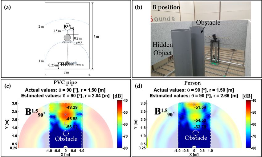
Appl. Sci. 2020, 10, 9090                                                                               2 of 25

      Figure 1. Conceptual illustration of an active localization system based on acoustic sensors in home
      appliances.

     A study proposed to recognize each living activity of a user by combining the power meters of
appliances with an ultrasonic sensor [2]. In [3], a study was conducted to recognize the complex
activities of a kitchen using one module with various sensors.
     In such a smart home environment, microphones are used for context awareness and health
monitoring owing to their advantage of operating with low power [4]. Dahmen et al. explained that
a microphone can be used to identify the scenario of a home environment based on unusual loud
noise and the sound of a human falling [5]. In addition, a study explored the possibility of personal
identification through footsteps [6].
     Automated home security systems have been developed using smart home technologies. Recent
home security systems protect residents and their properties, making them safe from intruders as
conventional security systems, and they enable the detection of risks to the residents in advance
through context awareness of the home environment [5,7].
     Microphones in a home security system are primarily used for two purposes: event detection
and the classification of unusual sounds, and intrusion detection.
     In [8], related studies were reviewed through a comprehensive survey of background
surveillance, event classification, object tracking, and situation analysis, and the detection of events
in a highly noisy environment was proposed [9]. In [10–12], a microphone array and security camera
were combined to detect the sound from an intruder and tilt the security camera in the direction of
the sound. Research has been conducted to predict the state of a control space by recognizing the type
of sound, analyzing and classifying the sound, and estimating the angular position of the unusual
sound using a microphone array [13,14]. A method to identify human behavior in a control space by
applying a microphone array to a sound‐steered camera was proposed [15].
     Intrusion detection using microphones is as effective as the use of security cameras in terms of
detecting moving objects [4], and the related studies are summarized below. Studies on intrusion
detection have been conducted to determine an intrusion in a security zone based on the change in the
room transfer function [16], the sound field variation according to the acoustical transmission path of
distributed microphones [17], and the coherence responses in low‐frequency environments [18].
     However, the conventional methods for event detection have the disadvantage of operating only
when a loud noise is generated because the position is determined in the direction of the generated
sound, and current techniques for intrusion detection have the disadvantage of only detecting
intrusion but not providing the location.
     To overcome these disadvantages, we propose an acoustic‐based active localization and analysis
method to estimate a silent intruder. This study provides a link between localization and intrusion
detection techniques using an acoustic‐based security system. The reason is that if a person’s position
can be estimated and tracked using microphones and loudspeakers, the entry of an unauthorized
Appl. Sci. 2020, 10, 9090                                                                             3 of 25

person into the security space can be known. However, this study primarily addressed the estimation
of the position of a silent intruder.
      The process of a home security system can be divided into sensing, assessing, and responding.
Sensing is very important because it functions as a trigger to operate the security system. Thus, the sensors
must be interoperable with each other [5], with a combination of various individual sensors [5,7], or with
the information measured by one sensor module [19].
      Therefore, through this study, we expected to increase the utilization of microphones used in
home security systems. This is because the data measured by a conventional linear microphone array
provide only angular information. However, the proposed method also provides the distance, which
increases the number of scenarios that can be combined with the information of other sensors.
      We present two examples of complementary sensing. In the first one, passive infrared (PIR)
sensors function as triggers to awake the security system and record the intrusion using a camera [20].
However, PIR sensors have the disadvantage of being unable to detect an intruder who does not move,
moves slowly, or uses heat‐insulating clothes. IR sensors have limitations that often cause errors
because of their nonlinear sensitivity and the effects of nearby objects [21]. Therefore, if the acoustic‐
based intrusion detection in [16–18] is applied to the security system to compensate for the weakness in
IR sensors, the two sensing systems can complement each other to increase the robustness of the
intrusion detection. In the second example, when a microphone array detects the direction of an event,
a pan‐tilt‐zoom (PTZ) camera is rotated and focused on the region of interest [8]. However, because the
camera has misrecognitions owing to poor resolutions, distant targets, changes in illuminations, or
occlusions [22], the PTZ camera can be operated robustly by providing a distance and an angle of the
intruder based on the proposed method.
      Therefore, to overcome the shortcomings of conventional acoustic‐based intrusion detection
systems and achieve the complementary intrusion detection system proposed in [5], this paper
describes our proposed active localization method that estimates the position (distance and angle) of
a silent intruder using a generated reflection. The main concept is that a loudspeaker generates a
signal in the security space. The microphone array extracts the changed signals owing to the intruder,
and then the distance and direction are estimated using the changed signals (sound field variation).
      Echolocation is a technology that detects a location through an echo which is emitted from a
sound source and then returns, and it has been primarily implemented using an ultrasonic sensor. In
[23], a biomimetic sonar system was mounted on a robot arm to recognize an object through the
vector of the echo envelope. A biomimetic study was conducted to estimate the distance and angle
[24]. The distance was estimated using the time delay between the maximum activity owing to the
call and the activity owing to the echo, and the angle was predicted by comparing the directivity
pattern of the sensor using the notch pattern in the frequency range. Ultrasonic sensors are acoustic
sensors used in conventional home security systems. Ultrasonic sensors are active sensors that send
signals in a straight line; therefore, the source and receiver can be placed face‐to‐face [21] or in the
same direction to physically detect the intruder [25]. However, owing to the straightness of the signal,
they have the disadvantages of utilizing several sensors to increase the detection rate [26] and being
unable to detect a person that passes behind an obstacle.
      The proposed active localization in the audible frequency utilizes the phenomenon of scattering
rather than straightness. Through fundamental research, we verified that the scattering phenomenon
in the audible frequency can be used to detect an object [27] or a person hiding behind an obstacle
(the related results are described in Appendix B).
      We expect that the combination of ultrasound with its straightness and audible sound with
strong scattering can detect a person better. Thus, to create a function as a sensor using a loudspeaker
and a microphone array, we studied which room conditions result in the reflection generated by an
intruder being considered as a new sound source.
      We introduce two main topics to implement the proposed idea. The first aspect is signal
processing to estimate the position using reflection, and the second involves the simulation and
analysis method of the sound field to estimate the position through the reflected sound in the
reverberation space. Thus, analysis equations using acoustic parameters are proposed.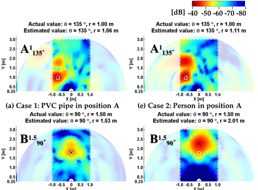
Appl. Sci. 2020, 10, 9090 4 of 25
When estimating the position of a person using an active acoustic‐based method, the analysis of
the sound field to determine the position of the intruder has the following implications. In a
reverberant environment, the proposed method is not aimed at estimating the position by increasing
the number of microphones. In other words, this does not mean that many microphones are
distributed in the control space or that the microphone arrays are arranged at each corner of the
control space. By using limited hardware, one loudspeaker and one microphone array, the method
of estimating a person’s position using the reflected sound is possible through sound field analysis.
Therefore, the active localization method proposed in this paper was verified by estimating the
position of a polyvinyl chloride (PVC) pipe and a person in a classroom using signal processing and
sound field analysis.
The remainder of this paper is organized as follows. In Section 2, the signal model for position
estimation using the reflection sound is presented; subsequently, the algorithm is proposed. The
feasibility results of the proposed method are presented through the testing of an anechoic chamber.
In Section 3, the simulation results for a reverberant environment are described, and the operating
conditions in the reverberant space are proposed based on acoustic parameters. In Section 4, the
examination of the proposed method using a PVC pipe and a person in a classroom is described.
Finally, the conclusions are presented in Section 5.
2. Implementation of Active Localization: Signal Model, Processing, and Feasibility Test
2.1. Signal Model and Definition of Sound Field Variation
The implementation of active localization to estimate the position of a silent intruder requires a
reflected sound generated by a silent intruder. We define the sound field variation as the difference
between the sound field before intrusion and the sound field after intrusion.
Therefore, the proposed active localization based on the sound field variation can be tested using
two steps. The first step is to measure the sound field in a targeted security space using an active
approach with a loudspeaker and a microphone array. The second step is to obtain the position of
the silent intruder by acquiring the signals of the sound field variation based on a comparison
between the signal of the sound field before intrusion (the reference sound field) and after intrusion
(the event sound field).
Figure 2 shows the scheme of sound field variation and, as an example, shows some of the
reflections. Because the proposed active localization method uses the time signals from a direct sound
to the early reflections and we assume that the silent intruder affects the specific reflection locally,
we define the decomposition of room impulse responses as in Equations (1) and (2).
Figure 2. Scheme of sound field variation between (a) a reference scenario and (b) an event scenario:
(a) Early reflection of room impulse response in a reference scenario without an intruder; (b) early
reflection of room impulse response in an event scenario with an intruder.
Equations (1) and (2) represent the decomposition of the room impulse response (RIR) of the
reference and intruder scenarios in the time domain, respectively.
h ref = h s + h r1 + + h r n + h reverberation (1)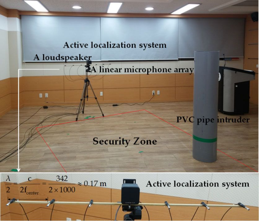
Appl. Sci. 2020, 10, 9090 5 of 25
h event = h s + α 1 h r1 + + α n h r n + h person + h reverberation (2)
where h re f is the RIR of a reference scenario, hevent is the RIR of an event scenario, h r n represents
the early reflections of each scenario, h person is the new response generated by a person, h reverberation is
the late reverberation of the room impulse response, and α n represents the attenuation coefficients.
Methods to estimate the room shape or locate a sound source by analyzing the echo components
of the RIR have been proposed [28–30]. However, because these methods are performed assuming
that the RIR is known, the problem of measuring RIR every time an intruder moves in a scenario
exists, and they have the disadvantage of being slow systems.
Therefore, in this study, the signal modeling was represented by the viewpoint of the echo
decomposition of the RIR, but the signal generated by the loudspeaker was determined using the
Gaussian‐modulated sinusoidal pulse in Equation (10) to analyze the changed sound field before and after
the intrusion, and the extraction of the changed echo component was performed using Equation (3).
If the silent intruder affects the reflection h r n of the RIR locally, the sum of early reflections in
an event scenario is approximate to the sum of early reflections in a reference scenario, i.e.,
α1 α 2 α n 1 . Therefore, Equation (2) can be rewritten as Equation (3).
h event = h ref + h person + error (3)
The sound field variation can be calculated using Equation (4).
Gm Ym Gm ‐ Ym R effect
ΔHm = Hevent
m ‐ Href
m = ‐ = = m (4)
X X X X
where Href
m
is the transfer function of the control area under the reference scenario shown in Figure
2a, H event
m is the transfer function under the event scenario shown in Figure 2b, X is the input signal,
Gm represents the signals measured by the microphone array after an intrusion, Ym represents the
reference signals before an intrusion, R effect
m
represents the changed spatial effects, and m is a
microphone index.
The spatial effects R effect
m
are assumed to include the sound signals emitted as reflections by the
silent intruder. In other words, R effect
m
can be assumed to also consider the new sound source. This is
because the intruder changes the sound field formed from the sound source of a loudspeaker, and
then the intruder’s position is estimated using the measured R effect
m
at a microphone array. This is the
same concept in which the incident, reflected, and transmitted phenomena of pressure distribution
on the flat surface of a discontinuity are considered to be the sum of the blocked pressure and the
radiation pressure in [31]. If the blocked pressure is the signal of the reference scenario in the control
space and the radiation pressure is the signal of the event scenario, we can consider it as a new sound
source because only the radiation signal remains when the reference scenario signal is removed from
the measured signal. From this concept, the loudspeaker is the sound source that generates the sound
field in a control area, whereas in the proposed approach, the sound wave formed by the intruder is
a new source and the location of the silent intruder can be detected.
2.2. Proposed Algorithm Based on Steered Response Power with Moving Average
In this section, the approach of an algorithm using the steered response power (SRP) is
addressed. SRP is a sound source localization technique, and it is known as a robust localization
technique in reverberant environments [32,33].
2
k + 1T M
Pk θ w m s m t ‐ τˆ m θ dt (5)
kT
m =1
θˆ s = argmax Pk θ (6)
θ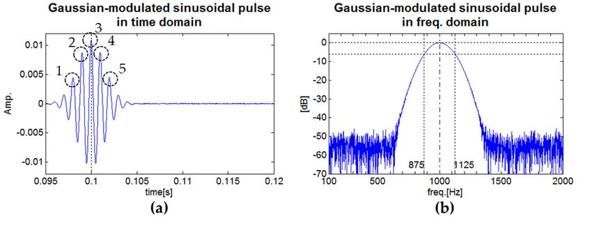
Appl. Sci. 2020, 10, 9090 6 of 25
where P k θ is the power value of the classical SRP, θ is the steered angle, θˆ s is the look direction,
s m is the microphone signal, τˆ m is the delay of each microphone, Wm is the weight, M is the
number of microphones, m is the microphone index, k is the block index, and T is the length of some
finite‐length block signals.
Equations (5) and (6) are the classical SRP using a microphone array, Equation (5) indicates the
integrated output of the steered beamformer, and Equation (6) indicates the direction of the sound source.
The proposed active localization estimates the position of a silent person as an angle and a
distance in the horizontal plane of a linear microphone array (Figure 3). In other words, the proposed
algorithm should represent a two‐dimensional plane. In [34,35], the generalized cross‐correlation–
phase transform (GCC–PHAT) was used to represent the spatial energy map. However, since the
PHAT method revealed that the sound source can be determined well under low noise [36], the
localization performance in the two dimensions is not robust. The proposed algorithm uses the
reflection to estimate the position; thus, the signal‐to‐noise ratio (SNR) is not high. Therefore, the
energy map is expressed by applying the delay and sum beamformer to the classical SRP and a
moving average to the power of the steered block signal. Accordingly, Equations (5) and (6) are
modified as Equations (7) and (9) to represent the energy map on the horizontal plane of the linear
microphone array.
Figure 3. Example of an application of the proposed active localization method to a room.
NL ‐1 M 2
rmeffect t ‐ nL ‐ τˆ m θd
1
P t,θd
NL
wl
nL =0 m=1
t tref , tref 1,, t ref T 1 (7)
,
P tˆ s , θˆ s a rg m a x P t, θ d
t,θ d
(8)
rˆs
tˆ s
tref c
(9)
2 fs
where P t, θd is the energy map of the SRP, θd is the set of desired angles, NL is the length of the
moving average, P ˆt s , θˆ s denotes the position results, tˆ s is the index of the reflected time
sample, rˆ s is the estimated distance between the maximum point and the origin, t ref is the
index of the peak point generated signal (the origin), θˆ s is the estimated angle, c is the speed
of sound, and fs is the sampling frequency.
Figure 4 shows the measured signals of the A position in the experimental configuration when
the boundary absorption coefficient of a room is equal to 0.625. In Equation (7), the length of the block
signals (T) is set as the maximum distance that the signal can reciprocate in the target room. The
estimated distance of an intruder is calculated using Equation (9) through the time information
corresponding to the peak of the sound field variation.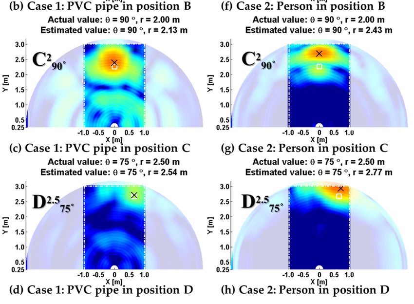
Appl. Sci. 2020, 10, 9090                                                                                   7 of 25

      Figure 4. Example of measured signals: (a) Reference signals before intrusion; (b) event signals after
      intrusion; (c) sound field variation.

      In this study, the input value of the SRP used the changed signal between the reference signal
and the measured signal. In other words, the impulse response in Equation (3) was not directly
predicted, but the sound field variation in the same reproduction signal was estimated by subtracting
the reference signal from the measured microphone signal. We used a triangular moving average of
36 samples in the 48 kHz sampling rate, and the estimated distance was calculated as the product of
time and sound speed. This averaging method empirically reduced the error variance of the
estimated angle and distance in the proposed active localization.
      Figure 5 shows the block diagram used to implement the proposed method using the sound field
variation and the SRP with a moving average. Figure 5a shows the steps to synchronize the measured
signals. Figure 5b shows that the measured signals are stored as the reference signals if no event is
detected, as depicted in Figure 5c, and Figure 5d indicates the proposed SRP to estimate the position of
a silent person.

      Figure 5. Block diagram of the proposed active localization method: (a) Step to synchronize the
      measure signals; (b) Step for reference signals defined as measured signals if no event is detected; (c)
      Step for event detection; (d) Step for SRP using Equations (7)–(9).

     In the signal synchronization step in Figure 5a, we set up the block diagram to minimize the
time delay between the reference signal and event signal for each microphone. Thus, two steps were
involved. The first was to reduce the quantization error by setting the clocks of the loudspeaker and
microphone board identically in hardware. The second step, after measurement, was to verify and
compensate for the time delay between           t ref of Equation (7) and the peak of the generated signal
based on correlation. The event detection in Figure 5c was used to determine intrusion by selecting the
threshold of sound field variation in [17]. In this study, we focused on the analysis of the SRP results in
Figure 5d. In other words, we aimed to analyze the relationship between the variables (reverberation
time and early decay time) in the control space and the signal processing results.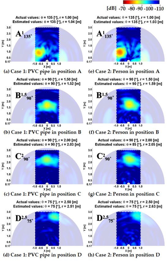
Appl. Sci. 2020, 10, 9090 8 of 25
The signal generated by the loudspeaker formed a sound field with a specific frequency band in a
security area using the Gaussian‐modulated sinusoidal pulse of Equation (10), and then the change
to the sound field was measured using the microphone array.
x t = Ae cos 2πfcenter t ‐ d
‐κ t ‐d
2
(10)
where A is the magnitude of the signal, κ = 5π b fcenter q ln(10) is the envelope constant, b is the
2 2 2
normalized bandwidth, q is the attenuation of the signal, fcenter is the center frequency, and d is the
time delay.
In this study, the center frequency was fixed at 1 kHz, and the attenuation and normalized
bandwidth of the sound source were set to 6 and 0.25, respectively.
The center frequency was 1 kHz because the directivity pattern of the loudspeaker used in the
experiment was cardioid at 1 kHz.
When analyzing a short‐period pure‐tone signal as a frequency component, a discrete‐time
Fourier transform was used, and at least five periods were required to estimate the frequency
components. Therefore, the attenuation and normalized bandwidth were selected to form five
periods in the pulse sound (Figure 6).
Figure 6. Gaussian‐modulated sinusoidal pulse: (a) in the time domain; (b) in the frequency domain.
2.3. Configuration for the Simulations and Experiments
This section describes the configuration of the simulations and experiments. The configuration
shown in Figure 7 was applied to the conceptual verification in an anechoic chamber described in
Section 2.4, the analysis of operating conditions described in Section 3, and the experimental
verification of the proposed method in a classroom described in Section 4.
In Figure 7, A, B, C, and D denote the positions of a silent intruder. Two types of intruders were
used in the experiments in an anechoic chamber and a classroom. The first was a PVC pipe 0.3 m in
diameter. The second was a person.
The reasons for using two types of intruders were as follows. The PVC pipe was used to identify
trends in the localization performance of the proposed active localization method. In other words, using
the circular PVC pipe, the reflection sound was uniformly generated even when the sound source was
incident at any angle. Therefore, the PVC pipe was used to minimize the change in the absorption ratio of
the intruder. The analysis using a PVC pipe was compared with the experimental results of human
intrusion and was the background used to simulate the person as a circular boundary.
Each superscript on the characters A, B, C, and D of the intruder shows the distance between the
active localization system and the intruder position, and each subscript shows the counterclockwise
angle between the microphone array and the intruder. The active localization system consisted of a
loudspeaker, microphone array, and controller. The positions of the silent intruder were represented
by the distance and angle, and the positions of the silent intruder were determined to be the event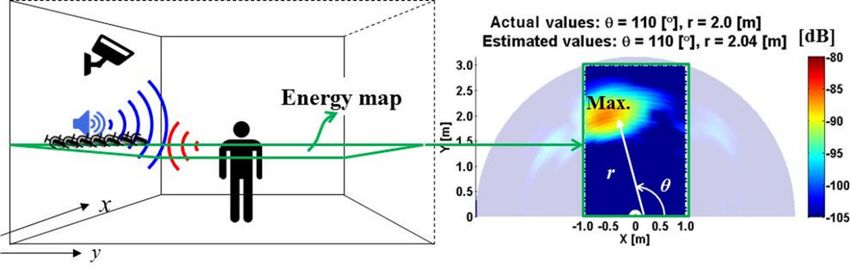
Appl. Sci. 2020, 10, 9090                                                                            9 of 25

scenarios close to the wall (positions A and D) or the center of the active localization system (positions
B and C).

      Figure 7. Experimental configuration for the verification of the proposed approach in terms of
      localization performance using a polyvinyl chloride (PVC) pipe or a human intruder in an anechoic
      chamber or a classroom. A, B, C, and D are the positions of the silent intruder. The superscripts
      represent the distance and the subscripts describe the angle (measured counterclockwise) between
      the microphone array and the intruder.

     The size of the control area in the security zone was 2 m × 3 m. The microphones used in the
experiment were seven‐array microphones. The excitation signal in the simulations and experiments
was a Gaussian‐modulated sinusoidal pulse with a 1 kHz center frequency (Equation (10)) and the
spacing between the microphones was configured to be the same as the Nyquist spacing ( λ 2 ), which
corresponded to a center frequency of 1 kHz. This was because when designing the beamformer of the
single frequency, the Nyquist spacing had the maximum array gain and directivity [37].

2.4. Preliminary Experiments in Ideal Conditions
     This section presents the experimental results in an anechoic chamber. If the proposed method
is directly applied in an actual space, exactly matching the analysis with the experimental results
                                                             effect
becomes difficult because of the various spatial effects ( Rm ). Therefore, the experimental procedure
was performed in an anechoic space to quantitatively verify the accuracy of the proposed approach.
In other words, we excluded the environmental elements of the control space and confirmed that the
proposed concept exhibited no problem under ideal conditions.
     Figure 8 depicts the proposed SRP results obtained from the experiment when a PVC pipe or a
person is a silent intruder. Each image shows the intruder position using relative power values (dB).
     In Case 1 (Figure 8a–d), when examining the position estimation of the intruder (i.e., a PVC
pipe), although the angle had no error, the error of the distance was observed to reach up to 0.04 m
(for position A).
     In Case 2 (Figure 8e–h), the error for the angle was confirmed to reach 5° (for position C) and the
error for the distance ranged up to 0.13 m (position D) if a person was in each intrusion position.
According to these results, when reviewing the energy maps again in terms of the maximum error,
Case 1 indicated that the intruder position was estimated with a relatively small error. This was
because the PVC pipe had a specific boundary condition at a fixed location without moving. As a
result, a consistent reflection wave was measured by the active localization system. However, Case 2
indicated that the reflected signals measured by the microphone array were not constant when a
person was in the intruder position. The reason was that a slight movement occurred although the
person remained in the same position. From this difference, the position estimations of the intruder
in the two cases had different results in terms of the maximum error. Nonetheless, we confirmed the
feasibility of position estimation through reflections.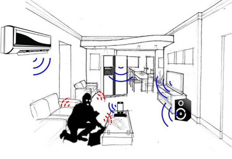
Appl. Sci. 2020, 10, 9090                                                                                    10 of 25

     Two important conclusions can be drawn. Firstly, the position of a person can be detected using
the proposed active localization. Secondly, the energy maps of a person are similar to those of a PVC
pipe, which is a circular object. The result indicates that the active localization method can detect the
position of an object or a person, and it was the basis for modeling a person as a circular object in the
subsequent simulation.

      Figure 8. Energy maps of Case 1 and Case 2 for verification of the localization performance in an
      anechoic chamber: The Case 1 of a PVC pipe in (a) position A; (b) position B; (c) position C; (d) position
      D; Case 2 of a person in (e) position A; (f) position B; (g) position C; (h) position D.
Appl. Sci. 2020, 10, 9090 11 of 25
3. Sound Field Simulation and Its Analysis Using Acoustic Parameters
3.1. Simulation Test for the Reverberant Environment
The active localization method uses reflected sounds; thus, the proposed method is affected by
the boundary condition (the property of the wall surface) of the control space. Consequently, the
error in Equation (3) increases as the reflection on the wall increases, and the detection performance
may be degraded depending on the characteristics of the boundary.
We simulated the environmental operating conditions of the proposed method using the
following steps.
STEP 1: The error of localization performance was analyzed by changing the absorption coefficient
at the boundary of the target control space (2 m × 3 m).
STEP 2: To examine the correlation between the absorption coefficient of the boundary and the spatial
effects, we analyzed the acoustic parameters of the reverberation time (RT20) and early decay time
(EDT).
STEP 3: The operating conditions of the active localization were presented using RT20 and EDT.
The experimental approach makes determining sufficient conditions for the proposed method
difficult. The results of step 1 based on the finite‐difference time‐domain (FDTD) simulation are
presented in Section 3.1.2, and the results of steps 2 and 3 are described in Section 3.2.
3.1.1. Simulation Setup
The FDTD method is the numerical solution of the differential equation of a wave. The FDTD
method is commonly used for nonstaggered compact schemes expressing only pressure [38] and
Yee’s staggered schemes expressing particle velocity and pressure [39].
In this study, the simulation was modeled as Yee’s scheme to use a circular rigid body [40] and
a perfectly matched layer (PML) boundary [41]. The circular rigid body boundary was used to model
the silent intruder because the characteristics of a person and a PVC pipe were observed to be similar.
The PML condition was used to describe the anechoic environment.
The reverberation of the control space was controlled by adjusting the sound absorption
coefficient at the boundary. Hence, the momentum equation with the impedance boundary condition
was used, and it is expressed as follows:
1‐ λc ζ [n‐0.5] 2λc
v[n+0.5] u + 0.5, w = vx u + 0.5, w + p[n] (u, w) (11)
0 c
x
1 + λ c
ζ c 1 + λ ζ
1‐ λ ζ 2λc
v[n+0.5] u ‐ 0.5,w = c v[n‐0.5] u ‐ 0.5,w p[n] (u,w) (12)
0 c
x x
1 + λ c
ζ c 1+ λ ζ
1‐ λ ζ 2λc
v[n+0.5] u,w + 0.5 = c v[n‐0.5] u,w + 0.5 + p[n] (u,w) (13)
y
1 + λ c
ζ
y
0 c 1 + λ c ζ
1‐ λ ζ 2λc
v[n+0.5] u,w ‐ 0.5 = c v[n‐0.5] u,w ‐ 0.5 p[n] (u,w) (14)
y
1 + λ c
ζ
y
0 c 1 + λ c ζ
1 1-α
ζ= (15)
1- 1-α
where p is the sound pressure; vx and vy are the particle velocities of the x and y axes, respectively;
0 is the air density; c is the speed of sound; λ c is the courant number; ζ is the specific acoustic
impedance; α is the absorption coefficient; n is the time index; and u and w are indices of the spatial
point.Appl. Sci. 2020, 10, 9090 12 of 25
In this study, this impedance boundary condition was derived by combining the asymmetric
finite‐difference approximation used in [39] and the locally reacting boundary used in a room
simulation in [38]. The derivation is described in Appendix A. Therefore, we enabled the simulation
of the reverberation environment in the Yee scheme using the change in α.
The FDTD simulation utilized a 2 m × 3 m control space (Figure 7) and a spatial resolution of
0.01 m. The sampling frequency ( fs,FDTD ) was 49 kHz. As the selection criteria of the parameters, a
sampling rate that satisfied the courant condition was selected while the spatial resolution was fixed.
The position of the silent intruder was set at representative positions (A, B, C, and D) as mentioned
in Section 2.3.
The source model in the FDTD simulation is a physically constrained source (PCS) [42], and the
formula is as follows:
0c2 A s
p[n +1] (u, w) = p[n] (u, w) + q [n] (u, w) (16)
fs,FDTD δs
p hm
q[n] (u, w) = s[n] [n]
(17)
ωc if n = 0
s[n]
p =
2Np ‐ 1 !!2 sin nωc
otherwise
(18)
ˆ
bn
2N p + n ‐ 1 !! 2N p ‐
n ‐ 1 !!
b 0 + b 2 e ‐j2ωn
H m e jωn = 1 + a 1 e ‐jωn + a 2 e ‐j2ωn
(19)
[n] 2
where p (u,w) is the pressure node of the source, δs is the spatial resolution, As = 4πa 0 is the
[n]
surface area of the sphere in volume velocity, q (u,w) is the velocity source, s [n]
p is the maximally
flat finite impulse response (FIR) filter, h[n]
m is the mechanical filter of the source represented by a
second‐order infinite impulse response (IIR) filter, H m e jωn is hm in the frequency domain,
[n]
b0 = β M m β2 + R mβ + K m and b2 = ‐b0 are the feedforward filter coefficients,
a1 = 2 K m ‐ M mβ 2 M m β 2 + R mβ + K m and a2 = 1 ‐ 2R m β M m β2 + R mβ + K m are the
feedback filter coefficients, β = ω0 tan ω0 2 is the bilinear operator, and (∗) denotes the
convolution. Mm, Rm = Mm ω0 Q , Km = Mm ω02 , and Q are the mass, damping, elasticity, and
quality factor constants characterizing the mechanical system of the source, respectively. ω0 is the
normalized low resonance frequency of the mechanical system, Mp = 4Np ‐ 1 is the FIR filter order,
and ωc is the normalized cutoff frequency of the FIR filter.
In this study, M p was 16 samples, the normalized cutoff frequency was 0.05, the low resonance
frequency was 300 Hz, Mm was 0.025 Kg, and Q was set to 0.6.
3.1.2. Simulation Results and Analysis
Figure 9 shows the result images of the active localization method by changing the absorption
coefficient of the boundary at position B. The images on the left in Figure 9 show the captured images
in the FDTD simulation obtained by reproducing the PCS model. The images on the right indicate
the energy maps expressed by the convolution signal of Equation (10) and the impulse response
obtained by the FDTD simulation, respectively.Appl. Sci. 2020, 10, 9090 13 of 25
Figure 9. Simulation results of the active localization method according to the change in absorption
coefficient α: (a) α = 0.9; (b) α = 0.7; (c) α = 0.5; (d) α = 0.3. The square marker is the actual position and
the cross marker is the estimated position.
In Figure 9, the reflections propagating from the intruder to the microphone array according to
each alpha are similar. The image results show that the magnitude of the wavefront formed by the
edge boundary increases as the absorption coefficient of the edge boundary decreases. As a result,
the overlap of the reflection formed behind the intruder also increases. In other words, as the reflected
sound formed at the boundary becomes significantly louder than the reflected sound produced by
the intruder, the spatial effect increases such that the overlapped signal is larger than the intruder’s
signal. Therefore, the simulation indicated that the error of position estimation increases with theAppl. Sci. 2020, 10, 9090 14 of 25
boundary characteristics of the control space. The simulation results are summarized in Table 1, in
which the errors in parentheses represent the angular and distance errors.
Table 1. Localization performance of the active localization method according to sound absorption at
the boundary. The errors in parentheses represent the angular and distance errors.
A B C D
135° 1m 90° 1.5 m 90° 2m 75° 2.5 m
135 1.06 90 1.56 90 2.06 75 2.55
PML
(Δθ = 0°) (re = 6%) (Δθ = 0°) (re = 4%) (Δθ = 0°) (re = 3%) (Δθ = 0°) (re = 2%)
135 1.07 90 1.48 90 1.98 75 2.47
α = 0.9
(Δθ = 0°) (re = 7%) (Δθ = 0°) (re = 1.3%) (Δθ = 0°) (re = 1%) (Δθ = 0°) (re = 1.2%)
135 1.16 90 1.48 90 1.98 75 2.47
α = 0.8
(Δθ = 0°) (re = 16%) (Δθ = 0°) (re = 1.3%) (Δθ = 0°) (re = 1%) (Δθ = 0°) (re = 1.2%)
135 1.16 90 1.48 90 2.38 75 2.38
α = 0.7
(Δθ = 0°) (re = 16%) (Δθ = 0°) (re = 1.3%) (Δθ = 0°) (re = 19%) (Δθ = 0°) (re = 4.8%)
135 1.24 90 1.48 90 2.38 75 2.38
α = 0.6
(Δθ = 0°) (re = 24%) (Δθ = 0°) (re = 1.3%) (Δθ = 0°) (re = 19%) (Δθ = 0°) (re = 4.8%)
135 1.24 90 2.12 90 2.38 75 2.84
α = 0.5
(Δθ = 0°) (re = 24%) (Δθ = 0°) (re = 41.3%) (Δθ = 0°) (re = 19%) (Δθ = 0°) (re = 13.6%)
135 1.24 90 2.04 90 2.39 70 2.91
α = 0.4
(Δθ = 0°) (re = 24%) (Δθ = 0°) (re = 36%) (Δθ = 0°) (re = 19.5%) (Δθ = 5°) (re = 16.4%)
135 1.24 90 2.04 90 2.30 70 2.91
α = 0.3
(Δθ = 0°) (re = 24%) (Δθ = 0°) (re = 36%) (Δθ = 0°) (re = 15%) (Δθ = 5°) (re = 16.4%)
As Table 1 shows, the distance error was affected more by the reflectance of the boundary than
by the angular error. There was a 5° error only at the angle at which the sound absorption was below
40% (α × 100%) at the D position. From a distance error point of view, some scenarios failed to detect
an intruder. In other words, when the diameter (0.3 m) of the circle considered as the intruder and
the predicted distance were combined, the estimated distance exceeded the control space of 2 m × 3
m. The results of α being less than 0.6 at position A and less than 0.5 at position D were the result of
detection failure. In addition, when the distance error was viewed in terms of error magnitude, a
large error of 0.5 m or more, at α < 0.5 at position B was observed.
Therefore, we confirmed through the simulation that the approach proposed in this paper
operates at α ≥ 0.7, for which no angular error exists and the distance error is less than 19%.
In the next section, we describe the relational equation that predicts the environment in which
the active localization method operates through the RT20 and EDT of the acoustic parameters. This
is because verifying the operation of the proposed method based on the boundary reflectance in a
general reverberant environment is very difficult.
3.2. Relationship Analysis of Acoustic Parameters and Absorption Coefficients to Propose Operating
Conditions
In this section, the conditions under which the active localization method operates in a
reverberant space are explained using the relationship between the acoustic parameters and the
absorption coefficient discussed in the previous section.
The proposed approach predicts the position of a silent intruder based on the sound reflected
from the intruder, and this phenomenon occurs within a short time; therefore, the pattern of early
reflection is very important. If the maximum distance of the active localization system is estimated to
be 3 m, the sound source generated by a loudspeaker moves for approximately 17.54 ms when the
round‐trip distance of the sound source is 6 m and the speed of sound is 342 m/s. In other words, the
phenomenon occurring within 18 ms should be analyzed.
Therefore, the EDT and RT20 of the acoustic parameters were used to analyze the control space. EDT
includes the direct sound and early reflections, and RT20 has the smallest energy decay time considered
for the reverberation time indices. EDT and RT20 are expressed in the same equation as follows [43]:Appl. Sci. 2020, 10, 9090 15 of 25
L ( t ) 10 log
t
p 2 dt
(20)
0
p 2 dt
Equation (20) normalizes the signal power, and we can calculate the time when power decreases
from 0 to −10 dB and from −5 to −25 dB through the time variable in the denominator. The time
difference of the former is defined as EDT, and the latter is defined as RT20.
When considering the two indices as the early reflection perspective in the RIR, the EDT can
physically determine if a large amount of early reflection occurs at the measured location after the
direct sound is played. This is because the EDT is the time from the measurement of the direct sound
until the signal with an early reflection decrease of −10 dB. RT20 strictly refers to the time when the
reverberation energy decreases gradually except for the direct sound and strong early reflection.
To analyze the relationship between the absorption coefficient and EDT/RT20, the microphone
was placed at the representative intrusion position shown in Figure 7, and the microphone array
signals were compared with the signals of the microphones distributed in the space.
Figure 10a shows the arrangement of the microphones to confirm the operation of the active
localization method proposed here. The first to seventh microphones were the array of microphones
used in the proposed system, and the eighth to eleventh microphones were placed in the
representative positions A, B, C, and D, respectively.
Figure 10. Configuration of (a) acoustic parameter tests to verify the active localization method
according to the change in absorption coefficient α. (b) Energy decay curve of the ninth microphone.
Figure 10b shows the energy decay curve for the impulse response of the ninth microphone. The
energy decay curve of the ninth microphone did not decrease linearly but in a staircase form. This
was because the space represented in this simulation was not diffuse. In other words, no diffuse‐field
reverberation occurred owing to the small space of the simulation and the proximity of the
loudspeaker and microphone. As a result, the energy decay curve had an approximate exponential
shape of a decay curve, but not the diffuse decay curve (Figure 10b). However, the equation was
considered to be suitable for analyzing the space from a physical perspective to confirm the operating
conditions of the proposed method. This was because the proposed method was analyzed based on a
short time, and the changes in the early reflections were presented by the variation of the EDT and RT20
parameters.
Figure 11 shows the results of EDT and RT20 for each microphone as the sound absorption
coefficient decreased. The main point is whether the numerical values measured at the boundaries of
the control spaces from microphones 1 to 7 and those measured in the control space from
microphones 8 to 11 exhibited a specific trend.Appl. Sci. 2020, 10, 9090 16 of 25
Figure 11. (a) Early decay time and (b) reverberation time according to change in α based on the
finite‐difference time‐domain (FDTD) simulation.
Figure 11b indicates that the result of the fourth microphone, which was located at the same
position as the loudspeaker, was very small compared with the results of other microphones. This
was because the loudspeaker and microphone arrangements were very similar such that the
characteristics of the room were not sufficiently reflected. Therefore, when analyzing the results of
RT20, a criterion for the minimum value to be used for the analysis was necessary.
This criterion was selected as the maximum time for the sound from the loudspeaker to reach
the person and back to the microphone again. This is because we can determine that the direct sound
and strong early reflection are dominant in a microphone signal if the measured time of RT20 is
shorter than the propagation time of the sound source generated by the loudspeaker.
The farthest distance in the configuration of this study was 2.62 m, which was the distance from
microphone 4 to the upper corner (2.92 m) minus the distance of 0.3 m at which a person can stand.
The criterion time can be selected as follows:
2dmax 2 2.62
tc = 100 = 100 = 15.3 ms (21)
c 342
where t c is the criterion time, dmax is the maximum distance of a sound source in the control
domain, and c is the speed of sound.
Therefore, when analyzing RT20, values less than t c were excluded from the analysis.
Figure 12 is a graph showing the minimum, maximum, and median values of EDT and RT20 in
the microphone array and control space according to α. In this scenario, the microphone signal that
did not satisfy t c was excluded from the RT20 analysis. The results of the microphones in the array
and control space are represented by the red dashed and blue solid lines, respectively. The marker
on each graph is the median value, the top line of the deviation is the maximum value, and the bottom
line is the minimum value.
Figure 12. Comparison of analysis results between microphones in the array position (MIC1–MIC7)
and microphones in the spatial position (MIC8–MIC11, positions A, B, C, and D) using the (a) early
decay time and (b) reverberation time.Appl. Sci. 2020, 10, 9090 17 of 25
The EDT results shown in Figure 12a indicate that the median value of the microphones in the
control space was higher than that in the array. However, the deviation confirmed that the EDT
results in the array were large depending on the absorption coefficient.
The RT20 results depicted in Figure 12b indicate that until α = 0.7, the median value of the control
space was larger than that of the array, but from 0.6, the opposite result was observed. The deviation
tended to increase and decrease as α decreased.
Analyzing the values in Figure 12 according to the conclusion in Section 3.1.2 that the proposed
approach operated in an environment with α > 0.7, the following features were obtained. From the
EDT results in Figure 12a, we observed that the maximum values of the array became smaller than
the maximum values of the control space when α was greater than 0.7. When the results of RT20 in
Figure 12b were analyzed as a median value, when alpha is greater than 0.7, the median values of the
array were smaller than those of the control space. The results are summarized in Table 2.
Table 2. Simulation results of acoustic parameters to confirm the operating conditions of the active
localization method.
EDT1 (ms) RT202 (ms)
α Max Value Median Value
In a Linear Array In Control Space In a Linear Array In Control Space
0.9 0.53 3.12 15.57 17.36
0.8 3.10 5.42 16.73 17.66
0.7 6.04 10.75 17.89 21.23
0.6 14.83 12.16 33.34 29.54
0.5 16.53 13.36 34.02 30.33
0.4 17.81 18.44 50.32 43.13
0.3 21.44 24.97 60.53 56.14
1 EDT: Early decay time (EDT) (0 to −10 dB), 2 RT20: Reverberation time (RT20) (−5 to −25 dB).
As the results in Tables 1 and 2 show, the active localization method proposed in this paper can
detect the position of a person and an object under the following conditions:
max. EDTmarray < max. EDTmspatial (22)
m edian RT20 array
m
< m edian RT20 spatial
m
(23)
RT20array > tc
m
spatial (24)
RT20 m > tc
where m is the microphone index and t c is the criterion time.
Equation (22) indicates a condition in which the maximum EDT value of the array is smaller
than that of the control space. Equation (23) indicates that the median value of RT20 in the array is
less than its median value in the control space, where RT20 values above t c are used.
Therefore, we observed that if the microphones are installed in the array and control space, the
acoustic parameters of EDT and RT20 satisfy the conditions of Equations (22) and (23), and the active
localization method can be implemented.Appl. Sci. 2020, 10, 9090 18 of 25
4. Experimental Results of Active Localization in a Reverberant Environment
This section presents the experimental results to verify the proposed method.
In Section 2.4, we confirmed the feasibility of the proposed approach in an anechoic chamber,
that is, the concept of detecting the position of a person or an object through a reflected sound. The
results of an anechoic chamber indicated that there was no error in Equation (3). However, in an
actual space in which reverberation exists, an error occurs in Equation (3). Therefore, the conditions under
which the active localization method can operate in the reverberation space are identified in Section 3.
We used Equations (22) and (23) to predict whether the active localization method would
function in a classroom, and we describe the experimental results using the proposed method to
estimate the position of a PVC pipe and a person.
4.1. Experimental Configuration and Operating Conditions Test
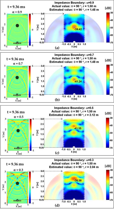
Figure 13 shows the experimental environment of an empty classroom. The experiments were
performed at the same position as the silent intruder (Figure 7). The room acoustic parameters were
measured using the configuration shown in Figure 10a, and the results are presented in Table 3.
Figure 13. Experimental configuration to estimate the position of a PVC pipe using an active
localization system in a classroom. This experiment was performed in an empty classroom to
minimize the influence of the presence of furniture or other interior materials in the room.
Table 3. Results of room acoustic parameters measured in the control space as in Figure 13 at positions
shown in Figure 10a.
Position EDT (ms) RT20 (ms)
1 8.1 24.0
2 2.7 20.0
In a microphone 3 2.0 11.6
array 4 2.0 5
5 2.1 15.5
6 2.6 20.1
7 9.0 23.5
8 (A) 10.5 22.7
In control space 9 (B) 22.8 23.5
10 (C) 13.2 23.6
11 (D) 12.2 25.3Appl. Sci. 2020, 10, 9090 19 of 25
Table 3 shows the EDT and RT20 measured at seven microphones in an array, and the EDT and
RT20 measured at the eighth to eleventh microphones as the representative intrusion shown in
Figures 7 and 10a.
Firstly, when ascertaining the operating conditions using the EDT of Equation (22), the
maximum value measured in the microphone array was 9.0 ms and the maximum value measured
in the control space was 22.8 ms. Therefore, we confirmed that Equation (22) was satisfied.
Secondly, when the operating condition using the median value of RT20 in Equation (23) was
applied to the data in Table 3, the median value of the array was 20.1 ms. By excluding the RT20 that
did not satisfy Equation (24), the median value of the distributed microphones in the control space
was 23.5 ms. Therefore, we confirmed that Equation (23) was also satisfied.
The results indicate that the proposed active localization method operates even if reverberation
exists in the control space set as the security space. The localization results using SRP energy maps
are discussed in the following section.
4.2. Localization Performance in a Reverberant Environment
Figure 14 depicts the energy maps obtained from the experimental results. Case 1 shows the test
results when the PVC pipe was considered as a silent intruder, and Case 2 shows the results when a
person is the silent intruder. Each image shows the intruder position using relative power values
(dB). The square marker is the actual position and the cross marker is the estimated position.
Figure 14. Energy maps of Case 1 and Case 2 to verify the localization performance in a
classroom: The Case 1 of a PVC pipe in (a) position A; (b) position B; (c) position C; (d)
position D; Case 2 of a person in (e) position A; (f) position B; (g) position C; (h) position D.
The square marker is the actual position and the cross marker is the estimated position.Appl. Sci. 2020, 10, 9090 20 of 25
To analyze the experimental results in Figure 14, we compared the estimated position results
with those in Table 1, which lists the simulation results of the reverberation environment. In Table 1,
when examining the results of α greater than 0.7, which is the range in which the active localization
method operates, no error of angle was observed and the error of distance was up to 19% (distance
error 0.38 m).
The experimental results of the reverberation environment in Figure 14 indicate that the angle
had no error, and the error for distance was within 6.5% (distance error 0.13 m). Therefore, the
proposed active localization method can be implemented if the operating conditions of Equations
(22) and (23) are satisfied, as discussed in Section 3.2. However, the position detection results of Case
2 shown in Figure 14 indicate an increased error compared with the results of the PVC pipe. To
analyze this, the results in both an anechoic chamber and a classroom are summarized quantitatively
in Table 4 as the error between the actual and estimated values of each experimental configuration.
These position errors represent angle and distance errors. The results of the localization performances
are compared in terms of the type of silent intruder (a PVC pipe or a person).
Table 4. Position errors of a PVC pipe and a person in terms of localization performance.
PVC pipe Person
Position Anechoic Classroom Anechoic Classroom
Δθ = 0° Δθ = 0° Δθ = 0° Δθ = 0°
A1135 Δr = 0.04 m Δr = 0.06 m Δr = 0.03 m Δr = 0.11 m
(4%) (6%) (3%) (11%)
Δθ = 0° Δθ = 0° Δθ = 0° Δθ = 0°
B1.590 Δr = 0.02 m Δr = 0.03 m Δr = 0.09 m Δr = 0.51 m
(1.33%) (2%) (6%) (34%)
Δθ = 0° Δθ = 0° Δθ = 5° Δθ = 5°
C290 Δr = 0.03 m Δr = 0.13 m Δr = 0.05 m Δr = 0.43 m
(1.5%) (6.5%) (2.5%) (21.5%)
Δθ = 0° Δθ = 0° Δθ = 0° Δθ = 0°
D2.575 Δr = 0.01 m Δr = 0.04 m Δr = 0.13 m Δr = 0.27 m
(0.4%) (1.6%) (5.2%) (10.8%)
The data of the anechoic chamber indicated the initial error of the proposed method under the
condition that no effect of reflection and reverberation occurred in the control space, and the data of
the classroom indicated the performance of the proposed method under conditions of reflection and
reverberation. In an anechoic environment that represented the initial error, the position error
increased in the scenario of a person compared with that of a PVC pipe. This was caused by the slight
movement of the person, and the data results in Table 4 indicate that the position error can be further
increased when this movement is combined with a reverberation environment.
From the experimental results of Case 2 in a classroom, we confirmed that the results of the PVC
pipe had a small error, within 6.5%, owing to the nonmovement of a pipe, whereas the cases of a
human intruder indicated a relatively large error, within 5° of the estimated angle and 34% of the
estimated distance.
Therefore, the above results of localization performance improve the limitations of the existing
acoustic‐based security system, for which an intruder must generate sound. Moreover, the proposed
method estimates the x and y positions using a linear microphone array in a two‐dimensional security
space.
5. Conclusions and Discussion
In this paper, a new active localization method is proposed to estimate the position of a silent
intruder.
For feasibility testing and analysis of the proposed method, we performed the following four
steps. Firstly, feasibility tests were performed in an anechoic chamber. Secondly, an FDTD simulationAppl. Sci. 2020, 10, 9090 21 of 25
was conducted to verify that the proposed method operates according to the reflection in the
boundary of the control space. Thirdly, EDT and RT20 were used to represent the conditions under
which active localization can operate in a reverberant environment through FDTD simulation data.
Finally, the operation of the active localization method in a classroom was confirmed under
conditions based on the EDT and RT20, and then we analyzed the localization results of a PVC pipe
and a person through energy maps. Therefore, the proposed method was verified for the position
estimation of a silent intruder. The active localization method is expected to be applied in home
security systems in conjunction with conventional security sensors to improve the capability of
intrusion detection because the proposed system can estimate the position of a silent intruder and
can be implemented using loudspeakers and microphones built‐in in home appliances.
In a further study, we intend to expand the frequency band to conduct more precise analyses of
the security space, represent the SRP energy maps using wideband data, and design digital filters to
determine the robustness of the proposed method.
Author Contributions: Conceptualization, K.K., S.W, and S.Q.L.; methodology, K.K.; software, K.K.; validation,
K.K., H.R., S.W., and S.Q.L.; formal analysis, K.K.; data curation, K.K., and H.R.; writing—original draft
preparation, K.K.; writing—review and editing, S.W.; supervision, S.W. All authors have read and agreed to the
published version of the manuscript.
Funding: This research was funded by the “GIST Research Institute (GRI)” grant funded by the GIST in 2020.
Conflicts of Interest: The authors declare no conflict of interest.
Appendix A
The simulation was modeled as the Yee scheme of the FDTD method (Figure A1).
Figure A1. Example of a Yee scheme in the finite‐difference time‐domain method.
The wave equation is expressed as a two‐dimensional linear acoustic domain [39].
δt
v [nx + 0.5] u + 0.5, w = v [nx ‐0.5] u + 0.5, w [p[n] (u + 1, w) ‐ p[n] (u, w)] (25)
0 δs
δt
v [ny + 0.5] u, w + 0.5 = v [ny ‐0.5] u, w + 0.5 [p[n] (u, w + 1) ‐ p[n] (u, w)] (26)
0 δs
0 c 2 δt
p[n+1] (u, w) = p[n] (u, w) [v[n+0.5]
x (u + 0.5, w) ‐ v[n+0.5]
x (u ‐ 0.5, w)]
δs
(27)
c 2 δt [n+0.5]
0 [v y (u, w + 0.5) ‐ v[n+0.5]
y (u, w ‐ 0.5)]
δsYou can also read