Facial Landmarks Localization using Cascaded Neural Networks
←
→
Page content transcription
If your browser does not render page correctly, please read the page content below
1
Facial Landmarks Localization using Cascaded Neural Networks
Shahar Mahpoda , Rig Dasb,∗∗, Emanuele Maioranab , Yosi Kellera , Patrizio Campisib
Mahpod & Y. Keller are with the Faculty of Engineering, Bar-Ilan University, Ramat Gan 52900, Israel (e-mail: mahpods@biu.ac.il, yosi.keller@gmail.com)
a S.
Das, E. Maiorana & P. Campisi are with the Section of Applied Electronics, Department of Engineering, Roma Tre University, Via Vito Volterra 62, 00146,
b R.
Rome, Italy (e-mail: {rig.das, emanuele.maiorana, patrizio.campisi}@uniroma3.it)
ABSTRACT
The accurate localization of facial landmarks is at the core of face analysis tasks, such as face recog-
nition and facial expression analysis, to name a few. In this work, we propose a novel localization
approach based on a deep learning architecture that utilizes cascaded subnetworks with convolutional
neural network units. The cascaded units of the first subnetwork estimate heatmap-based encodings of
the landmarks’ locations, while the cascaded units of the second subnetwork receive as input the out-
put of the corresponding heatmap estimation units, and refine them through regression. The proposed
scheme is experimentally shown to compare favorably with contemporary state-of-the-art schemes,
especially when applied to images depicting challenging localization conditions.
c 2021 Elsevier Ltd. All rights reserved.
1. Introduction
The localization of facial landmark points, such as eyebrows,
eyes, nose, mouth, and jawline, is one of the core computational
components in visual face analysis, with applications in face
recognition (Huang et al., 2013), kinship verification (Mahpod
and Keller, 2018), and facial attribute inference (Kumar et al.,
2008), to cite a few. Robust and accurate localization entails
several difficulties, due to variations in face pose, illumination,
(a) (b)
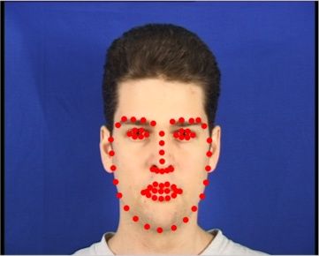
and resolution, as well as to occlusions, as depicted in Figure 1.
Traditional approaches for facial landmark localization have Fig. 1. Facial landmark localization. Each image feature, marked by a
relied on appearance models, providing parametric or non- point, is considered a particular landmark, and is localized individually.
(a) A frontal face image from the XM2VTS datasets (Messer et al., 2003).
parametric descriptors of a face shape. In this context, fit- (b) An image from the Helen dataset (Le et al., 2012) with non-frontal pose
ting strategies have been defined to minimize the residual error and expression variation, making the localization challenging.
between the training face images and their synthesized model
(Cootes and Taylor, 1992).
sion model is iteratively estimated. Besides achieving high lo-
Regression-based approaches have been then successfully
calization accuracy, these schemes are also computationally ef-
proposed, showing improved accuracy compared to their pre-
ficient, commonly requiring less than 1ms processing time per
decessors, especially when applied to in-the-wild face images
frame (Ren et al., 2014). Yet, given that they rely on an initial
(Cao et al., 2012). Starting from an initial estimate of the land-
estimate of the landmarks’ positions, they are in general limited
marks’ positions, typically obtained computing local image fea-
to yaw, pitch, and head roll angles of less than 30◦ , and are thus
tures from an average face template, a high-dimensional regres-
susceptible to initialization and convergence issues. Contempo-
rary approaches might therefore underperform when employed
in challenging conditions (Shao et al., 2017).
∗∗ Please cite this work as: S. Mahpod, R. Das, E. Maiorana, Y. Keller, P.
Campisi, “Facial Landmarks Localization using Cascaded Neural Networks,”
Further improvements in facial landmarks localization have
Computer Vision and Image Understanding, Vol. 205, April 2021. Digital been achieved with the exploitation of deep-learning-based ap-
Object Identifier 10.1016/j.cviu.2021.103171 proaches. In particular, a notable innovation allowed by con-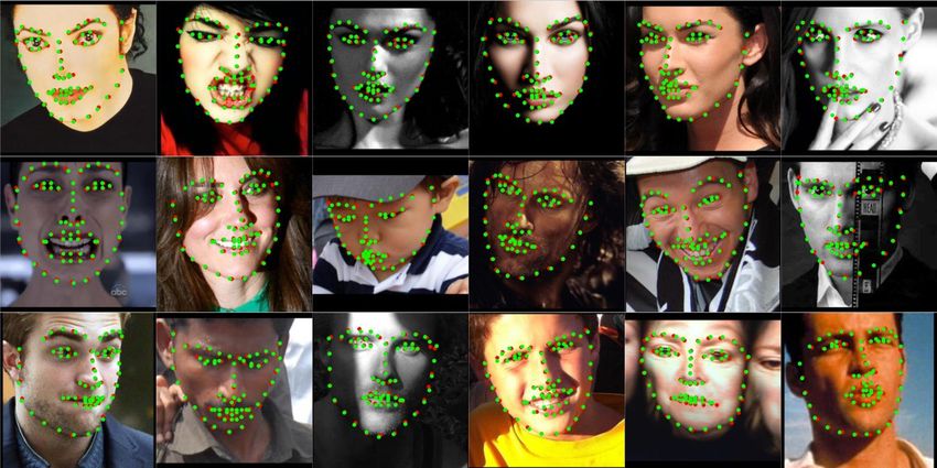
2

                                                                             by cascaded subnetworks, that allow an iterative refine-
                                                                             ment of the localization accuracy. To the best of our
                                                                             knowledge, this is the first such formulation of the face
                                                                             localization problem;
                                                                          • the proposed CCNN framework is experimentally shown
                                                                            to outperform contemporary state-of-the-art approaches.

                                                                           A review of the major contributions in literature regarding
                                                                        facial landmarks localization is provided in Section 2. The
                                                                        proposed CCNN architecture is then detailed in Section 3, and
                                                                        its effectiveness is outlined through the experimental tests dis-
                                                                        cussed in Section 4. Conclusions are finally drawn in Section
                                                                        5.
Fig. 2. Outline of the proposed CCNN framework. The CCNN consists of
base CNNs, preceding the cascaded heatmap subnetwork (CHCNN) esti-      2. State-of-the-Art: Facial Landmark Point Localization
mating the heatmaps, and the cascaded regression CNN (CRCNN) refining
the heatmaps localization via point-wise regression.                       The localization of facial landmark points is a fundamental
                                                                        computer vision task that has been studied in a multitude of
volutional neural networks (CNNs) has consisted in the ame-             works, dating back to the seminal works on active shape mod-
lioration of heatmap-based techniques, following the seminal            els (ASMs) (Cootes and Taylor, 1992), active appearance mod-
work of Pfister et al. (2015). Heatmaps are general-purpose             els (AAMs) (Cootes et al., 2001), and constrained local models
descriptors which can be employed to represent sets of points.          (CLMs) (Cristinacce and Cootes, 2006), which have paved the
Typically, they can be obtained by applying smoothing filters,          way for recent localization schemes. Classical face localiza-
such as diffusion kernels, to characterize a point depending on         tion schemes utilize either parametric (Cristinacce and Cootes,
the geometry of its surroundings (Coifman and Lafon, 2006).             2006) or non-parametric (Belhumeur et al., 2013) models to
Although generating heatmaps through CNNs has guaranteed                learn the statistical distribution of face landmark points, in or-
state-of-the art results in terms of robustness, the achievable lo-     der to provide the actual position of the interested locations in
calization accuracy is inherently limited, due to the coarse spa-       the treated images, trying to deal with significant appearance
tial resolution of the created heatmaps, typically much lower           and pose variations.
than the one of the original image.                                        More recently, state-of-the art results on facial landmarks lo-
   In this work we exploit the upsides of the most com-                 calization have been achieved by resorting to regression- and
monly employed regression- and heatmap-based approaches,                heatmap-based methods, and exploiting deep learning strate-
by proposing a novel deep-learning-based framework for facial           gies to learn high-level facial features. The following subsec-
landmark localization, formulated as a cascaded CNN (CCNN)              tions provide an overview of the most relevant works resorting
comprising two paired cascaded heatmap and regression sub-              to such approaches.
networks. An outline of the architecture of our proposed CCNN
is depicted in Figure 2. In more detail, the cascaded heatmap           2.1. Cascaded Shape Regression Schemes
subnetwork (CHCNN) consists of multiple successive heatmap-                Cascaded Shape Regression (CSR) (Trigeorgis et al., 2016)
based localization units, which perform a robust and coarse             schemes localize landmark points through an iterative process,
localization. The following cascaded regression CNN (CR-                where regression estimates are progressively refined using lo-
CNN) subnetwork refines the heatmap-based localization per-             cal image features, computed at the selected landmarks’ loca-
forming a coarse-to-fine estimate. Cascaded architectures have          tions, as inputs. Such schemes are commonly initialized with
been employed in the proposed subnetwork due to their proven            an estimate of the landmarks based on an average face template,
ability in improving the localization accuracy of regression-           and a bounding box of the face provided by a detector such as
and heatmap-based schemes. The cascaded layers in both the              Viola-Jones (Viola and Jones, 2001). CSR-based approaches
CHCNN and CRCNN are non-weight-sharing, allowing each                   have been shown to be computationally efficient by applying
to separately learn a different localization range. The proposed        fast regression cascades, yet their convergence, and the result-
CCNN is experimentally shown to compare favourably with                 ing localization accuracy, might be susceptible to an inaccurate
contemporary state-of-the-art face localization schemes. Al-            initialization. Actually, as the common initialization of the face
though this work exemplifies the use of the proposed approach           landmarks corresponds to frontal head poses, CSR schemes are
in the localization of facial landmarks, it is of general applica-      typically limited to yaw, pitch, and head roll angles of less than
bility, and can be used for any class of objects.                       30◦ .
   Thus, the contributions of this work are as follows:                    Notable examples of employed local features include scale-
  • we derive a CNN-based face localization scheme using a              invariant feature transform (SIFT) characteristics (Lowe, 2004),
    coarse and robust heatmap estimate, followed by a subse-            used in the supervised descent method (SDM) proposed by
    quent regression-based refinement;                                  Xiong and De la Torre (2013). Local binary features (LBFs)
                                                                        have been instead employed to estimate facial landmarks’ loca-
  • the heatmap estimation and regression tasks are performed           tions through regression trees in Ren et al. (2014), with a low
3

required computational complexity allowing to process images          next step of the regression refinement. A deep alignment net-
at 3000 fps. Computationally efficiency has been also sought in       work (DAN) based on a cascaded CNN, where each stage re-
Chen et al. (2014), where random forests regression has been          fines the landmark positions estimated by the preceding one,
applied to Haar-like local image features.                            has been also presented in (Kowalski et al., 2017). In order to
   An explicit shape regression (ESR) is performed in Cao             extract features from the entire face, instead of relying on local
et al. (2012), where a vectorial regression function inferring the    patches, heatmaps are employed at the initialization stage of the
whole set of facial landmarks is directly learned from the input      DAN method to provide visual information about landmark lo-
image, designing a two-level boosted regression using shape-          cations. A landmark heatmap is an image with high intensity
indexed and correlation-based features. A unified model for           values around the interested landmark locations, and intensity
face detection, pose estimation, and landmark localization has        decreasing proportionally to the distance from the nearest land-
been instead suggested in Zhu and Ramanan (2012). The facial          mark. Differently from the approaches mentioned in the fol-
features and their geometrical relations are there encoded by the     lowing subsections, and also from our approach, the heatmpas
vertices of a graph, while the regression inference is obtained       employed in the DAN method are not estimated through CNNs,
resorting to a mixture of trees, learned using a training set, with   but used solely as a mean for transferring information between
a shared pool of parts. An iterative coarse-to-fine shape search-     stages (Kowalski et al., 2017).
ing (CFSS) refinement method has been introduced in Zhu et al.
(2015), where the initial coarse solution allows to constrain the     2.3. Heatmap-based Schemes
search space of the finer shapes, thus allowing to avoid subop-
                                                                         Exploiting multiple convolution layers and nonlinear ac-
timal local minima, and improving the estimation of large pose
                                                                      tivation functions, deep learning approaches have been also
variations.
                                                                      employed to deal with landmarks localization by creating
2.2. Deep Learning-based Schemes                                      heatmaps significantly different than the ones obtained through
   Deep learning techniques have been applied to face landmark        classical approaches (Coifman and Lafon, 2006), thus provid-
localization in Zhang et al. (2016), where a multi-task estima-       ing the means for achieving high robustness. Facial landmark
tion of facial attributes, such as gender, expression, and ap-        localization and human pose estimation have been first per-
pearance attributes has been performed using a task-constrained       formed resorting to heatmaps and CNNs to detect the Synovial
deep convolutional network (TCDCN), guaranteeing robust and           joints (Pfister et al., 2015), with the optical flow used to fuse
accurate estimates. The authors of Chen et al. (2017) have in-        heatmap predictions from consecutive frames. This approach
stead proposed a 4-stage coarse-to-fine framework (CTFF) for          has been extended (Belagiannis and Zisserman, 2017) by deriv-
landmark localization, with the interested points first coarsely      ing a cascaded heatmap estimation subnetwork, consisting of
predicted, and then refined by extracting multi-scale patches.        multiple heatmap regression units, where the heatmap is esti-
An attention gate network applied to fuse all results.                mated progressively such that each heatmap regression unit is
   A joint usage of deep learning techniques and regression-          given its predecessor’s output. The obtained localization esti-
based schemes has been proposed in Trigeorgis et al. (2016)           mates are characterized by a high robustness. However, their
with the mnemonic descent method (MDM), where feature                 accuracy is inherently limited by the coarse spatial resolution
learned through a CNN are processed through regression, thus          of the generated heatmaps, typically in the order of 1/4th with
yielding an end-to-end trainable scheme.                              respect to the input image. This kind of approach is of particu-
   A framework based on cascaded CNN regressions, which               lar interest in our work, which is based on heatmap estimation
progressively refine localization, has been introduced in Xiao        refined through a cascaded regression subnetwork.
et al. (2016). The landmark locations are there sequentially             A two-stage architecture (TSA), where heatmaps are first es-
improved at each stage, allowing the more reliable ones to be         timated through a basic landmark prediction stage, and then re-
processed earlier. The proposed recurrent attentive-refinement        fined using a whole landmark regression stage made of a set
(RAR) approach uses long short-term memory (LSTM) net-                of shape regression subnetworks, each adapted and trained for
works to identify reliable landmarks, and refine their localiza-      a particular pose, has been proposed in Shao et al. (2017).
tion. Recurrent networks have been also employed in Lai et al.        As the varying appearances of the face images might reduce
(2017), where a deep recurrent regression (DRR) approach has          the localization accuracy, Dong et al. (2018) have proposed a
been designed, by leveraging on deep shape-indexed features           style aggregated network (SAN), that exploits a generative ad-
and recurrent shape features to learn the connections between         versarial network (GAN) to compute an appearance-invariant
the regressions. A sequential linear regression has been used to      face representation. This aggregates varying face appearances,
learn and update the shapes.                                          such as dark and light faces images, and improves the localiza-
   In (He et al., 2017b), the authors have combined cascaded          tion accuracy. A conditional GAN (CGAN) has been instead
shape regression with a CNN, applying a fully end-to-end cas-         employed by Chen et al. (2020) to induce geometric priors on
caded CNN (FEC-CNN) (He et al., 2017a) as a backbone net-             the face landmarks, by introducing a discriminator that classi-
work. Differently from the SDM approach in Xiong and De               fies real vs. erroneous (“fake”) localizations.
la Torre (2013), which learns a cascaded linear regression us-           The aforementioned approaches, representing the state of the
ing projection matrices of SIFT descriptors, the FEC-CNN ap-          art on facial landmark localization using either regression- or
proach extracts differentiable shape-indexed patches, and feeds       heatmap-based methods, are taken into account in Section 4 to
them into the subnetworks to predict the shape residual for the       compare the performance achievable with the proposed frame-
                                                                      work, with the results currently available in literature.
4

                                                                           heatmaps depends on the scale factor s. The cascaded formula-
                                                                           tion implies that the kth heatmap unit (HMU) receives as inputs
                                                                           the heatmap Ĥk−1 estimated by its predecessor, along with the
                                                                           feature map F2 . The HMUs are non-weight-sharing, as each
                                                                           unit refines a different estimate of the heatmaps, thus learning
                                                                           a different regressor. Our scheme therefore differs from the
                                                                           heatmap-based pose estimation of Belagiannis and Zisserman
                                                                           (2017), which employs weight-sharing cascaded units. Each
                                                                           HMU is trained using the loss:

                                                                                                   , s ,N
                                                                                                       w h
                                                                                              s2 sX       h                            i2
                                                                                     LHM   =               Hk (x, y, i) − Ĥk (x, y, i) ,   (1)
                                                                                             whN y,x,i=1

                                                                                           w    h
                                                                           where Hk ∈ R s × s ×N , k = 1, . . . , K, represent the ground-truth
                                                                           heatmaps, derived from the ground-truth set of points P by ap-
                                                                           plying to each landmark a 2D symmetric Gaussian filter with
                                                                           standard deviation σ.
                                                                              The landmark estimates P̂k = {p̂(i)      N
                                                                                                                    k }1 of each HMU are ob-
                                                                           tained as the locations of the maxima of Ĥk , that is, p̂(i)  k =
                                                                           argmax x,y Ĥk (x, y, i). Such points, computed on a coarse grid,
                                                                           are then refined by the third subnetwork, i.e., the cascaded re-
                                                                           gression CNN (CRCNN). This latter consists of K cascaded
                                                                           landmark regression units (LRUs), with the kth LRU receiving
Fig. 3. Outline of the proposed CCNN localization network. The input im-
                                                                           as input the output of its preceding LRU, that is, Ek−1 , the out-
age is encoded by two Base subnetworks, BaseCNN1 and BaseCNN2 . Their
outputs are processed by the Cascaded Heatmap CNN (CHCNN), made of         put Hk of the corresponding HMU, and the outputs of the base
heatmap estimation units (HMUs), and refined by the Cascaded Regres-       subnetworks, namely F1 , F2 , and HE . Each LRU applies a re-
sion CNN (CRCNN), consisting of landmark regression units (LRUs).          gression loss to improve the heatmap-based landmark estimate,
                                                                           by computing the refinement R̂k ,
3. Proposed Face Localization using a Cascaded CNN

   A face landmarks localization task consists in searching for                                    R̂k = vec (P) − vec P̂k ,                (2)
                     n oN
a set of points P = p(i) , such that p(i) =[x(i) , y(i) ]T , in an im-     where vec (·) is a vectorized replica of the N points in a set.
                          1
age I ∈ Rw×h×3 , corresponding to pre-established facial fiducial          Equation 2 is optimized using the landmark loss function
points. The number N of data to be estimated relates to the
                                                                                                             2N
used annotation convention. Figures 2 and 3 depict the general                                          1 X                  2
and detailed architecture of the proposed CCNN, respectively,                                  LLM =          Rk (i) − R̂k (i) ,            (3)
                                                                                                       2N i=1
comprising a total of three sub-networks.
   The heatmap is used as a state variable initiated by the base           where Rk ∈ R2N are the distances (separately for the horizon-
subnetwork (Section 3.1), and is iteratively refined by applying           tal and vertical directions) between the ground-truth landmarks
two complementary losses:                                                  and the estimates computed by the heatmaps.
                                                                              The details of the designed subnetworks are reported in the
  • the heatmap-based loss, (Section 3.2), that induces the
                                                                           following. All convolutional layers of the proposed CCNN are
    graph structure of the detected landmarks, and
                                                                           implemented with a subsequent batch normalization layer.
  • the coordinates-based representation, refined by pointwise             3.1. Base Subnetwork
    regression (Section 3.3).
                                                                               The proposed Base subnetwork consists of two pseudo-
   The first part of our network is a pseudo-siamese (non-                 siamese (non-weight-sharing) units, indicated as BaseCNN1
weight-sharing) sub-network consisting of two subnetworks                  and BaseCNN2 and detailed in Table 1. The input of the net-
{BaseCNN1 , BaseCNN2 }, which compute the corresponding                    work is a face image I ∈ R256×256×3 , having set w = h = 256.
feature maps {F1 , F2 } of the input image, and an initial heatmap             The first part of both BaseCNN1 and BaseCNN2 , comprising
estimate.                                                                  layers A1-A7 from Table 1, computes feature maps from the
   The second subnetwork is a cascaded heatmap CNN                         input image using 3 × 3 filters, and it is indicated as feature map
(CHCNN) that robustly estimates a single 2D heatmap per                    unit (FMU) in Table 1 and Figure 3. The size of the produced
facial feature location. Examples of the generated heatmaps                feature maps is the same as that of the employed heatmaps, and
are depicted in Figure 4. The CHCNN consists of K cas-                     it is set by using s = 4 in the designed architecture. Following
caded heatmap estimation units, each estimating a 3D heatmap               the vast majority of contemporary works on facial landmark
         w h
Ĥk ∈ R s × s ×N , with k = 1, . . . , K. The size of the obtained         localization, and in order to adhere to the 300-W competition
5

Fig. 4. Visualizations of facial landmarks localization heatmaps. The first row shows the face images, while the second row depicts a corresponding single
heatmap of a particular facial feature. The third row shows the corresponding N = 68 points of all heatmap.

Table 1. Base subnetwork architecture. Two such non-weight-sharing units       Table 2. Heatmap estimation unit HMUk , k = 2, . . . , 4. The input to each
are used over here as depicted in Figure 3.                                    HMU is the output of the previous one, combined with the feature map F2 .
                            (a): FMU1 /FMU2                                      Layer                   Feature Map        FSize     Stride      Pad
  Layer                   Feature Map         FSize     Stride     Pad           Input: F2 ⊕ Ĥk−1       64 x 64 x 136        -         -           -
  Input: I                 256 x 256 x 3       -         -          -            B1-Conv                 64 x 64 x 136      7x7        1x1        6x6
  A1-Conv                  256 x 256 x 3      3x3       1x1        2x2           B1-ReLu                  64 x 64 x 64        -         -           -
  A1-ReLu                 256 x 256 x 64       -         -          -            B2-Conv                  64 x 64 x 64     13 x 13     1x1       12 x 12
  A2-Conv                 256 x 256 x 64      3x3       1x1        2x2           B2-ReLu                  64 x 64 x 64        -         -           -
  A2-ReLu                 256 x 256 x 64       -         -          -            B3-Conv                  64 x 64 x 64      1x1        1x1        0x0
  A2-Pool                 256 x 256 x 64      2x2       2x2        0x0           B3-ReLu                 64 x 64 x 128        -         -           -
  A3-Conv                 128 x 128 x 64      3x3       1x1        2x2           B4-Conv                 64 x 64 x 128      1x1        1x1        0x0
  A3-ReLu                 128 x 128 x 64       -         -          -            B4-ReLu                  64 x 64 x 68        -         -           -
  A4-Conv                 128 x 128 x 64      3x3       1x1        2x2
                                                                                 Output: Ĥk              64 x 64 x 68        -         -           -
  A4-ReLu                128 x 128 x 128       -         -          -
  A4-Pool                128 x 128 x 128      2x2       2x2        0x0           LHM regression loss
  A5-Conv                  64 x 64 x 128      3x3       1x1        2x2
  A5-ReLu                  64 x 64 x 128       -         -          -          Table 3. Landmark regression unit LRUk , k = 1, . . . , 4. The input to each
  A6-Conv                  64 x 64 x 128      3x3       1x1        2x2         LRU is the output of the previous one, the output of corresponding HMU,
  A6-ReLu                  64 x 64 x 128       -         -          -          and the feature maps F1 and F2 .
  A7-Conv                  64 x 64 x 128      1x1       1x1         -
                                                                                                              (a): RFMUk
  Output: F1 /F2            64 x 64 x 68       -         -          -
                                                                                  Layer                    Feature Map        FSize     Stride     Pad
                           (b): HMUE /HMU1
                                                                                  Input:
  Layer                   Feature Map         FSize     Stride     Pad            F1 ⊕ F2 ⊕ Ĥk ⊕ HE       64 x 64 x 272       -         -          -
  Input: F1 /F2            64 x 64 x 68        -         -          -             C1-Conv                  64 x 64 x 272      7x7       2x2        5x5
  A8-Conv                  64 x 64 x 68       9x9       1x1        8x8            C1-Pool                   32 x 32 x 64      2x2       1x1        1x1
  A8-ReLu                  64 x 64 x 68        -         -          -             C2-Conv                   32 x 32 x 64      5x5       2x2        3x3
  A9-Conv                 64 x 64 x 128       9x9       1x1        8x8            C2-Pool                  16 x 16 x 128      2x2       1x1        1x1
  A9-ReLu                 64 x 64 x 128        -         -          -             C3-Conv                  16 x 16 x 128      3x3       2x2        1x1
  A10-Conv                64 x 64 x 128       1x1       1x1        0x0            C3-Pool                    8 x 8 x 256      2x2       1x1        1x1
  A10-ReLu                64 x 64 x 256        -         -          -             Output: Ek                8 x 8 x 256        -         -          -
  A11-Conv                64 x 64 x 256       1x1       1x1        0x0
                                                                                                               (b): RLEUk
  A11-ReLu                64 x 64 x 256        -         -          -
  A11-Dropout(0.5)        64 x 64 x 256        -         -          -             Layer                    Feature Map        FSize     Stride     Pad
  A12-Conv                64 x 64 x 256       1x1       1x1        0x0            Input : Ek ⊕ Ek−1        8 x 8 x 512         -         -          -
  A12-ReLu                 64 x 64 x 68        -         -          -             C4-Conv                   8 x 8 x 512       3x3       2x2        1x1
  Output:HE /Ĥ1           64 x 64 x 68        -         -          -             C4-Pool                   4 x 4 x 512       2x2       1x1        1x1
                                                                                  C5-Conv                   4 x 4 x 512       3x3       2x2        1x1
                                                                                  C5-Pool                  2 x 2 x 1024       2x2       1x1        1x1
                                                                                  C6-Conv                  2 x 2 x 1024       1x1       1x1        0x0
guidelines (Trigeorgis et al., 2016; Tuzel et al., 2016), N = 68 is               Output : R̂k             1 x 1 x 136         -         -          -
employed in the designed architecture, thus resulting in feature                  LLM regression loss
maps F1 , F2 ∈ R64×64×68 . The subsequent layers A8-A12 make
up the heatmap units HMUE and HMU1 , which estimate the N                        BaseCNN1 and BaseCNN2 are trained using different losses
heatmaps (one per facial feature) by applying 9 × 9 filters to                 and backpropagation paths, as depicted in Figure 3. Specifi-
encode the relations between neighboring facial features.                      cally, the first Base subnetwork, together with its outputs HE
6

and F1 , is connected to the CRCNN subnetwork, and is there-         (Burgos-Artizzu et al., 2013), a challenging dataset consisting
fore trained by backpropagating its losses LLM . Thus, HE is         of 1, 007 faces depicting a wide range of occlusion patterns.
adapted to the regression task. On the other hand, BaseCNN2          The results obtained on the two considered datasets are respec-
has two outputs, that is, the initial heatmap estimation Ĥ1 and     tively shown in Section 4.1 and 4.2. An ablation study, whose
the feature map F2 , which are forwarded to both the CHCNN           results are outlined in Section 4.3, has been also performed to
and the CRCNN subnetworks, with both the losses LHM and              analyze the specific contribution of each component of the pro-
LLM involved in the backpropagation process.                         posed CCNN architecture.
                                                                        All considered RGB images have been resized to 256 × 256
3.2. Cascaded Heatmap Estimation CNN (CHCNN)
                                                                     pixels, with their values normalized to the range [−0.5, 0.5].
   The heatmaps Ĥk , k = 1, . . . , K, are estimated in a coarse    Training images have been augmented using color variations,
resolution of 1/s, with s = 4, of the input image resolution.        rotation by small angles, scaling, and translations. The learn-
As shown in Figure 3, K = 4 HMUs are employed in the im-             ing rate has been changed gradually, starting with 10−5 for the
plementation of the proposed CCCN localization network. The          initial 30 epochs, followed by 5 × 10⁻⁶ for the following five
structure of the HMUs used in the designed CHCNN is detailed         epochs, and then set to 10−6 for the remaining training epochs.
in Table 2.                                                          The CCNN has been trained for 2,500 epochs in total.
   The cascaded architecture of the CHCNN implies that each             The localization accuracy per single face image has been
HMU estimates a heatmap Ĥk using the heatmap Ĥk−1 received         quantified through the normalized localization error (NLE) be-
from the preceding unit, and the feature map F2 estimated by         tween the localized and ground-truth landmarks, that is,
the base subnetwork BaseCNN2 . Such joint input is shown in
Table 2 as F2 ⊕ Ĥk−1 , with ⊕ denoting the concatenation of vari-                                        N
                                                                                                    1 X (i)
ables along their third dimension. The HMU architecture com-                             NLE =               p̂ − p(i)       2
                                                                                                                                 ,              (4)
                                                                                                   N · d i=1
prises wide filters of sizes [7 × 7] and [13 × 13], corresponding
to the B1-Conv and B2-Conv layers, respectively. These layers        where p̂(i) and p(i) are the estimated and ground-truth coordi-
encode the geometric relationships between relatively distant        nates of a particular facial landmark, respectively. The nor-
landmarks. Each heatmap is trained using LHM (Eq. 1), with           malization factor d is either the inter-ocular distance (the dis-
the locations of the facial landmarks labeled by narrow Gaus-        tance between the outer corners of the eyes) (Ren et al., 2014;
sians with σ = 1.3 to improve training convergence.                  Zafeiriou et al., 2017; Zhu et al., 2015), or the inter-pupil dis-
3.3. Cascaded Regression CNN (CRCNN)                                 tance (the distance between the eye centers) (Trigeorgis et al.,
                                                                     2016).
   The CRCNN is applied to refine the robust, but coarse, land-
                                                                        The localization accuracy for a set of images is quantified
mark estimates of the CHCNN. The CRCNN comprises K = 4
                                                                     by the average localization error and the failures rate. We
LRUs, whose framework is detailed in Table 3. Specifically, the
                                                                     have considered as failures the estimates having a NLE greater
input to the kth regression unit is obtained as the concatenation
                                                                     than α = 0.08 (Trigeorgis et al., 2016). We also report re-
F1 ⊕ F2 ⊕ Ĥk ⊕ HE between the feature maps F1 and F2 com-
                                                                     sults in terms of area under the cumulative error distribution
puted by the base CNNs, the corresponding heatmap estimate
                                                                     curve (AUCα ) (Trigeorgis et al., 2016; Tuzel et al., 2016), sum-
Ĥk , and the activation map HE computed by BaseCNN1 .
                                                                     ming up the obtained error distributions up to α. The pro-
   Specifically, each LRUs consists of two succeeding parts:
                                                                     posed CCNN scheme has been implemented in Matlab and the
  • a regression feature map unit (RFMU), consisting of layers       MatConvNet-1.0-beta23 deep learning framework (Vedaldi and
    C1-C3 in Table 3, which computes the activation map Ek ;         Lenc, 2015) using a NVIDIA Titan XP GPU.

  • a residual localization error unit (RLEU), comprising lay-       4.1. 300-W Results
    ers C4-C6 in Table 3, that estimates the residual localiza-         The 300-W competition dataset comprises images from five
    tion error R̂k .                                                 dabases, namely LFPW, HELEN, AFW, IBUG, and 300-W pri-
   The output of the kth regression unit is the refinement term      vate1 . Each image in the 300-W is annotated with 68 land-
R̂k as in Eq. 2 and Table 3. The network is trained using LLM        marks, and accompanied by a bounding box generated by a face
(Eq. 3), and the final residual localization estimate is given by    detector. In the performed tests, the provided bounding boxes
the last regression unit.                                            have been expanded by 20% on all sides, with the resulting re-
                                                                     gion of interest resized to 256 × 256 pixels.
4. Experimental Results                                                 As in the most established approaches (Kowalski et al.,
                                                                     2017), the available data is divided into training and testing
   The proposed CCNN scheme has been experimentally evalu-           parts (Lee et al., 2015). The former set consists of the AFW
ated on the image datasets typically considered in contemporary      dataset and subsets from the LFPW and HELEN datasets, for a
state-of-the-art works, in order to take into account distinct ap-   total of 3148 images. The proposed CCNN has been trained us-
pearance and acquisition conditions of the considered face im-       ing the 300-W training set, together with the frontal face images
ages. Specifically, we have performed tests on the 300-W com-
petition dataset (Sagonas et al., 2016), a state-of-the-art face
localization dataset comprising 3, 837 near-frontal face images,         1 The “300-W private test set” dataset was originally a private and propri-

and on the Caltech occluded faces in the wild (COFW) dataset         etary dataset used for the evaluation of the 300W challenge submissions.
7
Table 4. Facial landmarks localization results, in terms of NLE (%), on the 300-W common, challenging, LFPW, HELEN, public, and private datasets. Best
results on each dataset are marked in bold.
Inter-ocular normalization Inter-pupil normalization
Category Paper Method
Common Challenging LFPW HELEN Public Private Common Challenging LFPW HELEN Public Private
Ren et al. (2014) LBF - - - - - - 4.95 11.98 - - 6.32 -
CSR Zhu et al. (2015) CFSS - - 5.75 6.35 - 7.51 4.73 9.98 4.87 4.63 5.76 6.27
Kowalski and Naruniec (2016) k-cluster 3.34 6.56 - - 3.97 - - - - - - -
Zhang et al. (2016) TCDCN - - 4.59 4.85 - 3.52 4.80 8.60 6.24 4.60 5.54 10.28
DL
Chen et al. (2017) CTFF - - - - - - 3.73 7.12 - - 4.47 -
Trigeorgis et al. (2016) MDM - - - - 4.05 5.05 - - - - - -
Xiao et al. (2016) RAR - - 3.99 4.30 - - 4.12 8.35 - - 4.94 -
DL+CSR
Lai et al. (2017) DRR - - - - - - 4.07 8.29 4.49 4.02 4.90 -
He et al. (2017b) FEC-CNN - - - - - - 4.98 6.56 - - 5.14 -
Shao et al. (2017) TSA - - - - - - 4.45 8.03 - - 5.15 -
DL+HM Dong et al. (2018) SAN 3.34 6.60 - - 3.98 - - - - - - -
Chen et al. (2020) CGAN - - - - - 3.96 - - - - - -
DAN 3.19 5.24 3.17 3.20 3.59 4.30 4.42 7.57 - - 5.03 -
DL+HM+CSR Kowalski et al. (2017)
DAN-Menpo 3.09 4.88 3.05 3.12 3.44 3.97 4.29 7.05 - - 4.83 -
DL+HM+CSR Proposed approach CCNN 3.23 3.99 3.30 3.20 3.44 3.33 4.55 5.67 4.63 4.51 4.85 4.74
1 1
CFSS CFSS
0.9 TCDCN 0.9 TCDCN
DAN DAN
0.8
Cumulative error distribution
0.8
Cumulative error distribution
DAN-Menpo DAN-Menpo
CCNN CCNN
0.7 0.7
0.6 0.6
0.5 0.5
0.4 0.4
0.3 0.3
0.2 0.2
0.1 0.1
0 0
0 1 2 3 4 5 6 7 8 0 1 2 3 4 5 6 7 8
Normalized localization error (%) Normalized localization error (%)
Fig. 5. CEDs vs. NLE results for the LFPW test set. Fig. 6. CEDs vs. NLE results for the HELEN test set.
Table 5. Facial landmarks localization results, in terms of AUC and failure
from the Menpo dataset (Zafeiriou et al., 2017), also annotated rate (FR, in %) for inter-ocular normalization, on the 300-W public and
with 68 landmark points. The profile faces of the Menpo dataset private datasets. Best results on each dataset are marked in bold.
have been instead annotated with 39 landmark points, and thus Category Paper Method
Public
AUC0.08 FR
Private
AUC0.08 FR
could not have been used in our evaluation. The overall train- Cao et al. (2012) ESR 43.12 10.45 32.35 17.00
CSR Xiong and De la Torre (2013) SDM 42.94 10.89 - -
ing set consists of 11, 007 images, out of which 2, 500 samples Zhu et al. (2015) CFSS 49.87 5.08 39.81 12.30
have been randomly chosen and employed as validation set. DL+CSR Trigeorgis et al. (2016) MDM 52.12 4.21 45.32 6.80
DL+HM Chen et al. (2020) CGAN - - 53.64 2.50
The test data consists of the remaining images from the 300- DL+HM+CSR Kowalski et al. (2017)
DAN
DAN-Menpo
55.33
57.07
1.16
0.58
47.00
50.84
2.67
1.83
W datasets, comprising samples from IBUG, 300-W private, DL+HM+CSR Proposed approach CCNN 57.88 0.58 58.67 0.83
and the test sets from the LFPW and HELEN databases. In or-
der to facilitate comparisons with state-of-the-art methods, the for training, as also done for some tests of the DAN approach
available test data is organized into a common subset, compris- Kowalski et al. (2017), whose results are therefore mentioned
ing test samples from the LFPW and HELEN datasets (554 im- in the following as either DAN or DAN-Menpo, depending on
ages), a challenging subset, given by the IBUG dataset (135 the considered training dataset.
images), a 300-W public subset, consisting of all the test sam- Table 4 reports the NLE performance achieved on the com-
ples from the LFPW, HELEN, and IBUG datasets (689 images), mon and challenging subsets, as well as on the LFPW, HE-
and the 300-W private test set (600 images). LEN, public and private test datasets. The considered state-
In order to evaluate the effectiveness of the proposed ap- of-the-art approaches are grouped into categories relying on
proach, the results achieved with our CCNN architecture are CSR, DL, and HM schemes, as mentioned in Section 2. The
compared with the performance reported in most of the state-of- localization results of the comparison schemes are quoted as
the-art works mentioned in Section 2. All the approaches con- reported in the original papers. The obtained scores testify that
sidered for comparison have been trained on the 300-W train- our CCNN approach compares favorably with respect to all the
ing dataset, while the methods in Chen et al. (2017), He et al. other schemes. In particular, the proposed framework outper-
(2017b), and Shao et al. (2017) have added the Menpo database forms all previous approaches when applied to the challenging
8
1 1
3D Shape Model 3D Shape Model
0.9
0.9
M3CSR M3CSR
CNN Cascade 0.8 CNN Cascade
Cumulative error distribution
0.8
Cumulative error distribution
L norm L2,1 norm
2,1
0.7 Multi-view 0.7 Multi-view
CCNN CCNN
0.6 0.6
0.5 0.5
0.4 0.4
0.3 0.3
0.2 0.2
0.1 0.1
0 0
0 1 2 3 4 5 6 7 8 0 1 2 3 4 5 6 7 8
Normalized localization error (%) Normalized localization error (%)
Fig. 7. CEDs vs. NLE results for the 300-W indoor test set. Fig. 9. CEDs vs. NLE results for the 300-W private test set.
1
3D Shape Model ing well on frontal face images such as those in the HELEN and
0.9 3
M CSR
LFPW datasets, yet tending to fail in challenging conditions
CNN Cascade such as those in the 300-W private set. For instance, applying
0.8
Cumulative error distribution
L2,1 norm the DAN and DAN-Menpo schemes (Kowalski et al., 2017) to
0.7 Multi-view the challenging dataset, mean errors at 5.23% and 4.88% are
0.6
CCNN respectively obtained, whereas our method achieves a smaller
error equal to 3.99%. The ability in producing consistent re-
0.5 sults irrespective of the considered facial conditions is therefore
0.4 a core advantage of the proposed approach over contemporary
state-of-the-art schemes.
0.3 Further results are provided in Table 5, where the AUC0.08
0.2 measures and the localization failure rates of the proposed ap-
proach are compared against state-of-the-art schemes on the
0.1
300-W public and private datasets, for inter-ocular normaliza-
0 tion. The proposed CCNN outperforms all the other schemes
0 1 2 3 4 5 6 7 8
when applied to both test sets.
Normalized localization error (%)
We have also performed tests on the indoor and outdoor sub-
Fig. 8. CEDs vs. NLE results for the 300-W outdoor test set.
sets of the 300-W private test set, as done during the 300-W
challenge (Sagonas et al., 2016). The results obtained in these
set, which comprises face images among the hardest to be pro- scenarios for inter-ocular normalization are reported in terms of
cessed. This capability can be attributed to the use of a combi- CEDs in Figures 7 and 8. The behaviors achieved with state-
nation of cascaded heatmap estimation and regression units. of-the-art approaches are quoted from the results of the 300-W
When applied to the LFPW and HELEN dataset, the pro- challenge2 (Sagonas et al., 2016). Specifically, the 3D Shape
posed CCNN is on par with existing state-of-the-art techniques, Model (Čech et al., 2016), M3 CSR (Deng et al., 2016), CNN
as these datasets mostly consist of easy-to-localize frontal face Cascade (Fan and Zhou, 2016), L2,1 Norm (Martinez and Val-
images. Figures 5 and 6 better detail the observed behaviors, re- star, 2016), and Multi-view (Uřičář et al., 2016) approaches
spectively reporting the cumulative error distributions (CEDs) have been taken into account.
achieved on LFPW and HELEN datasets, when considering The proposed CCNN scheme significantly outperforms all
inter-ocular normalization. contemporary schemes in both indoor and outdoor conditions.
On the other hand, the proposed CCNN outperforms state-of- For the sake of completeness, Figure 9 depicts the CEDs
the-art techniques on the 300-W private dataset, when consider- achieved over the whole 300-W private test set.
ing both the inter-pupil and inter-ocular normalization. The ob- Figure 10 shows some results applying the proposed CCNN
tained results point out that our method is less sensitive to low scheme to images in the 300-W indoor and outdoor test sets.
image quality, larger yaw angles, and facial deformations, with Red and green dots depict the ground-truth and the estimated
respect to the comparison approaches. In fact, a consistent ac-
curacy over all considered image classes is achieved when em-
ploying the proposed CCNN. Conversely, the other approaches 2 https://ibug.doc.ic.ac.uk/media/uploads/competitions/
show notable dependency on the considered scenario, perform- 300w\_results.zip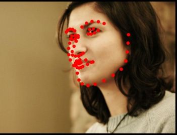
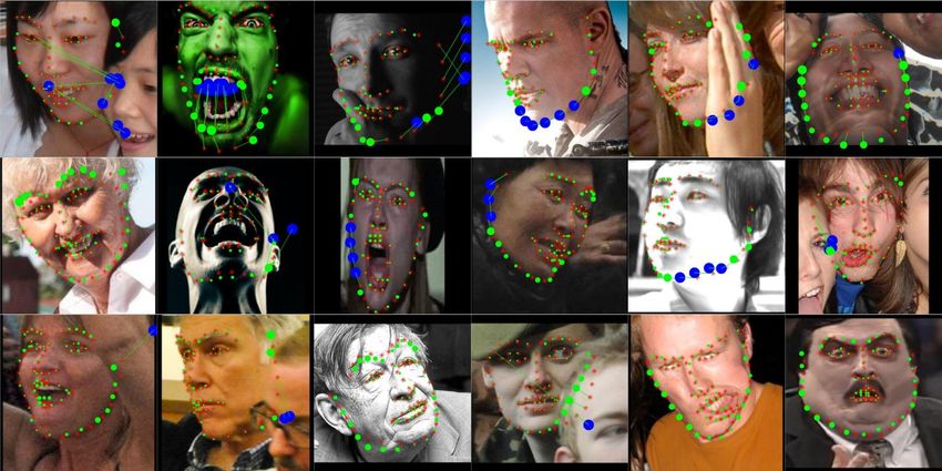
9

Fig. 10. Facial landmarks localization examples, with images taken from the 300-W test set. Red and green dots depict the ground-truth and estimated
landmark points by the proposed CCNN scheme, respectively.

Fig. 11. Facial landmarks localization examples for extremely difficult images, with images taken from the 300-W challenging test set. Red and green dots
depict the ground-truth and estimated landmark points by the proposed CCNN scheme, respectively. The sizes of the green dots increase according to the
error of the estimated landmarks. When the error is more than 20 pixels, a line connects the ground-truth and the estimated landmarks. When the error
is greater than 30 pixels then the landmark point dots are painted in blue.

landmark points, respectively. In particular, we show face im-                 landmarks detected in the 300-W challenging test set. There,
ages with relevant yaw angles, and facial expressions that sig-                the size of green dots increases according to the error of the
nificantly differ from frontal faces. The localization of land-                estimated landmarks. When the error is greater than 20 pixels,
marks on such images exemplifies the effectiveness of the pro-                 a line connecting the ground-truth with the estimated landmarks
posed CCNN framework.                                                          is shown. When the error is greater than 30 pixels, the estimated
   On the other hand, in Figure 11 we report examples of the                   landmark dots are painted in blue.
10
                                 1                                                                             70
                                            CFSS
                                0.9         HPM
                                            RCPR-occ                                                           60
                                0.8
Cumulative error distribution

                                            SAPM
                                0.7         TCDCN                                                              50
                                            SAN
                                0.6         OpenFace

                                                                                                     AUC0.08
                                            CCNN                                                               40
                                0.5
                                                                                                               30
                                0.4

                                0.3                                                                            20                                   300-W Common
                                                                                                                                                    300-W Challenging
                                0.2                                                                                                                 300-W Public
                                                                                                               10
                                0.1                                                                                                                 300-W Private
                                                                                                                                                    COFW
                                 0                                                                              0
                                      0      1       2       3       4       5       6       7   8                  1           2                   3                   4
                                                   Normalized localization error (%)                                          Number of branches (K)

                                          Fig. 12. CEDs vs. NLE results for the COFW test set.       Fig. 13. Ablation study results for the proposed CCNN scheme: perfor-
                                                                                                     mance in terms of AUC0.08 when varying the number of cascades in both
4.2. COFW Results                                                                                    the CHCNN (heatmap) and CRCNN (regression) subnetworks.

   Like the 300-W database, also the COFW dataset has been
                                                                                                     Sections 4.1 and 4.2. The obtained results are depicted in Fig.
annotated with 68 landmark points (Ghiasi and Fowlkes, 2015).
                                                                                                     13 in terms of AUC0.08 , showing that increasing the number
Following the procedure employed in previous works (Burgos-
                                                                                                     of employed cascaded units improves the achievable accuracy.
Artizzu et al., 2013), we have used 500 images for training and
                                                                                                     The most significant improvement is attained when using two
507 for testing the proposed network. The obtained accuracy
                                                                                                     units instead of a single one, with additional cascades providing
has been compared with the publicly available3 performance
                                                                                                     relatively small gains.
achieved with state-of-the-art localization schemes (Ghiasi and
Fowlkes, 2015). In more detail, such results have been obtained                                         Further studies have been conducted to assess the effects
training the CFSS (Zhu et al., 2015) and TCDCN (Zhang et al.,                                        of specific choices in the proposed CCNN design. The ob-
2016) schemes using the HELEN, LFPW, and AFW datasets.                                               tained results are reported in Table 6 in terms of NLE achieved
The RCPR-occ scheme (Burgos-Artizzu et al., 2013) has been                                           over the 300-W Public, 300-W Private, and COFW datasets.
trained using the same training sets as our CCNN model, while                                        As baseline reference, the error rates obtained with the pro-
the HPM, SAPM (Ghiasi and Fowlkes, 2015), SAN4 (Dong                                                 posed CCNN when trained for 2500 epochs, as in the tests de-
et al., 2018), and OpenFace5 (Zadeh et al., 2017) appraches                                          scribed in Section4.1 and 4.2, and for 300 additional epochs,
have been trained using the HELEN and LFPW datasets.                                                 are reported in Table 6, showing that the proposed network has
   The comparative results are depicted in Figure 12 in terms of                                     reached a plateau of performance.
CEDs, showing that the proposed CCNN approach significanlty                                             The usefulness of the CRCNN regression subnetwork in re-
outperforms all the other considered schemes when employed                                           fining the received outputs has been evaluated by performing
on the COFW dataset, furtherly testifying the effectiveness of                                       test relying only on the CHCNN heatmap subnetwork. To do
the proposed method in challenging conditions.                                                       this, the BaseCNN1 and CRCNN subnetworks have been dis-
                                                                                                     connected from the rest of the CCNN network trained for 2800
4.3. Ablation Study                                                                                  epochs, and an additional training has been carried out for a
                                                                                                     further 20 epochs. A performance worsening is observed when
  In order to investigate the contribution of each element in
                                                                                                     carrying out such tests, especially in terms of AUC0.08 .
the proposed CCCN architecture, a detailed ablation study has
been performed focusing on several aspects characterizing the                                           The importance of using two base subnetworks has been in-
proposed approach.                                                                                   vestigated in great detail, by first testing the performance of a
  The influence on the achievable performance of the num-                                            network in which both the F1 and F2 have been disconnected
ber K of cascaded units employed in the CHCNN (heatmaps)                                             from the CRCNN subnetwork. In order to do this, the input
and CRCNN (regression) subnetworks has been first evaluated.                                         layer of LRUs, that is, C1-Conv in Table 3, has been resized and
For this purpose, we have trained the proposed CCNN using                                            re-initialized. As in the previous case, the modified network has
K = {1, 2, 3, 4} cascades, with the same setup and training sets                                     been trained for several additional epochs. The same has been
outlined in Section 4.1, using the same test sets described in                                       done excluding only the F1 feature map from the CRCNN sub-
                                                                                                     network. Furthermore, the whole BaseCNN1 subnetwork has
                                                                                                     been removed from the rest of the architecture, thus letting the
                                3 https://github.com/golnazghiasi/cofw68-benchmark
                                                                                                     landmark regression layers getting their information only from
                                4 https://github.com/D-X-Y/SAN                                       F2 and Ĥk , k = 1, . . . , K.
                                5 https://github.com/TadasBaltrusaitis/OpenFace                         The relevance of the F2 feature map has been instead ad-
11
Table 6. Ablation studies performed on the proposed CCNN architecture. Tests have been done on the 300-W Public, 300-W Private, and COFW datasets.
Results are given in terms of NLE (%), where the best performance marked as bold.
Additional 300-W Public 300-W Private COFW
Tested condition
epochs NLE AUC0.08 NLE AUC0.08 NLE AUC0.08
0 3.44 57.88 3.33 58.67 5.26 39.42
Baseline CCNN
300 3.45 57.03 3.25 59.55 5.23 39.78
CRCNN removed (only CHCNN) 300 + 20 3.47 56.61 3.28 59.28 5.20 39.62
300 + 20 3.57 55.94 3.91 51.96 5.24 40.07
F1 and F2 removed from CRCNN
300+100 3.52 56.02 3.90 51.79 5.10 41.00
300 + 20 3.60 55.78 3.96 51.87 5.29 40.05
F1 removed from CRCNN
300+100 3.54 55.95 3.91 51.70 5.16 40.99
300+20 3.54 55.92 3.90 51.99 5.24 40.43
BaseCNN1 removed
300+100 3.55 55.80 3.93 51.74 5.14 41.14
300+20 3.62 55.54 3.99 51.30 5.27 40.33
F2 removed from CRCNN
300 + 100 3.54 55.94 3.93 51.48 5.13 40.90
300+20 3.45 56.98 3.38 57.86 5.16 40.52
F2 replaced by Ĥk in CRCNN
300+100 3.57 55.73 3.64 55.23 5.68 37.99
300+20 3.69 54.08 3.77 53.49 5.23 39.45
CHCNN and CRCNN with weight sharing
300+100 3.78 53.41 3.94 52.51 5.71 37.98
Only Ĥ4 as input for the CRCNN 300 3.53 55.92 3.91 51.50 5.12 41.08
300+300 3.45 57.02 3.26 59.67 5.13 40.41
K=6 cascaded units in CHCNN and CRCNN
300+500 3.45 57.02 3.27 59.62 5.13 40.44
dressed considering two distinct scenarios: in a first case, F2 an input to the corresponding CRCNN unit. This allows the
is removed as input from the CRCNN subnetwork, and layer iterative refinement of the localization points. The CCNN is
C1-Conv is resized and re-initialized similarly to when F1 is a face localization scheme that is fully data-driven and end-to-
excluded. In a second case, F2 is replaced by Ĥk , k = 1, . . . , K, end trainable. It extends previous results on heatmap-based lo-
as input to each LRUk (with Ĥk therefore included twice in each calization (Belagiannis and Zisserman, 2017), and it is experi-
kth unit), so that C1-Conv can be kept with its original dimen- mentally shown to be robust to large variations in head poses.
sions, without the need for a re-initialization. Moreover, it compares favorably with contemporary face lo-
The need for training the proposed CCNN without resort- calization schemes when evaluated using state-of-the-art face
ing to weight-sharing has been proven by testing a network alignment datasets. The proposed CCNN scheme does not uti-
where units in the CHCNN and CRCNN subnetworks are in- lize any particular appearance attribute of faces, and can be ap-
stead trained to share the same parameters, as in Belagiannis plied to the localization of other classes of objects. Such an
and Zisserman (2017). The results reported in Table 6 testify approach might pave the way for other localization solutions,
that such alternative degrades the achievable accuracy. The bet- such as those dedicated to sensor localization (Gepshtein and
ter behavior of the proposed CCNN is attributed to the capabil- Keller, 2015; Keller and Gur, 2011), where the initial estimate
ity of learning different regression functions per cascade. of the heatmap is given by a graph algorithm, rather than an im-
We have also studied the possibility of using only the output age domain CNN. The succeeding CNN architecture could be
of the CHCNN layer, that is, the highest quality heatmap Ĥ4 , as designed similarly to the proposed CHCNN and CRCNN sub-
input to all the LRUs in the CRCNN subnetwork. The obtained networks, thus offering an opportunity for further extensions in
results show that the proposed CCNN architecture, with paired future works.
HMUs and LRUs, can achieve better performance.
Eventually, we have tested an architecture with two addi- Acknowledgment
tional cascaded units, initialized with the weights from the 4th
cascade, in each of the CHCNN and CRCNN subnetworks. This work has been partially supported by COST Action
A slight improvement has been in this case achieved over the 1206 {“De-identification for privacy protection in multimedia
COFW test set, while the performance on the 300-W dataset content” }. We gratefully acknowledge the support of NVIDIA
has not changed notably. Corporation for providing the Titan X Pascal GPU for this re-
search work.
5. Conclusions
References
In this work, we have introduced a deep-learning-based
cascaded formulation for coarse-to-fine localization of facial Belagiannis, V., Zisserman, A., 2017. Recurrent human pose estimation,
landmarks. The proposed cascaded CNN (CCNN) exploits in: 2017 12th IEEE International Conference on Automatic Face Gesture
Recognition (FG 2017), pp. 468–475. doi:10.1109/FG.2017.64.
two paired cascaded subnetworks: the heatmap subnetwork Belhumeur, P.N., Jacobs, D.W., Kriegman, D.J., Kumar, N., 2013. Localizing
(CHCNN) estimates a coarse but robust heatmap corresponding parts of faces using a consensus of exemplars. IEEE Transactions on Pattern
to the facial landmarks, while the cascaded regression subnet- Analysis and Machine Intelligence 35, 2930–2940. doi:10.1109/TPAMI.
2013.23.
work (CRCNN) refines the accuracy of the CHCNN-generated Burgos-Artizzu, X.P., Perona, P., Dollár, P., 2013. Robust face landmark esti-
landmarks via regression. The two cascaded subnetworks are mation under occlusion, in: 2013 IEEE International Conference on Com-
aligned such that the output of each CHCNN unit is used as puter Vision, pp. 1513–1520. doi:10.1109/ICCV.2013.191.12 Cao, X., Wei, Y., Wen, F., Sun, J., 2012. Face alignment by explicit shape re- Conference on Computer Vision, Florence, Italy, October 7-13, 2012, Pro- gression, in: 2012 IEEE Conference on Computer Vision and Pattern Recog- ceedings, Part III , 679–692doi:10.1007/978-3-642-33712-3_49. nition, pp. 2887–2894. doi:10.1109/CVPR.2012.6248015. Lee, D., Park, H., Yoo, C.D., 2015. Face alignment using cascade gaussian Chen, D., Ren, S., Wei, Y., Cao, X., Sun, J., 2014. Joint cascade face detection process regression trees, in: 2015 IEEE Conference on Computer Vision and and alignment, in: Fleet, D., Pajdla, T., Schiele, B., Tuytelaars, T. (Eds.), Pattern Recognition (CVPR), pp. 4204–4212. doi:10.1109/CVPR.2015. Computer Vision – ECCV 2014, Springer International Publishing, Cham. 7299048. pp. 109–122. Lowe, D.G., 2004. Distinctive image features from scale-invariant keypoints. Chen, X., Zhou, E., Mo, Y., Liu, J., Cao, Z., 2017. Delving deep into coarse- International Journal of Computer Vision 60, 91–110. doi:10.1023/B: to-fine framework for facial landmark localization, in: 2017 IEEE Confer- VISI.0000029664.99615.94. ence on Computer Vision and Pattern Recognition Workshops (CVPRW), Mahpod, S., Keller, Y., 2018. Kinship verification using multiview hybrid dis- pp. 2088–2095. doi:10.1109/CVPRW.2017.260. tance learning. Computer Vision and Image Understanding 167, 28 – 36. Chen, Y., Shen, C., Chen, H., Wei, X., Liu, L., Yang, J., 2020. Adversarial Martinez, B., Valstar, M.F., 2016. L2,1-based regression and prediction ac- learning of structure-aware fully convolutional networks for landmark lo- cumulation across views for robust facial landmark detection. Image and calization. IEEE Transactions on Pattern Analysis and Machine Intelligence Vision Computing 47, 36 – 44. doi:https://doi.org/10.1016/j. 42, 1654–1669. imavis.2015.09.003. Coifman, R.R., Lafon, S., 2006. Diffusion maps. Applied and Computational Messer, K., Kittler, J., Sadeghi, M., Marcel, S., Marcel, C., Bengio, S., Car- Harmonic Analysis 21, 5 – 30. URL: http://www.sciencedirect.com/ dinaux, F., Sanderson, C., Czyz, J., Vandendorpe, L., Srisuk, S., Petrou, M., science/article/pii/S1063520306000546, doi:https://doi.org/ Kurutach, W., Kadyrov, A., Paredes, R., Kepenekci, B., Tek, F.B., Akar, 10.1016/j.acha.2006.04.006. G.B., Deravi, F., Mavity, N., 2003. Face verification competition on the Cootes, T.F., Edwards, G.J., Taylor, C.J., 2001. Active appearance models. xm2vts database. Audio- and Video-Based Biometric Person Authentica- IEEE Transactions on Pattern Analysis and Machine Intelligence 23, 681– tion: 4th International Conference, AVBPA 2003 Guildford, UK, June 9–11, 685. doi:10.1109/34.927467. 2003 Proceedings , 964–974doi:10.1007/3-540-44887-X_112. Cootes, T.F., Taylor, C.J., 1992. Active shape models — ‘smart snakes’, in: Pfister, T., Charles, J., Zisserman, A., 2015. Flowing convnets for human Hogg, D., Boyle, R. (Eds.), BMVC92, Springer London, London. pp. 266– pose estimation in videos, in: International Conference on Computer Vision 275. (ICCV). Cristinacce, D., Cootes, T., 2006. Feature detection and tracking with con- Ren, S., Cao, X., Wei, Y., Sun, J., 2014. Face alignment at 3000 fps via regress- strained local models, in: British Machine Vision Conference, pp. 929–938. ing local binary features, in: 2014 IEEE Conference on Computer Vision Deng, J., Liu, Q., Yang, J., Tao, D., 2016. M3 CSR: multi-view, multi-scale and Pattern Recognition, pp. 1685–1692. doi:10.1109/CVPR.2014.218. and multi-component cascade shape regression. Image Vision Comput. 47, Sagonas, C., Antonakos, E., Tzimiropoulos, G., Zafeiriou, S., Pantic, M., 19–26. doi:10.1016/j.imavis.2015.11.005. 2016. 300 faces in-the-wild challenge: database and results. Image and Vi- Dong, X., Yan, Y., Ouyang, W., Yang, Y., 2018. Style aggregated network sion Computing 47, 3 – 18. doi:https://doi.org/10.1016/j.imavis. for facial landmark detection, in: Proceedings of the IEEE Conference on 2016.01.002. Computer Vision and Pattern Recognition (CVPR), pp. 379–388. Shao, X., Xing, J., Lv, J., Xiao, C., Liu, P., Feng, Y., Cheng, C., 2017. Un- Fan, H., Zhou, E., 2016. Approaching human level facial landmark localiza- constrained face alignment without face detection, in: 2017 IEEE Confer- tion by deep learning. Image Vision Comput. 47, 27–35. doi:10.1016/j. ence on Computer Vision and Pattern Recognition Workshops (CVPRW), imavis.2015.11.004. pp. 2069–2077. doi:10.1109/CVPRW.2017.258. Gepshtein, S., Keller, Y., 2015. Sensor network localization by augmented Trigeorgis, G., Snape, P., Nicolaou, M.A., Antonakos, E., Zafeiriou, S., 2016. dual embedding. IEEE Transactions on Signal Processing 63, 2420–2431. Mnemonic descent method: A recurrent process applied for end-to-end face doi:10.1109/TSP.2015.2411211. alignment, in: 2016 IEEE Conference on Computer Vision and Pattern Ghiasi, G., Fowlkes, C.C., 2015. Occlusion coherence: Detecting and localiz- Recognition (CVPR), pp. 4177–4187. doi:10.1109/CVPR.2016.453. ing occluded faces. arXiv: 1506.08347. URL: https://dblp.org/rec/ Tuzel, O., Marks, T.K., Tambe, S., 2016. Robust face alignment using a mixture bib/journals/corr/GhiasiF15. of invariant experts, in: Leibe, B., Matas, J., Sebe, N., Welling, M. (Eds.), He, Z., Kan, M., Zhang, J., Chen, X., Shan, S., 2017a. A fully end-to-end Computer Vision – ECCV 2016, Springer International Publishing, Cham. cascaded CNN for facial landmark detection, in: 2017 12th IEEE Interna- pp. 825–841. tional Conference on Automatic Face Gesture Recognition (FG 2017), pp. Uřičář, M., Franc, V., Thomas, D., Sugimoto, A., Hlaváč, V., 2016. Multi-view 200–207. doi:10.1109/FG.2017.33. facial landmark detector learned by the Structured Output SVM. Image He, Z., Zhang, J., Kan, M., Shan, S., Chen, X., 2017b. Robust FEC-CNN: and Vision Computing 47, 45 – 59. doi:https://doi.org/10.1016/j. A high accuracy facial landmark detection system, in: 2017 IEEE Confer- imavis.2016.02.004. ence on Computer Vision and Pattern Recognition Workshops (CVPRW), Vedaldi, A., Lenc, K., 2015. Matconvnet – convolutional neural networks for pp. 2044–2050. doi:10.1109/CVPRW.2017.255. matlab, in: Proceeding of the ACM Int. Conf. on Multimedia. Huang, Z., Zhao, X., Shan, S., Wang, R., Chen, X., 2013. Coupling alignments Viola, P., Jones, M., 2001. Rapid object detection using a boosted cascade with recognition for still-to-video face recognition, in: 2013 IEEE Inter- of simple features, in: Proceedings of the 2001 IEEE Computer Society national Conference on Computer Vision, pp. 3296–3303. doi:10.1109/ Conference on Computer Vision and Pattern Recognition. CVPR 2001, pp. ICCV.2013.409. I–511–I–518 vol.1. doi:10.1109/CVPR.2001.990517. Keller, Y., Gur, Y., 2011. A diffusion approach to network localization. IEEE Xiao, S., Feng, J., Xing, J., Lai, H., Yan, S., Kassim, A., 2016. Robust facial Transactions on Signal Processing 59, 2642–2654. landmark detection via recurrent attentive-refinement networks, in: Leibe, Kowalski, M., Naruniec, J., 2016. Face alignment using k-cluster regression B., Matas, J., Sebe, N., Welling, M. (Eds.), Computer Vision – ECCV 2016, forests with weighted splitting. IEEE Signal Processing Letters 23, 1567– Springer International Publishing, Cham. pp. 57–72. 1571. doi:10.1109/LSP.2016.2608139. Xiong, X., De la Torre, F., 2013. Supervised descent method and its applica- Kowalski, M., Naruniec, J., Trzcinski, T., 2017. Deep alignment network: A tions to face alignment, in: 2013 IEEE Conference on Computer Vision and convolutional neural network for robust face alignment, in: 2017 IEEE Con- Pattern Recognition, pp. 532–539. doi:10.1109/CVPR.2013.75. ference on Computer Vision and Pattern Recognition Workshops (CVPRW), Zadeh, A., Baltrusaitis, T., Morency, L., 2017. Convolutional experts con- pp. 2034–2043. doi:10.1109/CVPRW.2017.254. strained local model for facial landmark detection, in: CVPR Workshops, Kumar, N., Belhumeur, P., Nayar, S., 2008. Facetracer: A search engine for IEEE Computer Society. pp. 2051–2059. large collections of images with faces, in: Forsyth, D., Torr, P., Zisser- Zafeiriou, S., Trigeorgis, G., Chrysos, G., Deng, J., Shen, J., 2017. The Menpo man, A. (Eds.), Computer Vision – ECCV 2008, Springer Berlin Heidelberg, facial landmark localisation challenge: A step towards the solution, in: 2017 Berlin, Heidelberg. pp. 340–353. IEEE Conference on Computer Vision and Pattern Recognition Workshops Lai, H., Xiao, S., Pan, Y., Cui, Z., Feng, J., Xu, C., Yin, J., Yan, S., 2017. Deep (CVPRW), pp. 2116–2125. doi:10.1109/CVPRW.2017.263. recurrent regression for facial landmark detection. IEEE Transactions on Zhang, Z., Luo, P., Loy, C.C., Tang, X., 2016. Learning deep representation for Circuits and Systems for Video Technology PP, 1–1. doi:10.1109/TCSVT. face alignment with auxiliary attributes. IEEE Transactions on Pattern Anal- 2016.2645723. ysis and Machine Intelligence 38, 918–930. doi:10.1109/TPAMI.2015. Le, V., Brandt, J., Lin, Z., Bourdev, L., Huang, T.S., 2012. Interactive fa- 2469286. cial feature localization. Computer Vision – ECCV 2012: 12th European
You can also read