A Hypothesis for the Aesthetic Appreciation in Neural Networks

A Hypothesis for the Aesthetic Appreciation
 in Neural Networks

 Xu Cheng Xin Wang
 Shanghai Jiao Tong University Shanghai Jiao Tong University
 xcheng8@sjtu.edu.cn xin.wang@sjtu.edu.cn
arXiv:2108.02646v1 [cs.LG] 31 Jul 2021

 Haotian Xue Zhengyang Liang Quanshi Zhang∗
 Shanghai Jiao Tong University Tongji University Shanghai Jiao Tong University
 xavihart@sjtu.edu.cn marxas@tongji.edu.cn zqs1022@sjtu.edu.cn

 Abstract
 This paper proposes a hypothesis for the aesthetic appreciation that aesthetic im-
 ages make a neural network strengthen salient concepts and discard inessential
 concepts. In order to verify this hypothesis, we use multi-variate interactions to
 represent salient concepts and inessential concepts contained in images. Further-
 more, we design a set of operations to revise images towards more beautiful ones.
 In experiments, we find that the revised images are more aesthetic than the original
 ones to some extent. The code will be released when the paper is accepted.

 1 Introduction
 The aesthetic appreciation is a high-level and complex issue, which influences choices of human
 activities, such as the mate selection, art appreciation, and possibly even the moral judgment. From
 the neurobiological perspective, aesthetic experiences likely emerge from the interaction between the
 emotion–valuation, sensory–motor, and meaning–knowledge neural systems [11, 57].
 Unlike previous studies of aesthetics [12, 14, 17, 46, 50] learning a model to mimic human annotations
 of aesthetic levels in a supervised manner, we consider the aesthetic appreciation inherently rooted
 in the brain. Specially, we roughly classify the aesthetic appreciation into two types, in terms of
 whether the aesthetic appreciation has a direct evolutionary utility or not. Specifically, the aesthetic
 appreciation with a direct evolutionary utility is mainly concerned with the survival and reproduction.
 For example, the physical attractiveness, including the facial beauty, has a direct evolutionary utility
 in the partner selection and may reflect the fertility, gene quality, and health [31]. Whereas, the
 aesthetic appreciation without a direct evolutionary utility can be regarded as a special case of
 cognition, which may reduce cognitive costs of humans. For example, orderly and simple objects
 may appear to be more beautiful than chaotic or complex objects [3].
 Considering the aesthetic appreciation relating to the survival and reproduction is hard to define, in this
 study, we focus on the second type of the aesthetic appreciation without a direct evolutionary utility.
 Specifically, we propose a hypothesis for the aesthetic appreciation that aesthetic images make the
 brain discard inessential “concepts” and enhance salient “concepts”, i.e. triggering clean and
 strong signals to the brain. Note that the concept here is referred to as features for certain shapes
 or textures, instead of representing semantics. For example, when we enjoy a piece of melodious
 music, the Beta wave (a neural oscillation in the brain) may dominate our consciousness, make us
 ∗
 This research is done under the supervision of Dr. Quanshi Zhang. He is with the John Hopcroft Center
 and the MoE Key Lab of Artificial Intelligence, AI Institute, at the Shanghai Jiao Tong University, China.
 Correspondence to: Quanshi Zhang .

 Preprint. Under review.

concentrate, feel excited, and remain in a state of high cognitive functioning [7, 1, 5]. Moreover,
based on the hypothesis, we develop a method to revise images towards the more beautiful ones.
However, this hypothesis is difficult to be formulated and to be used to handle images, from the
neurobiological perspective. It still remains a challenge to find a convincing and rigorous way of
disentangling inessential concepts away from salient concepts encoded by biological neural networks.
Hence, we use an artificial deep neural network (DNN) learned for object classification on a huge
dataset (e.g. the ImageNet dataset [39]) as a substitute for the biological neural network. Given a
pre-trained DNN f and an image with n pixels N = {1, 2, . . . , n}, we use a metric in game theory,
namely the multi-variate interaction, to distinguish inessential concepts and essential salient concepts
encoded in the intermediate layer of the DNN. Based on the multi-variate interaction, we further
revise the image to ensure that the DNN discards inessential concepts and strengthens essential salient
concepts. Therefore, we can verify the hypothesis for the aesthetic appreciation by checking whether
the revised images look more beautiful or not.
To this end, we consider a group of highly interacted pixels as a certain visual concept. The multi-
variate interaction between multiple pixels is defined in game theory, which measures the marginal
benefit to the network output when these pixels collaborate w.r.t. they work independently. As a toy
example, the nose, mouth, and eyes have a strong interaction in the prediction of the face detection,
because they collaborate with each other to make the face a salient concept for inference.
Mathematically, we have proven that the overall utility of the image classification (i.e. changes of
the classification confidence)Pcan be decomposed into numerical effects of multi-variate interaction
concepts I(S), i.e. utility = S⊆N,|S|≥2 I(S). Note that there are 2n − n − 1 concepts theoretically,
but only very sparse concepts have significant effects |I(S)| on the network output and a large ratio of
concepts have negligible influences |I(S)| on the overall utility. In this way, salient concepts modeled
by the DNN usually refer to concepts with large |I(S)| values, while those with small |I(S)| values
are mainly regarded as inessential concepts.
Thus, to verify the proposed hypothesis, we revise images to ensure the DNN strengthens salient
concepts and weakens inessential concepts. Experimental results show that the revised images are
more aesthetic than the original ones to some extent, which verifies the hypothesis. Specifically,
we propose four independent operations to adjust the hue, saturation, brightness (value), and the
sharpness of the image smoothly. In this way, the image revision will not bring in additional concepts
or introduce out-of-distribution information like adversarial examples.

2 Related work
The aesthetic appreciation, relating to the enjoyment or study of the beauty, plays a fundamental role
in the history and culture of the human being [4]. The study of aesthetics starting from the philosophy
has extended to fields of the psychology [22, 40], neuroscience [10], and computer science [55].
From the perspective of the psychology, previous studies suggested that the aesthetic appreciation
could be influenced by the perception, knowledge and content [23, 25, 43, 60, 65]. However, these
researches mainly built theoretical models of the aesthetic appreciation and lacked quantitative
comparisons between different psychological factors.
Neuroaesthetics investigates biological bases of aesthetic experiences when we appraise objects [6].
Zeki [73, 74] proposed that the function of art was an extension of the visual brain. Chatterjee
and Vartanian [11] considered that the aesthetic experience emerged from the interaction among
sensory–motor, emotion–valuation, and meaning–knowledge neural systems. Brown et al. [6]
demonstrated that the general reward circuitry of the human produced the pleasure when people
looked at beautiful objects. In conclusion, neuroaesthetics mainly focused on the connection between
the activation of specific brain regions and aesthetic experiences [8, 20, 24, 27, 28, 37, 48].
Computational aesthetics has emerged with the fast development of the digital technology and
computer science, which aims to automatically and aesthetically evaluate and generate visual objects
like humans. The computational aesthetics can be roughly classified into image aesthetic assessment
and image aesthetic manipulation. The task of the image aesthetic assessment is to distinguish high-
quality photos from low-quality photos based on the aesthetic appreciation of human beings. Previous
studies used either hand-crafted features [2, 16, 18, 34, 52, 53, 56, 63] or learned deep features
[13, 26, 33, 42, 44, 47, 51, 61] for the classification of the image quality [46, 50], the aesthetic

 2

score regression [38], or the prediction of aesthetic score distributions [29, 67, 70]. Moreover,
recent researches also focused on generating captions to describe the aesthetic appreciation of image
contents [9, 30, 66, 77]. In comparison, the aim of the image aesthetic manipulation is to improve the
aesthetic quality of an image. Previous studies usually enhanced the light, contrast, and composition
to make images appear more pleasing [12, 14, 17, 21, 35, 36, 41, 45, 64, 69, 72, 75]. However, these
studies were mainly conducted by training a model with annotated aesthetic levels of images, without
modeling the aesthetic. In contrast, we propose a hypothesis for the aesthetic appreciation without
human annotations to explain how the DNN encodes images of different aesthetic qualities from the
perspective of game theory.

3 Verification and hypothesis for the aesthetic appreciation
Hypothesis. In this paper, we propose a hypothesis for the aesthetic appreciation that aesthetic
images make a neural network strengthen salient concepts and discard inessential concepts. In other
words, if an image only contains massive inessential concepts without any dominant salient concepts
activating the neural network for inference, then we may consider this image is not so aesthetic. It is
just like the Beta wave (a brainwave) that makes us concentrate on salient concepts, rather than be
distracted by the interference of inessential concepts [19].
However, a DNN usually uses features to jointly represent different concepts as a mixture model [76].
In order to verify the hypothesis, we must first disentangle feature representations of different
concepts. To this end, we use the multi-variate interaction as a new tool to decompose visual concepts
from features encoded in the neural network. Based on multi-variate interactions, we can further
distinguish salient concepts and inessential concepts. In this way, we find that aesthetic images
usually contain more salient concepts than not so aesthetic images, and inessential concepts in the
denoised images were usually weakened. Furthermore, we also revise images by strengthening salient
concepts and weakening inessential concepts. To some degree, the revised images look more aesthetic
than the original ones, which verifies the hypothesis.

3.1 Multi-variate interaction

We use the multi-variate interaction between multiple pixels to represent essential salient concepts
and inessential concepts of an image in game theory. Given a pre-trained DNN f and the image
x ∈ Rn of n pixels, N = {1, 2, · · · , n}, the multi-variate interaction is quantified as the additional
utility to the network output when these multiple pixels collaborate with each other, in comparison
with the case of they working individually. For example, the eyes, a nose, a mouth, and ears of the dog
in Fig. 1 interact with each other to construct a meaningful head concept for classification, instead
of working independently. In this way, we can consider a group of strongly interacted pixels as an
interaction pattern (a concept) S ⊆ N for inference, just like the dog head.
Definition of the multi-variate interaction (a concept). The interaction inside the pattern S (|S| ≥
2) is defined in [58]. Let us consider a DNN with a set of pixels, N = {h, i, j, k}, as a toy example.
These pixels usually collaborate with each other to make impacts on the network output, and a
subset of pixels may form a specific interaction pattern (e.g. S = {h, i, j} ⊆ N ). However, if
we assume these pixels work individually, then v({i}) = f ({i}) − f (∅) denotes the utility of
the pixel i working independently. Here, f ({i}) represents the output of the DNN only given the
information1 of the pixel i by removing the information1 of all other pixels in N \ {i}, and f (∅) refers
to the output without taking the information1 of any pixels into account. Similarly, f (S) represents
the output given the information1 of pixels in pattern S and removing the information1 of other
pixels in N \ S. f (N ) indicates the output given the information1 of all pixels in N . In this way,
Uindividual = v({h}) + v({i}) + v({j}) indicates the utility of all pixels inside the pattern working
individually. On the other hand, the overall utility of the pattern S is given as Ujoint = f (S)−f (∅), and
obviously Ujoint 6= Uindividual . Thus, Ujoint − Uindividual represents the additional utility to the network
output caused by collaborations of these pixels. Such additional utility is called the interaction.
More specifically, the overall utility Ujoint − Uindividual can be decomposed into collaborations between
even smaller subsets, such as {h, i}. In this way, a visual concept is defined using the elementary
 1
 We mask pixels to compute f (S). We follow [15] to set pixels in N \ S to baseline values and keep pixels
in S unchanged, so as to approximate the removal of pixels in N \ S.

 3

interaction between multiple pixels, as follows.
 X X
 I(S) = f (S) − f (∅) − I(L) − v({i}), (1)
 | {z }
 L$S,|L|≥2 i∈S
 the utility of all pixels in S

For example, in Fig. 1, I(S = {h, i, j}) measures the marginal
utility of the interaction within the dog head (utility of the head pixel ℎ
concept), where utilities of other smaller compositional con-
cepts, i.e. {eye, nose}, {eye, ear}, {nose, ear}, {eye}, {nose}, pixel !
and {ear}, are removed. Hence, the multi-variate interaction pixel "
I(S) measures the marginal utility of the pattern S by remov-
ing utilities of all smaller patterns, which can be calculated as pixel #
follows (proved in the supplementary material).
 pixel $
 X
 |S|−|L|
 I(S) = (−1) f (L), (2) Figure 1: Visual demonstration for
 L⊆S
 the multi-variate interaction. We
where | · | denotes the cardinality of the set. use large image regions, instead of
 pixels, as toy examples to illustrate
Understanding the sparsity of multi-variate interactions, the basic idea of the multi-variate
i.e. the sparsity of concepts encoded in a DNN. Mathemati- interaction. In real implementation,
cally, we have proven that the classification utilities of all pixels, we divide the image into 28 × 28
f (N ) − f (∅), can be decomposed into the utility of each inter- grids, and each grid is taken as a
action pattern (proved in the supplementary material). In other “pixel” to compute the interaction.
words, the discrimination power can be decomposed as the sum
of classification utilities of massive elementary concepts.
 X X X X
 f (N ) − f (∅) − v({i}) = S⊆N, I(S) = I(S) + I(S). (3)
 i∈N S∈Ωsalient S∈Ωinessential
 |S|≥2

Therefore, we can divide all concepts (interaction patterns) into a set of salient concepts Ωsalient
that significantly contribute to the network output, and a set of inessential concepts Ωinessential with
negligible effects on the inference, P Ωsalient ∪ Ωinessential = {S|S ⊆ N, |S| ≥ 2}. Note that there are
2n − n − 1 concepts, in terms of S⊆N,|S|≥2 I(S). However, we observe that only a few interaction
concepts make significant effects |I(S)| on the inference, and these sparse concepts can be regarded
as salient concepts. Most other concepts composed of random pixels make negligible impacts on
the network output (i.e. |I(S)| is small), and these dense concepts can be considered as inessential
concepts, thereby |Ωinessential |  |Ωsalient |.
In this way, we consider salient concepts usually correspond to interaction patterns with large
|I(S)| values, while inessential concepts usually refer to interaction patterns with small |I(S)|
values. For example, the collaboration between the grass and flower in Fig. 1 is not useful for the
classification of the dog, i.e. being considered as inessential concepts. In comparison, the dog face is
a salient concept with significant influence on the inference.

3.2 Approximate approach to strengthening salient concepts and weakening inessential
 concepts

Based on the hypothesis and above analysis, we can improve the aesthetic levels of images by
strengthening concepts with large |I(S)| values and weakening concepts with small |I(S)| values,
i.e. by making concepts more sparse. However, according to Eq. (13), the enumeration of all salient
concepts and inessential concepts is an NP-hard problem. Fortunately, we find a close relationship
between interaction patterns (concepts) and Shapley values [59]. Specifically, the term ∆f (i, L)
(defined in Eq. (14)) in the Shapley value can be represented as the sum of some interaction patterns.
In this way, an approximate solution to boost the sparsity of interaction patterns (concepts) is to boost
the sparsity of ∆f (i, L) over pixels {i ∈ N } and contexts {L ⊆ N \ {i}}.
Definition of Shapley values and ∆f (i, L). Before the optimization of interaction patterns, we first
introduce the definition of Shapely values. The Shapley value is widely considered as an unbiased
estimation of the numerical utility w.r.t. each pixel in game theory. Given a trained DNN f and
an image x ∈ Rn with n pixels N = {1, 2, · · · , n}, some pixels may cooperate to form a context
L ⊆ N to influence the output y = f (x) ∈ R. To this end, the Shapley value is proposed to fairly

 4

divide and assign the overall effects on the network output to each pixel, whose fairness is ensured by
linearity, nullity, symmetry, and efficiency properties [68]. In this way, the Shapley value, φ(i|N ),
represents the utility of the pixel i to the network output as follows.
 X (n − |L| − 1)!|L|! h i
 φ(i|N ) = ∆f (i, L) , (4)
 L⊆N \{i} n!
where ∆f (i, L) = f (L ∪ {i}) − f (L) measures the marginal utility of the pixel i to the network
output, given a set of contextual pixels L. Please see the supplementary material for details.
Using ∆f (i, L) to optimize interaction patterns. Considering the enumeration of all salient con-
cepts and inessential concepts is NP-hard, it is difficult to directly strengthen salient concepts and
weaken inessential concepts. Fortunately, we have proven that the term ∆f (i, L) in the Shapley value
can be re-written as the sum of some interaction patterns (proved in the supplementary material).
 X
 ∆f (i, L) = v({i}) + 0 0
 I(S 0 = L0 ∪ {i}). (5)
 L ⊆L,L 6=∅

According to empirical observations, ∆f (i, L) is very sparse among all contexts L. In other words,
only a small ratio of contexts L have significant impacts |∆f (i, L)| on the network output, and a
large ratio of contexts L make negligible impacts |∆f (i, L)|. In this way, we can roughly consider
salient concepts are usually contained by the term ∆f (i, L) with a large absolute value, while the
term ∆f (i, L) with a small absolute value, |∆f (i, L)|, only contains inessential concepts.
Therefore, we define the following loss function to enhance salient concepts contained in ∆f (i, L)
with a large absolute value and weaken inessential concepts included by ∆f (i, L) with a small
absolute value. In this way, we can approximately make interaction patterns (concepts) more sparse.
  h i h i
 Loss = Er E(i1 ,L1 )∈Ω0inessential , |∆f (i1 , L1 )| − α · E(i2 ,L2 )∈Ω0salient , |∆f (i2 , L2 )| , (6)
 |L1 |=r |L2 |=r

where i1 ∈ N \ L1 and i2 ∈ N \ L2 . Ω0salient
 refers to massive coalitions, each representing a set of
pixels (i, L) containing salient concepts, thereby generating large values of |∆f (i, L)|. Accordingly,
Ω0inessential represents massive coalitions, each representing a set of pixels (i, L) only containing
inessential concepts, thereby generating small values of |∆f (i, L)|. α is a positive scalar to balance
effects between enhancing salient concepts and discarding inessential concepts.
Note that in Eq. (15) and Eq. (6), we only enumerate contexts L made up of 1 ≤ r ≤ 0.5n pixels.
There are two reasons. First, when r is larger, ∆f (i, L) contains more contexts L, and thus it is
more difficult to maintain ∆f (i, L) sparse among all coalitions {(i, L)}. This hurts the sparsity
assumption for Eq. (15). Second, collaborations of massive pixels (a large r) usually represent
interactions between mid-level patterns, instead of representing pixel-wise collaborations, which
boost the difficulty of the image revision. Please see the supplementary material for more discussions.
Using high-dimension utility to boost the efficiency of learning interaction patterns. The opti-
mization of Eq. (6) is still inefficient, because Eq. (6) only provides a gradient of a scalar output
f (L) ∈ R. Actually, the theory of Shapley values in Eq. (14) and Eq. (15) is compatible with the
case of f (L) ∈ Rd being implemented as a high-dimension feature of the DNN, thereby receiving
gradients of all dimensions of the feature. In this way, we directly use the intermediate-layer feature
f (L) to optimize Eq. (6), where the absolute value of the marginal utility |∆f (i, L)| is replaced as
the L1 -norm, ||∆f (i, L)||1 .
Determination of salient concepts and inessential concepts. We consider (i, L) ∈ Ω0inessential with
the smallest ratio m1 of ||∆f (i, L)||2 values as inessential concepts, which are supposed to include
inessential interaction patterns S ∈ Ωinessential . Accordingly, we regard (i, L) ∈ Ω0salient with the largest
ratio m2 of ||∆f (i, L)||2 values as salient concepts, which are supposed to contain salient interaction
patterns S ∈ Ωsalient .

3.3 Operations to revise images

In the above section, we propose a loss function to revise images, which ensures the DNN enhances
salient concepts and discards inessential concepts. In this section, we further define a set of operations
to revise images to decrease the loss. A key principle for image revision is that the revision
should not bring in additional concepts, but just revises existing concepts contained in images.

 5

Specifically, this principle can be implemented as the following three requirements.
1. The image revision is supposed to simply change the hue, saturation, brightness (value), and
sharpness of different regions in the image.
2. The revision should ensure the spatial smoothness of images. In other words, each regional revision
of the hue/saturation/brightness/sharpness is supposed to be conducted smoothly over different
regions, because dramatic changes of the hue/saturation/brightness/sharpness may bring in new edges
between two regions.
3. Besides, the revision should also preserve the ! ∘ #(")
existing edges. I.e. the image revision is sup-
 Not allowed to pass
posed to avoid the color of one object passing through the contour.
through the contour and affecting its neighbor- (a) c
ing objects.
In this way, we propose four operations to adjust " (%" ) ⋅ $

the hue, saturation, brightness, and sharpness " (%# ) ⋅ $ A single cone-
 (b) " (%! ) ⋅ $ shaped template
of images smoothly, without damaging existing
edges or bringing in new edges. Thus, the im- (&, ()
 !! !#
age revision will not generate new concepts or !" (c)
introduce the out-of-distribution features.
 Figure 2: Visual demonstration for image revision.
Operation to adjust the hue. Without loss of
generality, we first consider the operation to revise the hue of the image x in a small region (with a
 0 0
center c). As Fig. 2 (c) shows, we use a cone-shaped template2 G ∈ Rd ×d to smoothly decrease
the significance of the revision from the center to the border (requirement 2). The binary mask
 0 0
M (c) ∈ {0, 1}d ×d is designed to protect the existing edges (requirement 3). Specifically, this
cone-shaped template Gij = max(1 − λ · ||pij − c||2 , 0) represents the significance of the revision
for each pixel in the receptive field, which smooths effects of the image revision. Here, ||pij − c||2
indicates the Euclidean distance between another pixel (i, j) within the region and the center c. λ is a
positive scalar to control the range of the receptive field, which is set to λ = 1 for implementation.
Moreover, all pixels blocked by the edge (e.g. the object contour) are not allowed to be revised. M (c)
masks image regions that are not allowed to be revised. As Fig. 2(c) shows, the effects of the sky
are not supposed to pass through the contour of the bird and revise the bird head, when the center c
locates in the sky. In this way, the revision of all pixels in the region with the center c is given as

 Z (c,hue) = k (c,hue) · (G ◦ M (c) ), (7)

where ◦ denotes the element-wise production. We learn k (c,hue) ∈ R via the loss function, in order to
control the significance of the hue revision in this region.
Then, as Fig. 2(b) shows, for each pixel (i, j), the overall effect of its hue revision ∆(hue)
 ij is a mixture
of effects from surrounding pixels Nij , as follows.
 (c,hue)
 X
 x(new,
 ij
 hue)
 = β (hue) · ∆(hue)
 ij + x(hue)
 ij , ∆(hue)
 ij = tanh( Zij ), (8)
 c∈Nij

where 0 ≤ x(hue)
 ij ≤ 1 denotes the original hue value of the pixel (i, j) in the image x. tanh(·) is used
to control the value range of the image revision, and the maximum magnitude of hue changes is
limited by β (hue) . Note that the revised hue value x(new,
 ij
 hue)
 may exceed the range [0, 1]. Considering
the hue value has a loop effect, the value out of range can be directly modified to [0, 1] without being
truncated. For example, the hue value of 1.2 is modified to 0.2.
Operations to adjust the saturation and brightness. Without loss of generality, let us take the
saturation revision for example. Considering the value range for saturation is [0, 1] without a loop
effect, we use the sigmoid function to control the revised saturation value x(new,
 ij
 sat)
 within the range.
 (c,sat)
 X
 −1 (sat)
 x(new, sat)
 = sigmoid β (sat) · ∆(sat) (xij ) , ∆(sat)
 

 ij ij + sigmoid ij = tanh( Zij ), (9)
 c∈Nij

where Z (c,sat) = k(c,sat) · (G ◦ M (c) ), just like Eq. (7). Besides, the operation to adjust the brightness is
similar to the operation to adjust the saturation.
 2
 We use a cone-shaped template, instead of a Gaussian template, in order to speed up the computation.

 6

(r) (r)
 (a) ( f) = P(r)( f|Xaesthetic) P(r)( f|Xunaesthetic) (b) ( f) = P(r)( f|Xdenoised) P(r)( f|Xoriginal)
 (r) ( f) (r) ( f) (r) ( (r) ( (r) (f)
 (r) (f) f) r=0.1n f) r=0.3n r=0.5n
 0.00 0.06

 AVA
 0.00 0.00 0.005 0.03
 -0.01 -0.02 0.000 0.02
 -0.02 -0.04 0.00
 r=0.1n -0.04 r=0.3n r=0.5n -0.005 -0.02
 -0.07 -0.03
 0 3 || f(i, L)||2
 -0.03
 0 3 || f(i, L)||2 0 3 || f(i, L)||2 0 3 || f(i, L)||2 0 3 || f(i, L)||2 0 3 || f(i, L)||2
 (r) ( f) (r) (f) (r) ( f) (r) ( f) (r) (f) (r) ( f)
 r=0.1n r=0.3n r=0.5n
 CUHK-PQ

 0.02 0.02 0.004 0.04
 0.00 0.04
 0.00 0.00 0.000 0.00
 -0.01 0.000
 r=0.1n -0.02 r=0.3n -0.02 r=0.5n -0.004 -0.03
 -0.02
 0 3 || f(i, L)||2 0 3 || f(i, L)||2 0 4 || f(i, L)||2 0 3 || f(i, L)||2 -0.04 0 3 || f(i, L)||2 0 3 || f(i, L)||2
Figure 3: (a) Aesthetic images usually contained more salient concepts than not so aesthetic images.
(b) Inessential concepts in the denoised images were weakened.

Operation to sharpen or blur images. We propose another operation to sharpen or blur the image
in the RGB space. Just like the hue revision, the sharpening/blurring operation to revise the image
can be represented as follows.
 (c,blur/sharp)
 X
 x(new,
 ij
 blur/sharp)
 = ∆(blur/sharp)
 ij · ∆xij + xij , ∆(blur/sharp)
 ij = tanh( Zij ), (10)
 c∈Nij

where ∆xij = x(blur) ij − xij indicates the pixel-wise change towards blurring the image, where x(blur)
is obtained by blurring the image using the Gaussian blur operation. Accordingly, −∆xij describes
the pixel-wise change towards sharpening the image. Fig. 4 and Fig. 5 use heatmaps of ∆(blur/sharp) ,
∆(blur/sharp)
 ij ∈ [−1, 1], to represent whether the pixel (i, j) is blurred or sharpened. If ∆(sharp)
 ij > 0, then
this pixel is blurred; otherwise, being sharpened. Z (c,blur/sharp) = k(c,blur/sharp) · (G ◦ M (c) ), just like
Eq. (7).
In this way, we can use the loss function defined in Eq. (6) to learn the image revision of the
hue/saturation/brightness/sharpness to strengthen salient concepts and weaken inessential concepts
contained in images, i.e. minθ Loss. Here, θ = {k(c,hue) , k(c,sat) , k(c,bright) , k(c,blur/sharp) |c ∈ Ncenter }, and
Ncenter denotes a set of central pixels w.r.t. different regions in the image x.

4 Experiments
4.1 Difference in encoding of concepts between aesthetic images and not so aesthetic images

To verify the hypothesis, we considered the aesthetic appreciation of images from two aspects, i.e.
the beauty of image contents and the noise level. We considered that images with beautiful contents
were usually more aesthetic than images without beautiful contents, and assumed to contain more
salient concepts. On the other hand, we considered strong noises in images boosted the cognitive
burden, and the denoising of an image could increase its aesthetic level. In this way, we assumed
inessential concepts in the denoised images were weakened.
Beauty of image contents. We used the VGG-16 [62] model trained on the ImageNet dataset
[39] to evaluate images from the the Aesthetic Visual Analysis (AVA) dataset [54] and the CUHK-
PhotoQuality (CUHK-PQ) dataset [49], respectively. All aesthetic images and not so aesthetic images
had been annotated in these two datasets3 .
For verification, we computed the metric τ (r) (∆f ) = P (r) (∆f |Xaesthetic ) − P (r) (∆f |Xunaesthetic ), where
Xaesthetic and Xunaesthetic referred to a set of massive aesthetic images and a set of not so aesthetic images,
respectively. P (r) (∆f |Xaesthetic ) denoted the value distribution of ∆f = ||∆f (i, L)||2 among all pixels
{i ∈ N } and all contexts {L|L ⊆ N \ {i}, |L| = r} contained by massive aesthetic images x ∈ Xaesthetic .
Similarly, P (r) (∆f |Xunaesthetic ) represented the value distribution of ∆f among all pixels {i} and all
contexts {L} contained by not so aesthetic images x ∈ Xunaesthetic . If τ (r) (∆f ) > 0 for large values of
∆f , it indicated that aesthetic images contained more salient concepts than not so aesthetic images. In
experiments, f was implemented as the feature of the first fully-connected (FC) layer of the VGG-16
model. Fig. 3 (a) shows that aesthetic images usually included more salient concepts than not so
aesthetic images.
 3
 In particular, we considered images in the AVA dataset with the highest aesthetic scores as aesthetic images
and regarded images with the lowest aesthetic scores as not so aesthetic images.

 7

 ResNet-18 ("#$) VGG-16 ("#$)
 (c)
 (a) (b)

 (a) (b)
 (a)

 Δ(&'()/+,-).) Δ(&'()/+,-).) (a) (b)

 (c)
 (b) (c)

 (a) More diverse colors; (a) Sharpened cat (foreground) and richer gradations
 (b) Sharpened lake surface. of colors; (b) Blurred background; (c) Greener leaves.

 ("#$) VGG-16 ("#$)

 (a)
 (a)

 Δ(&'()/+,-).) (b) Δ(&'()/+,-).)

 (c)
 (b)

 Δ(,(#) Δ(+-/) Δ(&)01,/) Δ(,(#) Δ(+-/) Δ(&)01,/)

 (a) Blurred background; (b) Sharpened conch (a) Brighter colors and sharpened stamens
 (foreground); (c) Richer gradations of colors. (foreground); (b) More diverse colors.

Figure 4: Images revised by using the ResNet-18 and VGG-16 models, respectively. The heatmap
∆(blur/sharp) denoted each pixel was blurred or sharpened, where the red color referred to blurring and
the blue color corresponded to sharpening. Heatmaps ∆(hue) , ∆(sat) , and ∆(bright) indicated the increase
(red) and the decrease (blue) of the hue/saturation/brightness revision, respectively. Please see the
supplementary material for more results.

Noises in the image. To verify the assumption that inessential concepts in the denoised images were
significantly weakened, we conducted the following experiments. We used the Gaussian blur operation
to smooth images to eliminate noises. We calculated the metric κ(r) (∆f ) = P (r) (∆f |Xdenoised ) −
P (r) (∆f |Xoriginal ) for verification, where Xdenoised and Xoriginal referred to a set of the denoised images
and a set of the corresponding original images, respectively. P (r) (∆f |Xdenoised ) represented the value
distribution of ∆f = ||∆f (i, L)||2 among all pixels {i ∈ N } and all contexts {L|L ⊆ N \ {i}, |L| = r}
contained by the denoised images x ∈ Xdenoised . Accordingly, P (r) (∆f |Xoriginal ) denoted the value
distribution of ∆f among all pixels {i} and all contexts {L} contained by the original images
x ∈ Xoriginal . Fig. 3 (b) shows inessential concepts in the denoised images were weakened, i.e.
κ(r) (∆f ) > 0 for small values of ∆f .

4.2 Visualization of image revision

We used the proposed operations to revise images by strengthening salient concepts and weakening
inessential concepts, and checked whether the revised images were more beautiful or not.
We computed the loss function based on the VGG-16 and ResNet-18 [32] models to revise images.
These DNNs were trained on the ImageNet dataset for object classification. We used the feature
after the average pooling operation as f for the ResNet-18 model, and used the feature of the first
FC layer as f for the VGG-16 model. Considering the distribution of ||∆f (i, L)||2 was long-tailed,
we set m1 = 60%, m2 = 15%, and set β (hue) = 0.35, β (sat) = 3, β (bright) = 1.5. To balance the effects of

 8

x Δ
 (blur/sharp, rsmall ) (blur/sharp, rlarge )
 Δ x (blur/sharp, rsmall ) (blur/sharp, rlarge )
 Δ Δ

Figure 5: Penalizing small-scale concepts sharpened the foreground and blurred the background of
images, while punishing large-scale concepts sharpened the background and blurred the foreground.
∆(blur/sharp,rsmall ) and ∆(blur/sharp,rlarge ) were calculated by setting r = rsmall and r = rlarge , respectively.

strengthening salient concepts and weakening inessential concepts, we set α = 10 for ResNet-18 and
α = 8 for VGG-16, respectively. We utilized the off-the-shelf edge detection method [71] to extract
the object contour and to calculate the binary mask M (p) . Besides, we used the Gaussian filter with
the kernel size 5 to blur images.
As Fig. 4 shows, the revised images were more aesthetic than the original ones from the following
aspects, which verified the hypothesis to some extent. (1) The revised image usually had richer
gradations of the color than the original image. (2) The revised image often sharpened the foreground
and blurred the background.

4.3 Analyzing effects of large-scale concepts and small-scale concepts

As shown in the supplementary material, the sparsity of |∆f (i, L)| could be ensured when we set a
small r, i.e. 1 ≤ r ≤ 0.5n. Therefore, we only enumerated contexts L consisting of 1 ≤ r ≤ 0.5n
pixels to represent salient concepts and inessential concepts in Eq. (15) and Eq. (6). In this section,
we further compared the effects of the image revision between setting a small r value and setting
a large r value. Specifically, we conducted two different experiments. The first experiment was to
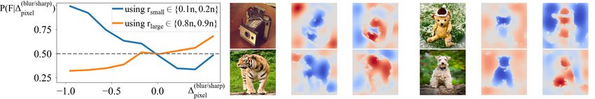
penalize small-scale concepts ||∆f (i, L)||2 of very few contextual pixels rsmall ∈ {0.1n, 0.2n}. The
second experiment was to punish large-scale concepts ||∆f (i, L)||2 of rlarge ∈ {0.8n, 0.9n}. Fig. 5
shows penalizing small-scale concepts ||∆f (i, L)||2 usually tended to sharpen the foreground and
blurred the background of images. It was because small-scale concepts usually referred to detailed
concepts at the pixel level for the classification of foreground objects, which made the DNN sharpen
pixel-wise patterns in the foreground (salient objects) and blur the background (irrelevant objects).
In contrast, punishing large-scale concepts ||∆f (i, L)||2 were prone to blurring the foreground and
sharpening the background. It was because large-scale concepts usually encoded global contextual
knowledge for the inference of objects (e.g. the background), which led to sharpening the background.
Although theoretically the background was sometimes also useful for classification, the using of
large-scale background knowledge for inference usually caused a higher cognitive burden than using
more direct features in the foreground. Therefore, a common aesthetic appreciation in photography
was to blur the background and sharpen the foreground.
Implementation details. We computed the loss function using the ResNet-18 model trained on the
ImageNet dataset, in order to revise images. As Fig. 5 shows, ∆(blur/sharp) pixel was a pixel in the heatmap
∆(blur/sharp) defined in Eq. (10), which measured whether this pixel was blurred or sharpened. Let
P (∆(blur/sharp)
 pixel |F ) denote the probability distribution of ∆(blur/sharp)
 pixel among all pixels in the foreground of
all images, where F indicated a set of all foreground pixels. Accordingly, P (∆(blur/sharp) pixel |B) represented
 (blur/sharp)
the probability distribution of ∆pixel among all pixels in the background of all images, where B de-
noted a set of all background pixels. Here, we used the object bounding box to separate the foreground
and the background of each image. In this way, given a certain value of ∆(blur/sharp) pixel , P (F |∆(blur/sharp)
 pixel ) de-
 (blur/sharp)
scribed the probability of the pixel with the sharpening/smoothing score ∆pixel locating in the fore-
ground, i.e. P (F |∆(blur/sharp)
 pixel ) = P (∆(blur/sharp)
 pixel |F )·P (F )/(P (∆(blur/sharp)
 pixel |F )·P (F )+P (∆(blur/sharp)
 pixel |B)·P (B)).
P (F ) and P (B) referred to the prior probability of foreground pixels or background pixels, respec-
tively. If P (F |∆(blur/sharp)
 pixel ) > 0.5, then the pixel with the sharpening/smoothing score ∆(blur/sharp) pixel was
more likely to locate in the foreground. Fig. 5 shows penalizing small-scale concepts ||∆f (i, L)||2 usu-
ally tended to sharpen the foreground and blur the background of images, i.e. P (F |∆(blur/sharp) pixel ) > 0.5
 (blur/sharp)
when ∆pixel < 0. In comparison, punishing large-scale concepts ||∆f (i, L)||2 often sharpened the
background and blurred the foreground.

 9

5 Conclusion
In this paper, we propose a hypothesis for the aesthetic appreciation that aesthetic images make a
neural network strengthen salient concepts and discard inessential concepts. In order to verify this
hypothesis, we use multi-variate interactions to represent salient concepts and inessential concepts
encoded in the DNN. Furthermore, we develop a new method to revise images, and find that the
revised images are more aesthetic than the original ones to some degree. Nevertheless, in spite of the
success in experiments and preliminary verifications, we still need further to verify the trustworthiness
of the hypothesis.

References
 [1] Jochen Baumeister, T Barthel, Kurt-Reiner Geiss, and M Weiss. Influence of phosphatidylserine
 on cognitive performance and cortical activity after induced stress. Nutritional neuroscience, 11
 (3):103–110, 2008.
 [2] Subhabrata Bhattacharya, Rahul Sukthankar, and Mubarak Shah. A framework for photo-
 quality assessment and enhancement based on visual aesthetics. In Proceedings of the 18th
 ACM international conference on Multimedia, pages 271–280, 2010.
 [3] George David Birkhoff. Aesthetic measure. Harvard University Press, 2013.
 [4] Yihang Bo, Jinhui Yu, and Kang Zhang. Computational aesthetics and applications. Visual
 Computing for Industry, Biomedicine, and Art, 1(1):1–19, 2018.
 [5] Jeffrey B Brookings, Glenn F Wilson, and Carolyne R Swain. Psychophysiological responses to
 changes in workload during simulated air traffic control. Biological psychology, 42(3):361–377,
 1996.
 [6] Steven Brown, Xiaoqing Gao, Loren Tisdelle, Simon B Eickhoff, and Mario Liotti. Naturalizing
 aesthetics: brain areas for aesthetic appraisal across sensory modalities. Neuroimage, 58(1):
 250–258, 2011.
 [7] Gyorgy Buzsaki. Rhythms of the Brain. Oxford University Press, 2006.
 [8] Camilo J Cela-Conde, Francisco J Ayala, Enric Munar, Fernando Maestú, Marcos Nadal,
 Miguel A Capó, David del Río, Juan J López-Ibor, Tomás Ortiz, Claudio Mirasso, et al. Sex-
 related similarities and differences in the neural correlates of beauty. Proceedings of the National
 Academy of Sciences, 106(10):3847–3852, 2009.
 [9] Kuang-Yu Chang, Kung-Hung Lu, and Chu-Song Chen. Aesthetic critiques generation for
 photos. In Proceedings of the IEEE International Conference on Computer Vision, pages
 3514–3523, 2017.
[10] Anjan Chatterjee. Neuroaesthetics: a coming of age story. Journal of cognitive neuroscience,
 23(1):53–62, 2011.
[11] Anjan Chatterjee and Oshin Vartanian. Neuroaesthetics. Trends in cognitive sciences, 18(7):
 370–375, 2014.
[12] Liang-Chieh Chen, Yukun Zhu, George Papandreou, Florian Schroff, and Hartwig Adam.
 Encoder-decoder with atrous separable convolution for semantic image segmentation. In
 Proceedings of the European conference on computer vision (ECCV), pages 801–818, 2018.
[13] Qiuyu Chen, Wei Zhang, Ning Zhou, Peng Lei, Yi Xu, Yu Zheng, and Jianping Fan. Adaptive
 fractional dilated convolution network for image aesthetics assessment. In Proceedings of
 the IEEE/CVF Conference on Computer Vision and Pattern Recognition, pages 14114–14123,
 2020.
[14] Yu-Sheng Chen, Yu-Ching Wang, Man-Hsin Kao, and Yung-Yu Chuang. Deep photo enhancer:
 Unpaired learning for image enhancement from photographs with gans. In Proceedings of the
 IEEE Conference on Computer Vision and Pattern Recognition, pages 6306–6314, 2018.

 10

[15] Piotr Dabkowski and Yarin Gal. Real time image saliency for black box classifiers. arXiv
 preprint arXiv:1705.07857, 2017.
[16] Ritendra Datta, Dhiraj Joshi, Jia Li, and James Z Wang. Studying aesthetics in photographic
 images using a computational approach. In European conference on computer vision, pages
 288–301. Springer, 2006.
[17] Yubin Deng, Chen Change Loy, and Xiaoou Tang. Aesthetic-driven image enhancement by
 adversarial learning. In Proceedings of the 26th ACM international conference on Multimedia,
 pages 870–878, 2018.
[18] Sagnik Dhar, Vicente Ordonez, and Tamara L Berg. High level describable attributes for
 predicting aesthetics and interestingness. In CVPR 2011, pages 1657–1664. IEEE, 2011.
[19] Robert E Dustman, Reed S Boswell, and Paul B Porter. Beta brain waves as an index of alertness.
 Science, 137(3529):533–534, 1962.
[20] Russell Epstein and Nancy Kanwisher. A cortical representation of the local visual environment.
 Nature, 392(6676):598–601, 1998.
[21] Seyed A Esmaeili, Bharat Singh, and Larry S Davis. Fast-at: Fast automatic thumbnail
 generation using deep neural networks. In Proceedings of the IEEE Conference on Computer
 Vision and Pattern Recognition, pages 4622–4630, 2017.
[22] Gustav Theodor Fechner. Vorschule der aesthetik, volume 1. Breitkopf & Härtel, 1876.
[23] Theodore Gracyk. Hume’s aesthetics. 2003.
[24] Mark W Greenlee and U Tse Peter. Functional neuroanatomy of the human visual system:
 A review of functional mri studies. Pediatric ophthalmology, neuro-ophthalmology, genetics,
 pages 119–138, 2008.
[25] Kai Hammermeister. The German aesthetic tradition. Cambridge University Press, 2002.
[26] Vlad Hosu, Bastian Goldlucke, and Dietmar Saupe. Effective aesthetics prediction with multi-
 level spatially pooled features. In Proceedings of the IEEE/CVF Conference on Computer
 Vision and Pattern Recognition, pages 9375–9383, 2019.
[27] Thomas Jacobsen and Susan Beudt. Domain generality and domain specificity in aesthetic
 appreciation. New Ideas in Psychology, 47:97–102, 2017.
[28] Thomas Jacobsen, Ricarda I Schubotz, Lea Höfel, and D Yves v Cramon. Brain correlates of
 aesthetic judgment of beauty. Neuroimage, 29(1):276–285, 2006.
[29] Bin Jin, Maria V Ortiz Segovia, and Sabine Süsstrunk. Image aesthetic predictors based on
 weighted cnns. In 2016 IEEE International Conference on Image Processing (ICIP), pages
 2291–2295. Ieee, 2016.
[30] Xin Jin, Le Wu, Geng Zhao, Xiaodong Li, Xiaokun Zhang, Shiming Ge, Dongqing Zou, Bin
 Zhou, and Xinghui Zhou. Aesthetic attributes assessment of images. In Proceedings of the 27th
 ACM International Conference on Multimedia, pages 311–319, 2019.
[31] Victor S Johnston. Mate choice decisions: the role of facial beauty. Trends in cognitive sciences,
 10(1):9–13, 2006.
[32] Shaoqing Ren Kaiming He, Xiangyu Zhang and Jian Sun. Deep residual learning for image
 recognition. In CVPR, 2016.
[33] Yueying Kao, Ran He, and Kaiqi Huang. Deep aesthetic quality assessment with semantic
 information. IEEE Transactions on Image Processing, 26(3):1482–1495, 2017.
[34] Yan Ke, Xiaoou Tang, and Feng Jing. The design of high-level features for photo quality
 assessment. In 2006 IEEE Computer Society Conference on Computer Vision and Pattern
 Recognition (CVPR’06), volume 1, pages 419–426. IEEE, 2006.

 11

[35] Han-Ul Kim, Young Jun Koh, and Chang-Su Kim. Pienet: Personalized image enhancement
 network. In European Conference on Computer Vision, pages 374–390. Springer, 2020.
[36] Jin-Hwan Kim, Won-Dong Jang, Jae-Young Sim, and Chang-Su Kim. Optimized contrast
 enhancement for real-time image and video dehazing. Journal of Visual Communication and
 Image Representation, 24(3):410–425, 2013.
[37] Louise P Kirsch, Cosimo Urgesi, and Emily S Cross. Shaping and reshaping the aesthetic
 brain: Emerging perspectives on the neurobiology of embodied aesthetics. Neuroscience &
 Biobehavioral Reviews, 62:56–68, 2016.
[38] Shu Kong, Xiaohui Shen, Zhe Lin, Radomir Mech, and Charless Fowlkes. Photo aesthetics
 ranking network with attributes and content adaptation. In European Conference on Computer
 Vision, pages 662–679. Springer, 2016.
[39] Alex Krizhevsky, Ilya Sutskever, and Geoffrey E Hinton. Imagenet classification with deep
 convolutional neural networks. Advances in neural information processing systems, 25:1097–
 1105, 2012.
[40] Helmut Leder, Benno Belke, Andries Oeberst, and Dorothee Augustin. A model of aesthetic
 appreciation and aesthetic judgments. British journal of psychology, 95(4):489–508, 2004.
[41] Joon-Young Lee, Kalyan Sunkavalli, Zhe Lin, Xiaohui Shen, and In So Kweon. Automatic
 content-aware color and tone stylization. In Proceedings of the IEEE conference on computer
 vision and pattern recognition, pages 2470–2478, 2016.
[42] Leida Li, Hancheng Zhu, Sicheng Zhao, Guiguang Ding, and Weisi Lin. Personality-assisted
 multi-task learning for generic and personalized image aesthetics assessment. IEEE Transactions
 on Image Processing, 29:3898–3910, 2020.
[43] Rui Li and Junsong Zhang. Review of computational neuroaesthetics: bridging the gap between
 neuroaesthetics and computer science. Brain Informatics, 7(1):1–17, 2020.
[44] Dong Liu, Rohit Puri, Nagendra Kamath, and Subhabrata Bhattacharya. Composition-aware im-
 age aesthetics assessment. In Proceedings of the IEEE/CVF Winter Conference on Applications
 of Computer Vision, pages 3569–3578, 2020.
[45] Kin Gwn Lore, Adedotun Akintayo, and Soumik Sarkar. Llnet: A deep autoencoder approach
 to natural low-light image enhancement. Pattern Recognition, 61:650–662, 2017.
[46] Xin Lu, Zhe Lin, Hailin Jin, Jianchao Yang, and James Z Wang. Rapid: Rating pictorial
 aesthetics using deep learning. In Proceedings of the 22nd ACM international conference on
 Multimedia, pages 457–466, 2014.
[47] Xin Lu, Zhe Lin, Hailin Jin, Jianchao Yang, and James Z Wang. Rating image aesthetics using
 deep learning. IEEE Transactions on Multimedia, 17(11):2021–2034, 2015.
[48] Qiuling Luo, Mengxia Yu, You Li, and Lei Mo. The neural correlates of integrated aesthetics
 between moral and facial beauty. Scientific reports, 9(1):1–10, 2019.
[49] Wei Luo, Xiaogang Wang, and Xiaoou Tang. Content-based photo quality assessment. In 2011
 International Conference on Computer Vision, pages 2206–2213. IEEE, 2011.
[50] Shuang Ma, Jing Liu, and Chang Wen Chen. A-lamp: Adaptive layout-aware multi-patch
 deep convolutional neural network for photo aesthetic assessment. In Proceedings of the IEEE
 Conference on Computer Vision and Pattern Recognition, pages 4535–4544, 2017.
[51] Long Mai, Hailin Jin, and Feng Liu. Composition-preserving deep photo aesthetics assessment.
 In Proceedings of the IEEE conference on computer vision and pattern recognition, pages
 497–506, 2016.
[52] Luca Marchesotti, Florent Perronnin, Diane Larlus, and Gabriela Csurka. Assessing the aesthetic
 quality of photographs using generic image descriptors. In 2011 international conference on
 computer vision, pages 1784–1791. IEEE, 2011.

 12

[53] Luca Marchesotti, Florent Perronnin, and France Meylan. Learning beautiful (and ugly)
 attributes. In BMVC, volume 7, pages 1–11, 2013.
[54] Naila Murray, Luca Marchesotti, and Florent Perronnin. Ava: A large-scale database for
 aesthetic visual analysis. In 2012 IEEE Conference on Computer Vision and Pattern Recognition,
 pages 2408–2415. IEEE, 2012.
[55] L Neumann, M Sbert, B Gooch, W Purgathofer, et al. Defining computational aesthetics.
 Computational aesthetics in graphics, visualization and imaging, pages 13–18, 2005.
[56] Masashi Nishiyama, Takahiro Okabe, Imari Sato, and Yoichi Sato. Aesthetic quality classifica-
 tion of photographs based on color harmony. In CVPR 2011, pages 33–40. IEEE, 2011.
[57] Marcus T Pearce, Dahlia W Zaidel, Oshin Vartanian, Martin Skov, Helmut Leder, Anjan
 Chatterjee, and Marcos Nadal. Neuroaesthetics: The cognitive neuroscience of aesthetic
 experience. Perspectives on psychological science, 11(2):265–279, 2016.
[58] Jie Ren, Zhanpeng Zhou, Qirui Chen, and Quanshi Zhang. Learning baseline values for shapley
 values, 2021.
[59] L. Shapley. A value for n-person games. 1953.
[60] James Shelley. The concept of the aesthetic. 2017.
[61] Kekai Sheng, Weiming Dong, Menglei Chai, Guohui Wang, Peng Zhou, Feiyue Huang, Bao-
 Gang Hu, Rongrong Ji, and Chongyang Ma. Revisiting image aesthetic assessment via self-
 supervised feature learning. In Proceedings of the AAAI Conference on Artificial Intelligence,
 volume 34, pages 5709–5716, 2020.
[62] Karen Simonyan and Andrew Zisserman. Very deep convolutional networks for large-scale
 image recognition. In ICLR, 2015.
[63] Hanghang Tong, Mingjing Li, Hong-Jiang Zhang, Jingrui He, and Changshui Zhang. Classifi-
 cation of digital photos taken by photographers or home users. In Pacific-Rim Conference on
 Multimedia, pages 198–205. Springer, 2004.
[64] Yi Tu, Li Niu, Weijie Zhao, Dawei Cheng, and Liqing Zhang. Image cropping with composition
 and saliency aware aesthetic score map. In Proceedings of the AAAI Conference on Artificial
 Intelligence, volume 34, pages 12104–12111, 2020.
[65] Edward A Vessel and Nava Rubin. Beauty and the beholder: Highly individual taste for abstract,
 but not real-world images. Journal of vision, 10(2):18–18, 2010.
[66] Wenshan Wang, Su Yang, Weishan Zhang, and Jiulong Zhang. Neural aesthetic image reviewer.
 IET Computer Vision, 13(8):749–758, 2019.
[67] Zhangyang Wang, Ding Liu, Shiyu Chang, Florin Dolcos, Diane Beck, and Thomas Huang.
 Image aesthetics assessment using deep chatterjee’s machine. In 2017 International Joint
 Conference on Neural Networks (IJCNN), pages 941–948. IEEE, 2017.
[68] Robert J Weber. Probabilistic values for games, the shapley value. essays in honor of lloyd s.
 shapley (ae roth, ed.), 1988.
[69] Zijun Wei, Jianming Zhang, Xiaohui Shen, Zhe Lin, Radomír Mech, Minh Hoai, and Dimitris
 Samaras. Good view hunting: Learning photo composition from dense view pairs. In Proceed-
 ings of the IEEE Conference on Computer Vision and Pattern Recognition, pages 5437–5446,
 2018.
[70] Ou Wu, Weiming Hu, and Jun Gao. Learning to predict the perceived visual quality of photos.
 In 2011 International Conference on Computer Vision, pages 225–232. IEEE, 2011.
[71] Saining Xie and Zhuowen Tu. Holistically-nested edge detection. In Proceedings of the IEEE
 international conference on computer vision, pages 1395–1403, 2015.

 13

[72] Jianzhou Yan, Stephen Lin, Sing Bing Kang, and Xiaoou Tang. Change-based image cropping
 with exclusion and compositional features. International Journal of Computer Vision, 114(1):
 74–87, 2015.
[73] Semir Zeki. A vision of the brain. Blackwell scientific publications, 1993.
[74] Semir Zeki. Art and the brain. Journal of Consciousness Studies, 6(6-7):76–96, 1999.
[75] Hui Zeng, Lida Li, Zisheng Cao, and Lei Zhang. Reliable and efficient image cropping: A grid
 anchor based approach. In Proceedings of the IEEE/CVF Conference on Computer Vision and
 Pattern Recognition, pages 5949–5957, 2019.
[76] Quanshi Zhang, Xin Wang, Ruiming Cao, Ying Nian Wu, Feng Shi, and Song-Chun Zhu.
 Extracting an explanatory graph to interpret a cnn. IEEE transactions on pattern analysis and
 machine intelligence, 2020.
[77] Ye Zhou, Xin Lu, Junping Zhang, and James Z Wang. Joint image and text representation for
 aesthetics analysis. In Proceedings of the 24th ACM international conference on Multimedia,
 pages 262–266, 2016.

 14

A Proof of the closed-form solution to the multi-variate interaction in Eq.
 (2)

The multi-variate interaction I(S) defined in [58] measures the marginal utility from the collaboration
of input pixels in the pattern S, in comparison with the utility when these pixels work individually.
Specifically, let f (S) − f (∅) denote the overall utility received
 P P in S. Then, we remove
 from all pixels
utilities of individual pixels without collaborations, i.e. i∈S v({i}) = i∈S (f ({i}) − f (∅)), and
further remove the marginal utilities owing to collaborations of all smaller compositional patterns
L within S, i.e. L ( S||L| ≥ 2 . In this way, the multi-variate interaction I(S) defined in [58] is
given as follows.

 X X
 I(S) = f (S) − f (∅) − I(L) − v({i}). (11)
 | {z }
 L$S,|L|≥2 i∈S
 the utility of all pixels in S

The closed-form solution for Eq. (11) is proven as follows.

 X
 I(S) = (−1)|S|−|L| f (L). (12)
 L⊆S

• Proof : Here, let s = |S|, l = |L|, and s0 = |S 0 | for simplicity. If s = 2, then

 X X
 I(S) = f (S) − f (∅) − I(L) − v({i})
 L$S,l≥2 i∈S
 X
 = f (S) − f (∅) − v({i})
 i∈S
 X
 = f (S) − f (∅) − [f ({i}) − f (∅)]
 i∈S
 X
 = f (S) − f ({i}) + f (∅)
 i∈S
 X
 = (−1)s−l f (L)
 L⊆S

 15

0
Let us assume that if 2 ≤ s0 < s, I(S 0 ) = L⊆S 0 (−1)s −l f (L). Then, we use the mathematical
 P

induction to prove I(S) = L⊆S (−1)s−l f (L), where S 0 $ S.
 P

 X X
 I(S = S 0 ∪ {i}) =f (S 0 ∪ {i}) − f (∅) − I(L) − v({j}) % Let S = S 0 ∪ {i}
 0 j∈S 0 ∪{i}
 L$S ∪{i},
 l≥2
 X X X
 =f (S 0 ∪ {i}) − f (∅) − (−1)l−k f (K) − v({j})
 L$S 0 ∪{i}, K⊆L j∈S 0 ∪{i}
 l≥2
 X X
 =f (S 0 ∪ {i}) − f (∅) − (−1)t f (K)
 K$S 0 0
 T ⊆S ∪{i}\K,
 t+s0 ≥2
 X
 − v({j}) % Let T = L \ K
 j∈S 0 ∪{i}
 0
 s0
 X X sX −1
 =f (S 0 ∪ {i}) − f (∅) − Cst0 +1 (−1)t f (∅) + Cst0 (−1)t f ({j})
 t=2 j∈S 0 ∪{i} t=1
 0
 X sX −k  X
 + Cst0 +1−k (−1)t f (K) − v({j})
 K$S 0 ∪{i}, t=0 j∈S 0 ∪{i}
 k≥2
 0 X 0
 =f (S 0 ∪ {i}) − f (∅) − (s0 − (−1)s +1
 )v(∅) + (1 + (−1)s )f ({j})
 j∈S∪{i}
 s0 +1−k
 X X
 + (−1) f (K) − [f ({i}) − f (∅)]
 K$S 0 ∪{i}, j∈S 0 ∪{i}
 k≥2
 X 0 0 X 0
 =f (S 0 ∪ {i}) + (−1)s f ({j}) + (−1)s +1
 f (∅) + (−1)s +1−k
 f (K)
 j∈S 0 ∪{i} K$S 0 ∪{i},
 k≥2
 X 0 X
 = (−1)s +1−k
 f (K) = (−1)s−k f (K)
 K⊆S 0 ∪{i} K⊆S

 In this way, Equation (12) is proven as the closed-form solution to the definition of the multi-variate
interaction I(S) in Equation (11).

B Proof of the decomposition of classification utilities in Eq. (3)
Mathematically, we have proven that the classification utilities of all pixels, f (N ) − f (∅), can be
decomposed as the sum of utilities of different interaction patterns. In other words, the discrimination
power can be decomposed as the sum of classification utilities of massive elementary concepts.
 X X
 f (N ) − f (∅) − v({i}) = S⊆N, I(S) (13)
 i∈N
 |S|≥2

• Proof :
 X X X X X
 I(S) + f (∅) + v({i}) = (−1)|S|−|L| f (L) + f (∅) + [f ({i}) − f (∅)]
 S⊆N, i∈N S⊆N, L⊆S i∈N
 |S|≥2 |S|≥2
 X X
 = (−1)|S|−|L| f (L)
 S⊆N L⊆S
 X X
 = (−1)|K| f (L) % Let K = S \ L
 L⊆N K⊆N \L
  
 n−|L|
 |K|
 X X
 =  Cn−|L| (−1)|K|  f (L) = f (N )
 L⊆N |K|=0

 16

C Detailed introduction of Shapley values
The Shapley value [59] defined in game theory is widely considered as an unbiased estimation of the
numerical utility w.r.t. each input pixel. Given a trained DNN f and an image x ∈ Rn with n pixels
N = {1, 2, · · · , n}, some pixels may cooperate to form a context L ⊆ N to influence the output
y = f (x) ∈ R. To this end, the Shapley value is proposed to fairly divide and assign the overall
effects on the network output to each pixel. In this way, the Shapley value, φ(i|N ), represents the
utility of the pixel i to the network output, as follows.
 X (n − |L| − 1)!|L|! h i
 φ(i|N ) = ∆f (i, L) , (14)
 L⊆N \{i} n!
 def
where ∆f (i, L) = f (L ∪ {i}) − f (L) measures the marginal utility of the pixel i to the network
output, given a set of contextual pixels L.
Weber [68] has proven that the Shapley value is a unique method to fairly allocate the overall utility
to each pixel that satisfies following properties.
(1) Linearity property: If two independent DNNs can be merged into one DNN, then the Shapley
value of the new DNN also can be merged, i.e. ∀i ∈ N , φu (i|N ) = φv (i|N ) + φw (i|N ); ∀c ∈ R,
φc·u (i|N ) = c · φu (i|N ).
(2) Nullity property: The dummy pixel i is defined as a pixel satisfying ∀S ⊆ N \ {i}, v(S ∪
{i}) = v(S) + v({i}), which indicates that the pixel i has no interactions with other pixels in N ,
φ(i|N ) = v({i}) − v(∅).
(3) Symmetry property: If ∀S ⊆ N \ {i, j}, v(S ∪ {i}) = v(S ∪ {j}), then φ(i|N ) = φ(j|N ).
 P
(4) Efficiency property: Overall utility can be assigned to all pixels, i∈N φ(i|N ) = v(N ) − v(∅).

D Proof of Eq. (5)
We have proven that the term ∆f (i, L) in the Shapley value can be re-written as the sum of some
interaction patterns.
 X
 ∆f (i, L) = v({i}) + 0 0
 I(S 0 = L0 ∪ {i}). (15)
 L ⊆L,L 6=∅
• Proof :
 X
 right = v({i}) + 0 0 I(S 0 = L0 ∪ {i})
 L ⊆L,L 6=∅
 X h X 0
 = v({i}) + (−1)|L |+1−|K|
 f (K)
 0 0
 L ⊆L, K⊆L
 0
 L 6=∅
 0
 X i
 + (−1)|L |−|K|
 f (K ∪ {i}) % Based on Eq. (12)
 0
 K⊆L
 X X 0
 = v({i}) + (−1)|L |−|K|
 [f (K ∪ {i}) − f (K)]
 0 0 0
 L ⊆L,L 6=∅ K⊆L
 X X 0
 = (−1)|L |−|K|
 ∆f (i, K)
 0 0
 L ⊆L K⊆L
 X X
 = (−1)|P | ∆f (i, K) % Let P = L0 \ K
 K⊆L P ⊆L\K
  
 |L|−|K|
 X X p p
 =  (−1) C|L|−|K|  ∆f (i, K) % Let p = |P |
 K⊆L p=0
  
 |L|−|K|
 X X X p p
 = 0 · ∆f (i, K) +  (−1) C|L|−|K|  ∆f (i, K)
 K$L K=L p=0

 = ∆f (i, L) = left

 17