A Method for Human Facial Image Annotation on Low Power Consumption Autonomous Devices - MDPI
←
→
Page content transcription
If your browser does not render page correctly, please read the page content below
sensors
Article
A Method for Human Facial Image Annotation on Low
Power Consumption Autonomous Devices
Tomasz Hachaj
 Institute of Computer Science, Pedagogical University of Krakow, 2 Podchorazych Ave, 30-084 Krakow, Poland;
 tomekhachaj@o2.pl

 Received: 9 March 2020; Accepted: 8 April 2020; Published: 10 April 2020

 Abstract: This paper proposes a classifier designed for human facial feature annotation, which is capable
 of running on relatively cheap, low power consumption autonomous microcomputer systems. An
 autonomous system is one that depends only on locally available hardware and software—for example,
 it does not use remote services available through the Internet. The proposed solution, which consists of
 a Histogram of Oriented Gradients (HOG) face detector and a set of neural networks, has comparable
 average accuracy and average true positive and true negative ratio to state-of-the-art deep neural network
 (DNN) architectures. However, contrary to DNNs, it is possible to easily implement the proposed method
 in a microcomputer with very limited RAM memory and without the use of additional coprocessors.
 The proposed method was trained and evaluated on a large 200,000 image face data set and compared
 with results obtained by other researchers. Further evaluation proves that it is possible to perform facial
 image attribute classification using the proposed algorithm on incoming video data captured by an RGB
 camera sensor of the microcomputer. The obtained results can be easily reproduced, as both the data set
 and source code can be downloaded. Developing and evaluating the proposed facial image annotation
 algorithm and its implementation, which is easily portable between various hardware and operating
 systems (virtually the same code works both on high-end PCs and microcomputers using the Windows
 and Linux platforms) and which is dedicated for low power consumption devices without coprocessors,
 is the main and novel contribution of this research.

 Keywords: facial image annotation; RGB camera sensor; neural network; deep neural network;
 eigenfaces; nearest neighbour classifier; low power consumption computer

1. Introduction
      Facial image analysis and classification is among the most important and up-to-date tasks in computer
vision, signal processing, and pattern recognition methods. By looking at a human face, we can identify
not only the most general features, such as gender, race, and age, but also facial expression (emotions)
and recollect their identity (i.e., whether that person was met before). The ability of facial image analysis
is basic and is among the most important human-to-human interaction processes. Lately, due to the
development of novel machine learning algorithms (especially deep learning) and access to large data sets
of facial images, it has become possible to automate some facial recognition approaches by using computer
methods. In the following subsections, various applications of those algorithms and the contributions of
this paper will be discussed.

Sensors 2020, 20, 2140; doi:10.3390/s20072140                                     www.mdpi.com/journal/sensors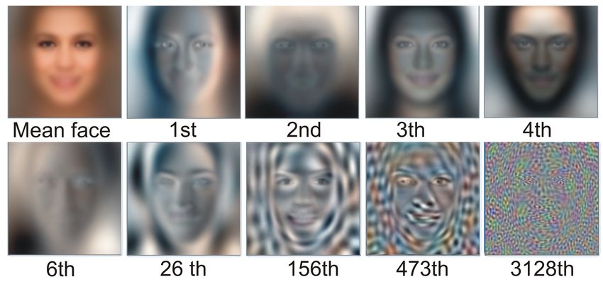
Sensors 2020, 20, 2140                                                                                 2 of 16

1.1. Face Recognition
     Before facial images can be processed, there are several pre-processing steps that have to be done.
Traditionally, one needs to cascade two blocks: face localization and facial descriptor construction [1]. In
some studies, these steps are replaced by applying a single deep neural network (DNN) architecture [2,3].
Facial recognition systems were applied in many computer systems, from real-time face tracking and
recognition systems [4] and identification of people in personal smartphone galleries [5] to large-scale
classification and security systems [6]. Chang et al. [7] proposed a facial recognition algorithm based
on a support vector machine (SVM) combined with Visual Geometry Group (VGG) network model
for extracting facial features, which not only accurately extracts face features, but also reduces feature
dimensions and avoids irrelevant features in the calculation. However, some researchers continue to use
the well-known eigenfaces approaches, using the Euclidean distance measure [8]. Among the up-to-date
problems in face recognition is the age-invariant face recognition task [9]. At the same time, the tactics
used to mislead these systems have become more complex and counter-measure approaches are necessary.
For example, Lucena et al. [10] proposed an approach based on transfer learning with a pre-trained
convolutional neural network (CNN) model, which uses only static features to recognize photo, video,
or mask attacks.

1.2. Face Attribute Prediction and Annotation
      A facial image can be described (annotated) with many important features, such as gender, race,
shape of the chin, hair colour, and so on. Zhong et al. [1], Aly et al. [11], and Fan et al. [12] achieved
these goals using descriptors constructed from different levels of the CNNs for different attributes to best
facilitate face attribute prediction. Yilmaztürk et al. [13] studied automatic and online face annotation for
personal videos/episodes of TV series considering Nearest Neighbour, Linear discriminant analysis (LDA),
and SVM classification with Local Binary Patterns, Discrete Cosine Transform, and Histogram of Oriented
Gradients feature extraction methods, considering their recognition accuracies and execution times.
      Facial image annotation can be also applied in content-based image retrieval (CBIR). These types of
systems find images within a database that are similar to query. Conilione et al. [14], Nguyen et al. [15],
and Wang et al. [16] attempted to discover semantic labels for facial features for use in such systems.
      Chang et al. [17] described the use of an unsupervised label refinement (ULR) method for the task of
fixing weakly labelled facial image data collected from the Internet with mislabelled images. To improve
the correction accuracy of ULR, particle swarm optimization (PSO) and binary particle swarm optimization
(BPSO) were used to solve the binary constraint optimization task in that study. Firmino et al. [18] used
automatic and semi-automatic annotation techniques for people in photos using the shared event concept,
which consists of many photos captured by different devices of people who attended the same event.
Among the most popular and efficient approaches for facial image annotation are various convolutional
neural networks (CNNs) [1,19–22].
      Additional large surveys of describable visual face attributes which can be applied in face recognition
and annotation can be found in [23,24].

1.3. Other Computer Methods That Use Facial Images
     Among the other methods based on facial images, we mention face completion methods, the goal
of which is to reconstruct facial image from incomplete or obscure data. Zhang et al. [25] reported
using a symmetry-aware face completion method based on facial structural features found using a deep
generative model. The model is trained with a combination of a reconstruction loss, a structure loss, two
adversarial losses, and a symmetry loss, which ensures pixel faithfulness, local–global content integrity,
and symmetric consistency. Low-resolution facial images might be also used as input for attribute-guided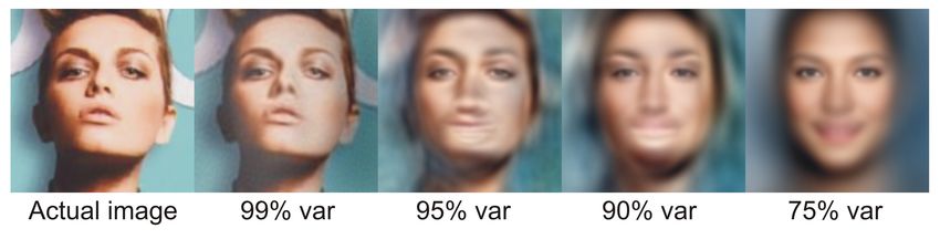
Sensors 2020, 20, 2140                                                                               3 of 16

face generation systems [26]. The massive potential of face recognition methods poses a serious privacy
threat to individuals who do not want to be profiled. Chhabra et al. [27] and Flouty et al. [28] presented
novel algorithms for anonymizing selective attributes which an individual does not want to share, without
affecting the visual quality of facial images.

1.4. Contributions of This Research
     Due to ongoing miniaturization of the computer hardware, there are many affordable low power
consumption microcomputer platforms which can be used for general purpose computing. Low power
consumption means hardware-powered; for example, by USB standard (5 V, 3 A). Such platforms typically
have limited computational power (CPU) and memory (both RAM and disc); however, they can be easily
deployed in many types of mobile and/or autonomous systems. An autonomous system depends only on
locally available hardware and software; for example, it cannot use remote services available through the
Internet. Despite the limitations of such hardware, novel multi-platform machine learning frameworks
have made it possible to create implementations of face analysis algorithms that can be deployed across
multiple types of hardware architectures and operation systems.
     The aim of this paper is to design, train, evaluate, and implement a facial image processing algorithm
which can perform face annotation based on images from a single RGB camera which has accuracy at the
level of state-of-the art pattern recognition methods and which can be run on a low power consumption
microcomputer. This goal is usually solved by training a classifier on another computer and then deploying
the trained model onto a microcomputer which is supported by an additional co-processor. However, the
inclusion of a co-processor increases the price of the hardware: depending on the platform we choose,
the coprocessor may cost three times more than the microcomputer itself. This is a large increment of
cost, especially if the system we want to create contains many separate microcomputers; for example, if
each is a component of an individual patrolling robot. Due to this, the second assumption of this paper
is that the proposed annotation method should be successfully deployed and run on a microcomputer
without the aid of additional external computing modules. Of course, the classifier training procedure
has to done on different hardware in order to be finished in reasonable time. In this paper, I will detail
how this method has been developed, beginning from training on a large (over 200,000 images) data set,
comparison with the state-of-the-art methods, and running it on a popular low power consumption device.
I used popular hardware and machine learning platform solutions and all source code was published,
such that the results I obtained can be reproduced. Developing and evaluating the proposed facial image
annotation algorithm and its implementation, which is easily portable between various hardware and
operating systems (virtually the same code works both on high-end PCs and microcomputers using the
Windows and Linux platforms) and which is dedicated for low power consumption devices without
coprocessors, is the main and novel contribution of this research.

2. Material and Methods
     In this section, the data set on which the training and validation of the proposed face annotation
algorithm has been done will be presented. Furthermore, I will discuss the proposed method and details
of the state-of-the-art methods which the proposed method was compared to.

2.1. The Data Set
     The data set that was used in this research is Large-scale CelebFaces Attributes (CelebA) [19]. It can
be downloaded from the Internet (http://mmlab.ie.cuhk.edu.hk/projects/CelebA.html). It contains over
200,000 pictures, mostly of actors, celebrities, sports players, and so on. Each image is described with
40 attribute annotations. As can be seen in Table 1, all attributes are binary, indicating the true/false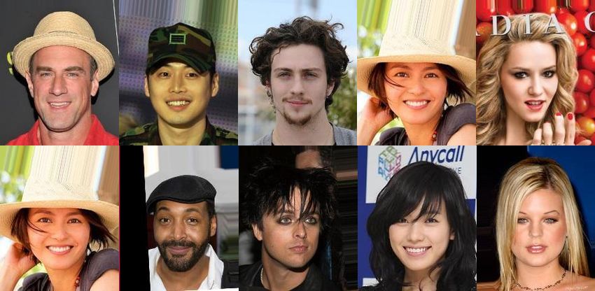
Sensors 2020, 20, 2140                                                                                           4 of 16

condition of some annotations (classes); for example, gender, having a double chin, having a mustache,
and so on. Although the distribution of images in the whole data set is random (there is no ordering of
images that, for example, separates males from females), there is large imbalance [19] in the annotation
classes: for example, only 4.15% of images have mustaches. This is an additional factor that makes classifier
training more challenging. As data set pictures were taken “in the wild“, there is a large variety in terms
of backgrounds and overall picture quality (contrast, saturation, and so on). In this research, I chose the
“Align and cropped images” version of this data set, which was initially pre-processed by a procedure
similar to the one described in Section 2.3. Figure 1 presents several samples from the data set.

      Table 1. The distribution of binary annotations in the data set. For example, 4.15% of images contain people
      with mustaches.

                                          Feature Name           True      False
                                      X5_o_Clock_Shadow         11.11%    88.89%
                                       Arched_Eyebrows           26.7%     73.3%
                                           Attractive           51.25%    48.75%
                                       Bags_Under_Eyes          20.46%    79.54%
                                              Bald               2.24%    97.76%
                                             Bangs              15.16%    84.84%
                                            Big_Lips            24.08%    75.92%
                                           Big_Nose             23.45%    76.55%
                                          Black_Hair            23.93%    76.07%
                                          Blond_Hair             14.8%     85.2%
                                             Blurry              5.09%    94.91%
                                          Brown_Hair            20.52%    79.48%
                                       Bushy_Eyebrows           14.22%    85.78%
                                            Chubby               5.76%    94.24%
                                         Double_Chin             4.67%    95.33%
                                           Eyeglasses            6.51%    93.49%
                                             Goatee              6.28%    93.72%
                                           Gray_Hair             4.19%    95.81%
                                        Heavy_Makeup            38.69%    61.31%
                                       High_Cheekbones           45.5%     54.5%
                                              Male              41.68%    58.32%
                                      Mouth_Slightly_Open       48.34%    51.66%
                                           Mustache              4.15%    95.85%
                                         Narrow_Eyes            11.51%    88.49%
                                           No_Beard             83.49%    16.51%
                                           Oval_Face            28.41%    71.59%
                                           Pale_Skin             4.29%    95.71%
                                         Pointy_Nose            27.74%    72.26%
                                       Receding_Hairline         7.98%    92.02%
                                         Rosy_Cheeks             6.57%    93.43%
                                           Sideburns             5.65%    94.35%
                                            Smiling             48.21%    51.79%
                                         Straight_Hair          20.84%    79.16%
                                          Wavy_Hair             31.96%    68.04%
                                       Wearing_Earrings         18.89%    81.11%
                                         Wearing_Hat             4.85%    95.15%
                                       Wearing_Lipstick         47.24%    52.76%
                                       Wearing_Necklace          12.3%     87.7%
                                       Wearing_Necktie           7.27%    92.73%
                                             Young              77.36%    22.64%
Sensors 2020, 20, 2140 5 of 16
Figure 1. Several random pictures from the CelebA dataset, which was used in this research. The images
were aligned and cropped such that eyes of each person are approximately in the same position. The faces
were also rescaled, such that they have similar size.
This data set has been intensively used by many researchers to evaluate face annotation methods.
Table 2 presents the accuracy (expressed in percentage) of some selected methods. As can be seen, the
highest reported accuracy was 91.00% for the method of [22], which uses the MobileNetV2 DNN network.
Therefore, I discuss this approach in next section and performed extensive comparisons of the results
obtained by MobileNetV2 with those of the method proposed in this paper.
Table 2. The accuracy (expressed in percentage) of various state-of-the-art methods in the task of image
annotation on the CelebA data set.
Method Accuracy
LNet [19] 85.00
LNet+ANet [1] 87.00
CNN+SVM [20] 89.80
ft +Color+LBP+SIFT [21] 90.22
MobileNetV2 [22] 91.00
2.2. Mobilenetv2
Among the papers reviewed in the first section of this paper, the highest annotation accuracy on
the CelebA data set has been reported by Luca et al. [22], where the authors used the DNN architecture
MobileNetV2 [19], but without the top classification layers. The architecture of MobileNetV2 contains
an initial convolutional layer with 32 filters, followed by 19 residual bottleneck layers. The kernel size
is always 3 × 3 and dropout and batch normalization were used during training. The top layers were
replaced by a dense (fully connected) network layer of size 1536 with the Rectified Linear Unit (ReLU)
activation function:
relu( x ) = max ( x, 0) (1)Sensors 2020, 20, 2140 6 of 16
That layer is followed by a batch normalization layer [29], followed by a dropout layer [30] and,
finally, a dense layer of size 37 with sigmoid activation function:
1
σ( x) = (2)
1 + e− x
The size of the input layer was a choice of the authors. The number of neurons in the output layer
is equal to number of attributes that are classified by the network. The authors decided to skip three
attributes of CelebA; namely Attractive, Pale_Skin, and Blurry. The output from the network is a single
37-dimensional vector, in which each value represents the classification of separate annotations of the
input image. Facial images were scaled to a uniform resolution of 224 × 244 pixels in RGB colour space.
The network was trained on about 180,000 images from the CelebA data set. The rest of the data set was
used for validation purposes. I adapted the same division of the data set for all methods evaluated in
this research.
To potentially increase generalization ability, the data set was augmented by various transforms
before training (i.e., rotation, width and height shifts, shearing, zooming, and horizontal flip), while
the parameters of the transforms were randomly changed between samples. The training algorithm
was AdaDelta [31], a gradient descent method that dynamically adapts over time using only first-order
information. In AdaDelta, the update of parameter y in the tth iteration is 4yt :
y t +1 = y t + 4 y t (3)
(
4 y0 = 0
(4)
4yt = − RMS [4y]t−1
RMS[ g]
gt
t
where RMS[4y]t−1 is the root mean square of the previous updates of 4y up to time t − 1 and RMS[ g]t
is root mean square of the previous square gradients g up to time t.
A loss function (optimization score function) was derived from the cosine similarity function defined
as the dot (scalar) product between the normalized reference r and predicted p vectors:
r·p
loss(r, p) = − (5)
|r | | p |
where · is the dot product and |r | is the norm of a vector r.
The metric to be evaluated by the model during training and testing was binary accuracy, which is
defined as an averaged value of how many times the rounded values of binary predictions are equal to the
actual value.
There were no obstacles to extending the output layer to 40 neurons and to train the network from
scratch to classify all 40 attributes. I performed these extensions and training. The results are described in
the Results and Discussion sections.
2.3. Histogram of Oriented Gradients Feature Descriptor and Neural Network
As was described in the previous section, an appropriately designed DNN can perform both face
feature detection and annotation. It is, however, possible to perform those tasks using other approaches.
Among the most popular methods for objects detection is the Histogram of Oriented Gradients (HOG)
method [32]. This method is implemented by dividing the image window into small spatial regions (“cells”)
and accumulating a local 1-D histogram of gradient directions (or edge orientations) over the pixels of each
cell. In this research, I used HOG features combined with image pyramid and sliding window to handling
various scales and object position and the SVM algorithm for classification. The face position estimator wasSensors 2020, 20, 2140 7 of 16
created using dlib’s implementation of the work of Kazemi et al. [33] and it was trained on the iBUG 300-W
face landmark data set [34]; the estimator is available online (https://github.com/davisking/dlib-models).
In this particular implementation, a set of 68 landmarks on the face is detected, which can be used to align
and rescale the face using basic image transforms such as translation, rotation, and scaling. All images in
both the training and validation data sets were aligned and scaled to the same size (128 × 128 pixels) in
RGB colour space. The images were used as an input to the classification algorithm, which was trained
to perform image annotations. The process of classification was divided into 40 separate neural network
classifiers. Each network was trained separately on each attribute using all images from the training data
set, which were aligned by the previously mentioned procedure. Each of the 40 neural networks is a
binary classifier, and they all shared the same architecture: a flattened input layer of size 128 × 128 × 3
that transforms the input RGB image into a vector, followed by a dense layer with 128 neurons which use
the ReLU activation function and, finally, a dense layer with two neurons using softmax activation.
e xi
so f tmax ( xi ) = x (6)
∑j e j
The training algorithm was Adamax [35], the first-order gradient-based optimizer for stochastic
objective functions that uses adaptive estimates of lower-order moments. The loss function was categorical
cross-entropy, which returns a tensor calculated with a softmax function.
2.4. Eigenfaces with K-Nearest Neighbour Classifier
Another possible approach for facial image annotation is to perform facial image classification by
using features derived from eigenfaces together with virtually any classification method. Similarly to
Liton et al. [8], I selected the K-nearest neighbour classifier (KNN) as, contrary to NN approaches, it does
not have generalization properties and it is possible to use the whole training data set as the reference
dictionary. Therefore, this is a different approach to the considered problem than those discussed in this
paper so far and the obtained results might be worth discussing.
In the first step, all images were aligned using the procedure described in Section 2.3, such that each
facial images had a resolution of 128 × 128 pixels in RGB colour space. Then, of the 180,000 images in the
training data set, 50,000 were used to calculate eigenfaces. Eigenfaces are p-dimensional vectors which
are defined as eigenvectors of the covariance matrix of a facial image data set. Let us assume that each
facial image has size n × m and that there are p images. In first step, we need to “flatten” each of these
facial images by creating p column vectors vi , in which the image columns are positioned one after another.
These “flattened” vectors are columns of the matrix D, the dimension of which is [n ∗ m, p] (p, equal to
number of images in data set, is the number of columns in the matrix). Next, a so-called mean face vector
f is calculated, which is the average value of each row of the matrix D. Next, the mean face is subtracted
from each column of D and the matrix D 0 is created.
D[n∗m,p] = [v1 , ..., v p ] (7)
D[0n∗m,p] = [v1 − f , ..., v p − f ] (8)
The covariance matrix C is defined as:
1
C[ p,p] = · D 0T [n∗m,p] · D[0n∗m,p] (9)
pSensors 2020, 20, 2140 8 of 16
Next, the eigenvalues and eigenvectors of C are found. To calculate the eigenfaces, D 0 has to be multiplied
by column matrix of eigenvectors. As the result, a column matrix of eigenvectors V of D 0 is obtained.
Those eigenvectors have the same eigenvalues as those calculated from C.
Vn∗m,p = D[0n∗m,p] · VC[ p,p] (10)
where VC[ p,p] are eigenvectors of C.
Then, the eigenvectors are sorted according to descending values of their corresponding eigenvalues
(all eigenvalues of the covariance matrix are real and positive). A facial image can be encoded as a linear
combination of eigenvectors. To find those coefficients, the transpose of Vn∗m,p has to be multiplied by the
input flattened facial image v j subtracted by the mean face.
e j = V T [n∗m,p] · (v j − f ) (11)
The inverse procedure, which recalculates encoding to the facial image, is:
v0j = (V[n∗m,p] · e j ) + f (12)
The percentage of variance explained by the r first eigenvectors can be calculated as the cumulative
sum of the r first eigenvalues. Eigenfaces with lower indices (those which explain more variance) have a
similar role to the low-frequency coefficients in frequency-based decomposition. Those with higher indices
are responsible for high frequencies (i.e., details). These facts can be easily spotted in Figure 2, which
presents a mean face (in which pixels are averaged values of whole training data set of 50,000 images), then
first four eigenfaces, sixth eigenface (six first eigenfaces explains 50% of variance), 26th (26 first eigenfaces
explains 75% of variance), 156th (156 first eigenfaces explains 90% of variance), 473rd (473 first eigenfaces
explains 95% of variance), and 3128th (3128 first eigenfaces explains 99% of variance). As can be seen,
the last eigenfaces have more detail, while the first few present various global properties of the image,
such as lighting, face shapes, and so on. Before classification, the number of eigenfaces required has to be
determined, in order for the decoded image to preserve the face attributes that we are interested in. The
less eigenfaces required to keep that information, the less dimensional the classification problem becomes.
As can be seen in Figure 3, the individual facial features of this particular person start to become visible
when at least 95% of variance is present (at least 473 coefficients), while the face is recognizable when at
least 99% of variance is present (at least 3128 coefficients). Based on the above discussion, before using
K-NN classifier, both the training and validation data sets were recalculated to 3128-dimensional space,
according to Equation (11). In K-NN, the whole training set of 180 000 faces was used as reference images
for classification.Sensors 2020, 20, 2140 9 of 16
Figure 2. A mean face (in which pixels are averaged values of whole training data set of 50,000 images),
then first four eigenfaces, sixth eigenface (six first eigenfaces explains 50% of variance), 26th (26 first
eigenfaces explains 75% of variance), 156th (156 first eigenfaces explains 90% of variance), 473rd (473 first
eigenfaces explains 95% of variance), and 3128th (3128 first eigenfaces explains 99% of variance).
Figure 3. Actual (input) image and its reconstruction using various numbers of eigenfaces, which describe
99%, 95%, 90%, and 75% of variance, respectively.
3. Results
I implemented all solutions from the previous section in Python 3.6. The method from Section 2.2
was implemented by the authors; I only had to make some small adjustments. Among the most important
packages used were: Tensorflow 2.1, for machine learning with GPU support in order to speed up network
training; the DNN Keras 2.3.1 library; the dlib 19.8.1 package for face detection and aligning; the sklearn
package for KNN; and OpenCV-python 4.2.0.32 for general-purpose image processing. For algorithm
training and evaluation, I used a PC with an Intel i7-9700F 3.00 Ghz CP, 64 GB RAM, an Intel i7-9700F
3.00 Ghz CPU, and a NVIDIA GeForce RTX 2060 GPU on Windows 10 OS. The trained network was then
deployed on a Raspberry Pi 3 model B+ microcomputer (1.4 GHz, 1 GB RAM on Raspbain 4.19.75-v7).
The Raspberry Pi had Python 3.6, Tensorflow 2.0, Keras 2.3.1, dlib 19.19.99, and OpenCV-python 4.1.1
installed. The library versions I used on the PC and microcomputer differed, as the platforms support
different distributions of packages and the installation procedure is different (on PC, most packages
were installed with PIP while on Raspberry, I had to compile them from source). Furthermore, GPU
support for Tensorflow 2.1 requires certain distributions of packages. The process of installation and
configuration of programming and runtime environment is, however, out of the scope of this paper. After
successful installation of Python runtime, the neural networks that were trained on PC were loaded onto
the Raspberry microcomputer without problems. The video sensor I used was a Logitech Webcam C920Sensors 2020, 20, 2140 10 of 16
HD Pro plugged into the USB 2.0 interface of the Raspberry Pi. The camera was used in test whether the
microcontroller is capable of performing annotations of incoming video frames. The microcomputer was
also equipped with a 3.5” LCD touchscreen and powered with a powerbank (5 V, 3 A). The price of the
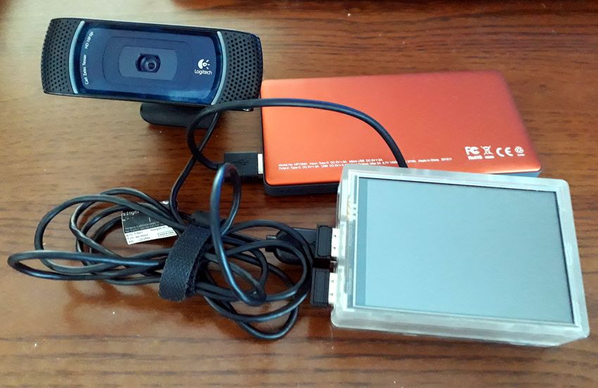
microcomputer was about 40$. Figure 4 presents a picture of the assembled microcomputer which was
used in this research.
Figure 4. The assembled microcomputer that was used in this research. It consists of a Raspberry Pi 3
model B+ in a semi-transparent case with a 3.5” LCD touchscreen, a Logitech Webcam C920 HD Pro, and a
powerbank (5 V, 3 A).
As was described in Section 2.2, the CelebA data set was divided into a training data set containing
180,000 ( 88% of CelebA) images and a validation data set that contained the rest of the data set ( 12% of
CelebA). As the validation data set contained over 22,000 images, leave-one-out cross validation was not
necessary. The same division was also used in [36].
In the case of the DNN proposed by Sandler et al. [36], I used two versions of it. The first version was
exactly the DNN version provided by the authors (https://github.com/Luca96/face-clustering), which
is named DNN 37 in Tables 3 and 4. This network annotates 37 attributes: the Attributes ’Attractive’,
’Pale_Skin’, and ’Blurry’ were skipped. The second version of this network had all 40 features and was
trained from scratch for the purposes of this paper, which is named DNN 40 in Tables 3 and 4. I set the
batch size to 32 and used 12 epochs. The whole training procedure, as described in detail in Section 2.2,
took less than 5 h.
The HOG–NN solution described in Section 2.3 used the same training and validation data set. It is
named NN 40 in Tables 3 and 4. Training of each of 40 networks took about 45 min.
Eigenfaces for the KNN classifier were generated from 50,000 images from the training dataset. I
took eigenvectors that explained approximately 99% of the variance (3128 eigenfeatures); this choice is
explained in Section 2.4. I tested 1-NN and 3-NN classifiers, which are named 1-NN and 3-NN in Tables
3 and 4. Their reference data was the full training data set consisting of 180,000 images. The validation
dataset was the same as that used for the previous classifiers.
All source code that was written for this paper is available online (https://github.com/
browarsoftware/FaceImagesAnnotation).Sensors 2020, 20, 2140 11 of 16
Table 3. Accuracy (expressed in percentage) of each classifier on each attribute.
Feature DNN 37 DNN 40 NN 40 3-NN 1-NN
X5_o_Clock_Shadow 93.32 93.34 90.78 88.05 85.5
Arched_Eyebrows 78.38 81.08 77.84 69.64 67.16
Attractive NA 78.46 75.43 66.77 64.15
Bags_Under_Eyes 80.81 83.44 82.32 77.6 74.21
Bald 98.84 98.39 97.76 97.66 96.86
Bangs 94.64 95 93.1 89.19 86.83
Big_Lips 69.31 70.3 69.29 65.46 62.72
Big_Nose 80.45 82.1 81.92 77.28 73.75
Black_Hair 76.63 72.35 82.15 71.77 68.45
Blond_Hair 87.85 88.13 93.26 89.02 87.28
Blurry NA 95.48 95.29 92.04 86.49
Brown_Hair 82 81.86 84.59 76.81 71.87
Bushy_Eyebrows 87.6 89.53 90.41 84.38 80.14
Chubby 95.25 95.15 94.84 94.35 92.95
Double_Chin 96.11 95.64 95.85 95.07 93.43
Eyeglasses 99.52 99.32 97.87 94.4 93.76
Goatee 96.97 96.69 96.1 95.12 93.3
Gray_Hair 97.62 96.44 97.32 96.65 95.41
Heavy_Makeup 67.8 80.38 85.53 75.64 72.48
High_Cheekbones 79.51 79.4 82.68 65.19 62.15
Male 92.39 95.22 94.58 83.11 80.71
Mouth_Slightly_Open 92.03 91.67 83.3 62.03 60.65
Mustache 96.59 96.65 96.5 96.05 94.6
Narrow_Eyes 86.88 86.09 86.66 83.75 80.02
No_Beard 95.06 94.09 92.31 85.9 83.55
Oval_Face 70.81 71.89 71.87 64.49 61.98
Pale_Skin NA 31.95 96.55 95.51 94.76
Pointy_Nose 74.75 71.88 73.81 67 63.6
Receding_Hairline 92.83 92.12 91.95 90.31 87.41
Rosy_Cheeks 92.83 92.83 93.7 91.62 88.95
Sideburns 97.41 97.34 96.37 95.31 93.28
Smiling 90.97 88.33 88.16 66.01 63.2
Straight_Hair 81.57 80.16 78.8 72.99 68.23
Wavy_Hair 77.28 78.75 73.29 67.34 64.88
Wearing_Earrings 84.58 87.71 81.45 77.15 73.68
Wearing_Hat 98.74 98.24 97.97 96.71 96.36
Wearing_Lipstick 67.86 90.27 90.84 79.21 75.23
Wearing_Necklace 86.31 86.28 85.92 81.89 78.24
Wearing_Necktie 96.7 95.44 94.75 92.95 91.05
Young 86.34 84.17 83.29 76.38 73.52
Averaged accuracy 87.15 86.59 88.20 82.19 79.57Sensors 2020, 20, 2140 12 of 16
Table 4. True positive rates (TPR) and true negative rates (TNR) of each classifier on each attribute
(expressed in percentage).
DNN 37 DNN 40 NN 40 3-NN 1-NN
Feature TPR TNR TPR TNR TPR TNR TPR TNR TPR TNR
X5_o_Clock_Shadow 38.97 99.35 45.54 98.65 58.81 94.39 22.77 95.43 31.76 91.58
Arched_Eyebrows 30.57 97.39 53.52 92.04 63.8 83.61 39.48 82.04 43.02 77.08
Attractive NA NA 66.05 90.66 89.59 60.82 68.51 64.96 65.85 62.4
Bags_Under_Eyes 71.52 83.18 31.67 96.59 39.98 93.25 18.98 92.74 27.03 86.4
Bald 74.23 99.38 40.9 99.63 17.66 99.45 6.59 99.59 17.07 98.55
Bangs 69.73 99.24 74.27 98.83 66.94 97.87 48.73 96.57 50.54 93.45
Big_Lips 8.98 98.63 31.54 89.14 20.57 92.98 19.94 87.59 27.86 79.67
Big_Nose 64.3 84.79 53.28 89.85 34.53 94.74 22.59 92.07 29.36 85.76
Black_Hair 23.88 96.29 10.88 95.27 49.93 94.06 35.61 85.13 40.15 78.91
Blond_Hair 9.14 99.95 11.88 99.85 62.06 98.22 47.56 95.61 50.72 93.09
Blurry NA NA 58.12 97.47 0.4 99.95 10.49 96.04 18.46 89.83
Brown_Hair 0 99.96 0.03 99.78 49.78 92.32 29.25 87.37 36.85 79.65
Bushy_Eyebrows 4.41 99.98 24.9 99.15 44.12 97.43 15.62 94.81 25.25 88.47
Chubby 14.18 99.79 18.62 99.43 25.56 98.66 9.16 99.04 16.65 97.16
Double_Chin 19.93 99.76 4.71 99.99 18.12 99.51 8.58 99.14 17.29 97.01
Eyeglasses 94.49 99.87 92.94 99.76 76.45 99.27 11.42 99.78 19.06 98.61
Goatee 45.9 99.42 71.91 97.88 33.29 99.06 10.36 99.11 17.27 96.88
Gray_Hair 57.08 98.95 68.87 97.35 38.32 99.22 21.36 99.07 30.34 97.51
Heavy_Makeup 20.61 99.92 53.54 98.64 92.95 80.28 67.74 81.24 64.38 78.22
High_Cheekbones 59.58 98.04 59.25 98.12 78.46 86.77 61.12 69.15 58.98 65.22
Male 99.21 88.1 96.09 94.68 90.54 97.04 72.84 89.38 71.71 86.21
Mouth_Slightly_Open 90.22 93.81 91.17 92.16 89.5 77.12 55.35 68.67 55.18 66.09
Mustache 19.69 99.68 27.2 99.44 22.6 99.32 3.04 99.61 10.12 97.83
Narrow_Eyes 18.83 98.76 9.84 99.41 21.93 97.74 5.18 97.2 13.47 91.42
No_Beard 98.7 73.78 95.33 86.85 97.04 64.52 95.77 27.92 91.7 35.7
Oval_Face 2 99.69 6.96 99.13 21.65 93.58 31.01 78.97 38.07 72.32
Pale_Skin NA NA 97.14 29.08 45.85 98.84 2 99.75 11.16 98.55
Pointy_Nose 21.32 96.13 2.09 99.8 35.01 89.63 32.96 80.88 38.97 73.64
Receding_Hairline 41.38 97.6 14.46 99.32 8.2 99.64 12.05 97.5 21.66 93.44
Rosy_Cheeks 0 100 0 100 24.64 99.13 13.3 97.78 22.25 94.2
Sideburns 52.92 99.57 67.71 98.78 37.97 99.21 10.7 99.43 17.91 96.96
Smiling 84.2 97.74 78.33 98.35 89.76 86.49 64.87 67.2 62.34 64.1
Straight_Hair 29.02 95.53 24.75 94.88 0 100 20.28 87.16 29.72 78.59
Wavy_Hair 40.46 98.36 48.3 96.19 50.34 86.66 44.61 80.57 46.31 75.69
Wearing_Earrings 27.73 99.38 52.34 96.92 24.93 96.57 20.81 92.22 29.32 85.54
Wearing_Hat 79.5 99.58 76.16 99.21 54.05 99.65 14.53 99.85 19.93 99.28
Wearing_Lipstick 38.49 99.92 84.81 96.23 88.66 93.34 78.7 79.79 73.8 76.88
Wearing_Necklace 1.05 99.95 1.6 99.83 0 100 15 92.86 23.48 87.21
Wearing_Necktie 72.27 98.55 39.81 99.63 42.67 98.66 19.2 98.49 28.44 95.76
Young 94.34 61.41 88.21 71.58 95.01 45.89 91.01 29.72 85.33 35.84
Averaged 43.75 95.98 46.87 94.74 47.54 92.12 31.98 87.04 36.97 83.52
4. Discussion
As can be seen in Table 3, the proposed method, which used the HOG face detector and the set of
40 NNs which performed annotation of each face attribute separately had the highest accuracy of all of the
validated classifiers. These results may, however, be misleading before examining the results in Table 4. As
can be seen in Table 4, no classifier has the highest TPR and TNR in all examined attributes. The 3-NN
and 1-NN classifiers had worse results than NN 40 most of the time; however, there were some attributes
that were classified better. For example, Wearing_Necklace and Wavy_Hair were not classified to separateSensors 2020, 20, 2140 13 of 16
classes by the NNs at all. These situations happen to be a limitation of the “classical” (not deep) NN
models. The averaged TPR and TNR strongly indicate that the classes were imbalanced, resulting in a
large difference in averaged TPR and TNR value for each attribute of the data set. It is not generally true
that TPR always had a smaller value than TNR (see, for example, the Young attribute); however, it caused
a disproportion in all classifiers, due to which TPR was over two times smaller than TNR. The reason
why TNR typically had a higher value than TPR in unbalanced classes is that, in the training data set,
there were much more negative than positive examples of particular attributes. We can easily conclude
that none of these methods, even the state-of-the-art [22] were capable of classifying the data set with
appropriate balance; that is, in a way that both TNR and TPR for each class had similarly high values (i.e.,
at the level of averaged accuracy of the certain classifier). The highest averaged TPR was obtained for NN
40 (47.54), the second highest was DNN 40 (46.87); the difference between those two was 0.67. The third
highest TNR was obtained for NN 37 (43.75); the difference between this one and the second was 3.12. In
case of TNR, the highest value was obtained for 30 DNN (95.98), the second highest was DNN 40 (94.74);
the difference between those two was 1.24. The third highest TNR was obtained for NN 40 (92.12); the
difference between this and the second was 2.62. Taking both averaged TPR and TNR into account, we can
conclude that DNN 40 might be slightly more effective than NN 40.
The real difference between these two models became visible while deploying them on a
microcomputer with very limited RAM. In the case of a microcontroller with 1 GB RAM (although
mobileNetV2 has been specifically tailored for mobile and resource constrained environments) both DNN
37 and DNN 40 failed at loading into the tested low power consumption device. On the other hand, it was
possible to successfully run NN 40 on the evaluated device, gradually loading and unloading each of the
networks after it performed annotation of a single attribute. It is also possible to perform online annotation
of human faces captured by the USB camera sensor connected to the device, as described in Section 3. The
source code for this application, together with the weights of the 40 NNs can be downloaded from the
same GitHub repository as the rest of the source code prepared for this paper.
The resource usage of the NN 40 method on PC and low power consumption microcomputer that
were presented in Section 3 was evaluated. I used the approach in which each NN is separately loaded
into memory, performs labelling, and then is unloaded from memory. It is done in order to not to exceed
the 1 GB memory of the microcomputer. The time required for HOG face detection (in resolution 640 ×
480), facial image aligning, loading single network model, and predicting face features were measured, as
well as the total time for processing one acquired frame (which includes all of the previous operations) and
labelling all 40 features. I also measured the RAM memory usage and CPU usage of the Python process.
The results averaged from 20 facial images acquired by USB camera are presented in Table 5.
PC HOG face detection was among most time-consuming operation in the image processing pipeline.
Face aligning, however, was very fast (4 milliseconds). The total time for face detection, aligning, and
labelling of all 40 features by loading and unloading the NN models individually was about 4.8 s. The
process occupied 1.1 GB of RAM and used 20.5% of CPU power. Annotation (predicting) of a single feature
took 27 milliseconds. When evaluating microcomputer processing, the times were significantly longer.
This situation can be easily explained when we compare memory usage: it was only 0.3 GB. This is because
the operating system performs memory swapping in order to not to exceed 1 GB of RAM, which is a
limit for the whole system. The swapping was performed on an SD memory card, so it was relatively
fast; however, RAM is important limitation in microcontrollers. The CPU usage was about 100%. This,
however, did not freeze the microcomputer; one can easily use other applications at the same time while
not expiring lags as the examined CPU has a multicore architecture. Annotation (prediction) time was
nearly 10 times slower than on PC (0.2 s per feature). Face aligning was nearly 15 times slower than on PC.
The annotation of all 40 features, individually loading and unloading models, took about 2 min. This was
quite a long time, compared to PC; however, we have to remember that the efficiency of the classifier on theSensors 2020, 20, 2140 14 of 16
microcomputer is the same as in PC and the price of PC used in this research was about 50 times higher (!)
than the microcomputer. Furthermore, one can easily linearly scale the performance of the NN 40 solution
by excluding classifiers that might be unnecessary for the certain task. Both on PC and microcontroller, the
proposed solution does not operate in real time (it was not higher than video frame acquisition time).
Table 5. Results of resource usage of the NN 40 method averaged from 20 measurements. Columns
represents (from left from right): time of HOG face detection, facial image aligning, loading single
network model, predicting face feature, total time for processing one acquired frame (including all previous
operations) and labelling of all 40 features, RAM memory usage of Python process, and CPU usage of
Python process.
Computer HOG [s] Aligning [s] Loading [s] Predicting [s] Total [s] RAM [GB] CPU [%]
PC 0.429 0.004 0.053 0.027 4.816 1.139 20.5
Raspberry 10.485 0.059 1.668 0.225 107.5 0.311 100
5. Conclusions
In this paper, I proposed an NN classifier designed for human face attribute annotation, which is
capable of running on relatively cheap, low power consumption systems. The proposed solution, consisting
of a HOG face detector and a set of neural networks, has comparable averaged accuracy and averaged
TPR and TNR to state-of-the-art DNNs; however, in contrast to the tested DNNs, it is possible to deploy
the proposed solution for limited RAM memory applications, such as microcomputers without additional
co-processors. Additional tests were carried out, proving that the implementation of the proposed method
can perform annotation of facial images acquired by an RGB camera, reusing virtually the same source
code and neural network weights, both on a high-end PC and a microcomputer. The results obtained can
be easily reproduced, as both the data set and source code are available online. The presented results are
especially important for researchers and engineers who develop autonomous systems based on low power
consumption, general-purpose microcomputers which need to perform autonomous classification tasks
without fast internet communication (i.e., without outsourcing image recognition to remote servers).
Funding: This research was funded by Pedagogical University of Krakow statutory research grant number
BS-203/M/2019.
Conflicts of Interest: The author declares no conflict of interest. The funder had no role in the design of the study;
in the collection, analyses, or interpretation of data; in the writing of the manuscript, or in the decision to publish
the results.
References
1. Zhong, Y.; Sullivan, J.; Li, H. Face attribute prediction using off-the-shelf CNN features. In Proceedings of the
2016 International Conference on Biometrics (ICB), Halmstad, Sweden, 13–16 June 2016; pp. 1–7.
2. Saez Trigueros, D.; Meng, L.; Hartnett, M. Face Recognition: From Traditional to Deep Learning Methods. J.
Theor. Appl. Inf. Technol. 2018, 97, 3332–3342.
3. Yang, S.; Nian, F.; Wang, Y.; Li, T.C. Real-time face attributes recognition via HPGC: Horizontal pyramid global
convolution. J. -Real-Time Image Process. 2019, 1–12. [CrossRef]
4. Dikle, S.; Shiurkar, U., Real Time Face Tracking and Recognition Using Efficient Face Descriptor and Features
Extraction Algorithms. In Computing in Engineering and Technology; Springer: Singapore, 2020; pp. 55–63.
doi:10.1007/978-981-32-9515-5_6. [CrossRef]
5. Rose, J.; Bourlai, T. Deep learning based estimation of facial attributes on challenging mobile phone face datasets.
In Proceedings of the 2019 IEEE/ACM International Conference on Advances in Social Networks Analysis and
Mining, Vancouver, BC, Canada, 27–30 August 2019; pp. 1120–1127. doi:10.1145/3341161.3343525. [CrossRef]Sensors 2020, 20, 2140 15 of 16
6. Csaba, B.; Tamás, H.; Horváth, A.; Oláh, A.; Reguly, I.Z. PPCU Sam: Open-source face recognition framework.
Procedia Comput. Sci. 2019, 159, 1947 – 1956. [CrossRef]
7. Chen, H.; Haoyu, C. Face Recognition Algorithm Based on VGG Network Model and SVM. J. Phys. Conf. Ser.
2019, 1229, 012015. doi:10.1088/1742-6596/1229/1/012015. [CrossRef]
8. Paul, L.; Suman, A. Face recognition using principal component analysis method. Int. J. Adv. Res. Comput. Eng.
Technol. 2012, 1, 135–139.
9. Wang, Y.; Gong, D.; Zhou, Z.; Ji, X.; Wang, H.; Li, Z.; Liu, W.; Zhang, T. Orthogonal Deep Features Decomposition
for Age-Invariant Face Recognition. In Computer Vision—ECCV 2018; Ferrari, V., Hebert, M., Sminchisescu, C.,
Weiss, Y., Eds.; Springer International Publishing: Cham, Switzerland, 2018; pp. 764–779.
10. Lucena, O.; Junior, A.; Moia, V.; Souza, R.; Valle, E.; Lotufo, R. Transfer Learning Using Convolutional Neural
Networks for Face Anti-spoofing. In Image Analysis and Recognition; Karray, F., Campilho, A., Cheriet, F., Eds.;
Springer International Publishing: Montreal, QC, Canada; Cham, Switzerland, 2017; pp. 27–34.
11. Aly, S.; Yanikoglu, B. Multi-Label Networks for Face Attributes Classification. In Proceedings of the 2018 IEEE
International Conference on Multimedia & Expo Workshops, San Diego, CA, USA, 23–27 July 2018; pp. 1–6.
doi:10.1109/ICMEW.2018.8551518. [CrossRef]
12. Fan, D.; Kim, H.; Kim, J.; Liu, Y.; Huang, Q. Multi-Task Learning Using Task Dependencies for Face Attributes
Prediction. Appl. Sci. 2019, 9, 2535. doi:10.3390/app9122535. [CrossRef]
13. Yilmaztürk, M.; Ulusoy, I.; Cicekli, N. Analysis of Face Recognition Algorithms for Online and Automatic
Annotation of Personal Videos. In Computer and Information Sciences; Springer: Dordrecht, The Netherlands, 2010;
Volume 62, pp. 231–236. doi:10.1007/978-90-481-9794-1_45. [CrossRef]
14. Conilione, P.; Wang, D. Automatic localization and annotation of facial features using machine learning
techniques. Soft Comput. 2011, 15, 1231–1245. doi:10.1007/s00500-010-0586-y. [CrossRef]
15. Nguyen, H.M.; Ly, N.Q.; Phung, T.T.T. Large-Scale Face Image Retrieval System at Attribute Level Based on
Facial Attribute Ontology and Deep Neuron Network. In Intelligent Information and Database Systems; Nguyen,
N.T., Hoang, D.H., Hong, T.P., Pham, H., Trawiński, B., Eds.; Springer International Publishing: Dong Hoi City,
Vietnam; Cham, Switzerland, 2018; pp. 539–549.
16. Wang, D.; Hoi, S.C.H.; He, Y. Mining Weakly Labeled Web Facial Images for Search-Based Face Annotation.
IEEE Trans. Knowl. Data Eng. 2011, 26, 166–179. [CrossRef]
17. Chang, J.R.; Juang, H.C.; Chen, Y.S.; Chang, C.M. Safe binary particle swam algorithm for an
enhanced unsupervised label refinement in automatic face annotation. Multimed. Tools Appl. 2016, 76.
doi:10.1007/s11042-016-4058-y. [CrossRef]
18. Firmino, A.; Baptista, C.; Figueirêdo, H.; Pereira, E.; Amorim, B. Automatic and semi-automatic
annotation of people in photography using shared events. Multimed. Tools Appl. 2018, 78, 13841–13875.
doi:10.1007/s11042-018-6715-9. [CrossRef]
19. Liu, Z.; Luo, P.; Wang, X.; Tang, X. Deep Learning Face Attributes in the Wild. In Proceedings of the 2015 IEEE
International Conference on Computer Vision (ICCV), Santiago, Chile, 7–13 December 2015; pp. 3730–3738.
doi:10.1109/ICCV.2015.425. [CrossRef]
20. Zhong, Y.; Sullivan, J.; Li, H. Leveraging mid-level deep representations for predicting face attributes in the wild.
In Proceedings of the 2016 IEEE International Conference on Image Processing (ICIP), Phoenix, AZ, USA, 25–28
September 2016; pp. 3239–3243. doi:10.1109/ICIP.2016.7532958. [CrossRef]
21. Torfason, R.; Agustsson, E.; Rothe, R.; Timofte, R. From Face Images and Attributes to Attributes; Springer: Cham,
Switzerland, 2016. doi:10.1007/978-3-319-54187-7_21. [CrossRef]
22. Anzalone, L.; Barra, P.; Barra, S.; Narducci, F.; Nappi, M. Transfer Learning for Facial Attributes Prediction and
Clustering. In Smart City and Informatization; Wang, G., El Saddik, A., Lai, X., Martinez Perez, G., Choo, K.K.R.,
Eds.; Springer: Singapore, 2019; pp. 105–117.
23. Becerra-Riera, F.; Morales-González, A.; Vazquez, H. A survey on facial soft biometrics for video surveillance
and forensic applications. Artif. Intell. Rev. 2019. doi:10.1007/s10462-019-09689-5. [CrossRef]
24. Ahmed, S.; Ali, S.; Ahmad, J.; Adnan, M.; Fraz, M. On the frontiers of pose invariant face recognition: A review.
Artif. Intell. Rev. 2019. doi:10.1007/s10462-019-09742-3. [CrossRef]Sensors 2020, 20, 2140 16 of 16
25. Zhang, J.; Zhan, R.; Sun, D.; Pan, G. Symmetry-Aware Face Completion with Generative Adversarial Networks.
In Computer Vision—ACCV 2018; Jawahar, C., Li, H., Mori, G., Schindler, K., Eds.; Springer International
Publishing: Cham, Switzerland, 2019; pp. 289–304.
26. Lu, Y.; Tai, Y.W.; Tang, C.K. Attribute-Guided Face Generation Using Conditional CycleGAN. In Computer
Vision—ECCV 2018; Ferrari, V., Hebert, M., Sminchisescu, C., Weiss, Y., Eds.; Springer International Publishing:
Cham, Switzerland, 2018; pp. 293–308.
27. Chhabra, S.; Singh, R.; Vatsa, M.; Gupta, G. Anonymizing k Facial Attributes via Adversarial Perturbations.
arXiv 2018, arXiv:1805.09380. doi:10.24963/ijcai.2018/91.
28. Flouty, E.; Zisimopoulos, O.; Stoyanov, D. FaceOff: Anonymizing Videos in the Operating Rooms. In OR 2.0
Context-Aware Operating Theaters, Computer Assisted Robotic Endoscopy, Clinical Image-Based Procedures, and Skin
Image Analysis; Stoyanov, D., Taylor, Z., Sarikaya, D., McLeod, J., González Ballester, M.A., Codella, N.C., Martel,
A., Maier-Hein, L., Malpani, A., Zenati, M.A., et al., Eds.; Springer International Publishing: Cham, Switzerland,
2018; pp. 30–38.
29. Ioffe, S.; Szegedy, C. Batch Normalization: Accelerating Deep Network Training by Reducing Internal Covariate
Shift. In Proceedings of the 32nd International Conference on Machine Learning, Lille, France, 7–9 July 2015.
30. Srivastava, N.; Hinton, G.; Krizhevsky, A.; Sutskever, I.; Salakhutdinov, R. Dropout: A Simple Way to Prevent
Neural Networks from Overfitting. J. Mach. Learn. Res. 2014, 15, 1929–1958.
31. Zeiler, M.D. ADADELTA: An Adaptive Learning Rate Method. arXiv 2012, arXiv:1212.5701.
32. Dalal, N.; Triggs, B. Histograms of oriented gradients for human detection. In Proceedings of the 2005 IEEE
Computer Society Conference on Computer Vision and Pattern Recognition (CVPR’05), San Diego, CA, USA,
20–25 June 2005; Volume 1, pp. 886–893, doi:10.1109/CVPR.2005.177. [CrossRef]
33. Kazemi, V.; Sullivan, J. One Millisecond Face Alignment with an Ensemble of Regression Trees. In Proceedings
of the IEEE Conference on Computer Vision and Pattern Recognition, Columbus, OH, USA, 23–28 June 2014,
doi:10.13140/2.1.1212.2243. [CrossRef]
34. Sagonas, C.; Antonakos, E.; Tzimiropoulos, G.; Zafeiriou, S.; Pantic, M. 300 Faces In-The-Wild Challenge:
database and results. Image Vis. Comput. 2016, 47, 3–18. doi:10.1016/j.imavis.2016.01.002. [CrossRef]
35. Kingma, D.P.; Ba, J. Adam: A Method for Stochastic Optimization. arXiv 2015, arXiv:1412.6980.
36. Sandler, M.; Howard, A.; Zhu, M.; Zhmoginov, A.; Chen, L. MobileNetV2: Inverted Residuals and Linear
Bottlenecks. In Proceedings of the 2018 IEEE/CVF Conference on Computer Vision and Pattern Recognition,
Salt Lake City, UT, USA, 18–23 June 2018; pp. 4510–4520. doi:10.1109/CVPR.2018.00474. [CrossRef]
c 2020 by the authors. Licensee MDPI, Basel, Switzerland. This article is an open access
article distributed under the terms and conditions of the Creative Commons Attribution (CC
BY) license (http://creativecommons.org/licenses/by/4.0/).You can also read